![]()
Expanding on Data Type Concepts
You have learned how to retrieve data from SQL Server tables in a number of ways: through simple queries, through joins, with functions, and more. You have learned to manipulate data, write scripts, and create database objects. Essentially, you have learned the T-SQL basics. Not only have you learned the mechanics of T-SQL, but you have also learned to think about the best way to solve a problem, not just the easy way.
This chapter introduces some of the more interesting and complex data types available in SQL Server. You will learn about sparse columns, built-in complex types (HIERARCHYID, GEOMETRY, and GEOGRAPHY), enhanced date and time data types, large-value data types (MAX), and FILESTREAM data. Some of these, such as the complex data types, are nothing like the traditional data types you have been using throughout this book. They are based on the CLR (Common Language Runtime). New data types similar to these built-in complex types can be created with a .NET language. You will not learn to create new data types from this book, but you will learn how to use the built-in CLR types.
Chapters 1 through 14 covered the important skills you need to become a proficient T-SQL developer. Chapter 15 covered working with XML in SQL Server. Because this chapter covers “bonus material,” it doesn’t contain exercises. I encourage you to practice working with any of the new data types that interest you or that you think will be beneficial in your job.
Large-Value String Data Types (MAX)
Older versions of SQL Server used NTEXT and TEXT data types to represent large values. Microsoft has deprecated those types, which means that in some future release of SQL Server, NTEXT and TEXT will no longer work. For now, however, the deprecated data types still work in SQL Server 2014. Going forward, you should replace these data types with VARCHAR(MAX) and NVARCHAR(MAX).
The TEXT and NTEXT data types have many limitations. For example, you can’t declare a variable of type TEXT or NTEXT, use them with most functions, or use them within most search criteria. The MAX data types represent the benefits of both the regular string data types and the TEXT and NTEXT data types when storing large strings. They allow you to store large amounts of data and offer the same functionality of the traditional data types.
When creating string data types, you supply a number of characters. Instead of supplying a number, use the word MAX when the data is going to surpass the maximum normally allowed. Table 16-1 lists the differences between the string value data types.
Table 16-1. The String Data Types

![]() Note One difference between CHAR/VARCHAR and NCHAR/NVARCHAR when specifying a literal string is that the NCHAR/NVARCHAR types should be preceded by the letter N. This tells the query processor to interpret the string as Unicode. If you don’t precede the literal string with the letter N, the code will usually still work.
Note One difference between CHAR/VARCHAR and NCHAR/NVARCHAR when specifying a literal string is that the NCHAR/NVARCHAR types should be preceded by the letter N. This tells the query processor to interpret the string as Unicode. If you don’t precede the literal string with the letter N, the code will usually still work.
You work with the MAX string data types just like you do with the traditional types for the most part. Type in and execute Listing 16-1 to learn how to work with the MAX types.
Listing 16-1. Using VARCHAR(MAX)
--1
CREATE TABLE #maxExample (maxCol VARCHAR(MAX),
    line INT NOT NULL IDENTITY PRIMARY KEY);
GO

--2
INSERT INTO #maxExample(maxCol)
VALUES ('This is a varchar(max)'),

--3
INSERT INTO #maxExample(maxCol)
VALUES (REPLICATE('aaaaaaaaaa',9000));

--4
INSERT INTO #maxExample(maxCol)
VALUES (REPLICATE(CONVERT(VARCHAR(MAX),'bbbbbbbbbb'),9000));

--5
SELECT LEFT(MaxCol,10) AS Left10,LEN(MaxCol) AS varLen
FROM #maxExample;

GO
DROP TABLE #maxExample;
Figure 16-1 shows the results of running this code. Statement 1 creates a temp table, #maxExample, with a VARCHAR(MAX) column. Statement 2 inserts a row into the table with a short string. Statement 3 inserts a row using the REPLICATE function to create a very large string. If you look at the results, the row inserted by statement 3 contains only 8,000 characters. Statement 4 also inserts a row using the REPLICATE function. This time the statement explicitly converts the string to be replicated to a VARCHAR(MAX). That is because, without explicitly converting it, the string is just a VARCHAR. The REPLICATE function, like most string functions, returns the same data types as supplied to it. To return a VARCHAR(MAX), the function must receive a VARCHAR(MAX). Statement 5 uses the LEFT function to return the first ten characters of the value stored in the maxCol column, demonstrating that you can use string functions with VARCHAR(MAX). Attempting to use LEFT on a TEXT column will just produce an error. It uses the LEN function to see how many characters the column stores in each row. Only 8,000 characters of the row inserted in statement 3 made it to the table because the value wasn’t explicitly converted to VARCHAR(MAX) before the REPLICATE function was applied.

Figure 16-1. The results of using the VARCHAR(MAX) data type
If you get a chance to design a database, you may be tempted to make all your string value columns into MAX columns. Microsoft recommends that you use the MAX data types only when it is likely that you will exceed the 8,000- or 4,000-character limits. To be most efficient, size your columns to the expected data.
You probably have less experience with the data types that store binary data. You can use BINARY, VARBINARY, and IMAGE to store binary data including files such as images, movies, and Word documents. The BINARY and VARBINARY data types can hold up to 8,000 bytes. The IMAGE data type, which is deprecated like the TEXT and NTEXT types, holds data that exceeds 8,000 bytes, up to 2GB. In SQL Server versions 2005 and greater, always use the VARBINARY(MAX) data type, which can store up to 2GB of binary data, instead of IMAGE.
To store data into a VARBINARY(MAX) column, or any of the binary data columns, you can use the CONVERT or CAST function to change string data into binary data. If you have data that is already in hexadecimal format, you can add 0x in front of it instead of casting. Using a program written in a .NET language or any language type that supports working with SQL Server, you can save actual files into VARBINARY(MAX) columns. In this simple demonstration, you will add data by converting string data. Type in and execute Listing 16-2 to learn more.
Listing 16-2. Using VARBINARY(MAX) Data
--1
CREATE TABLE #BinaryTest (DataDescription VARCHAR(50),
    BinaryData VARBINARY(MAX));

--2
INSERT INTO #BinaryTest (DataDescription,BinaryData)
VALUES ('Test 1', CONVERT(VARBINARY(MAX),'this is the test 1 row')),
    ('Test 2', CONVERT(VARBINARY(MAX),'this is the test 2 row'));

--3
SELECT DataDescription, BinaryData, CONVERT(VARCHAR(MAX), BinaryData)
FROM #BinaryTest;

--4
DROP TABLE #BinaryTest;
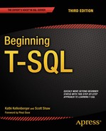
Figure 16-2 shows the results of running this code. Statement 1 creates the #BinaryTest table containing the BinaryData column of type VARBINARY(MAX). corStatement 2 inserts two rows. To insert data into the BinaryData column, it must be converted into a binary type. Query 3 displays the data. To read the data, the statement converts it back into a string data type.
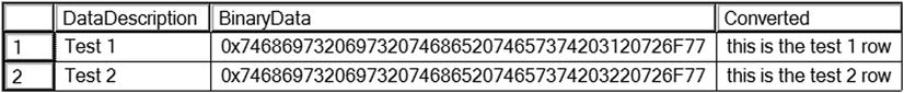
Figure 16-2. The results of using a VARBINARY(MAX) column
Often database applications involving files, such as images or Word documents, store just the path to the file in the database and store the actual file on a share in the network. This can be more efficient than storing large files within the database because the file system works more efficiently than SQL Server with streaming file data. This solution also poses some problems. Because the files live outside the database, you have to make sure they are secure. You can’t automatically apply the security as set up in the database to the files. Another issue is backups. When you back up a database, how do you make sure that the backups of the documents in the file shares are done at the same time so the data is consistent in case of a restore?
The FILESTREAM object solves these issues by storing the files on the file system but making the files become part of the database. This is the recommended solution if the files are over 1MB in size. To add and manipulate files, you must use T-SQL commands. In addition, an API is available for modifying the files, although this solution is rather cumbersome.
To set up a FILESTREAM object, add the word FILESTREAM to the VARBINARY(MAX) column when creating the table. The SQL Server instance must be configured to allow FILESTREAM data, and the database must have a filegroup defined for FILESTREAM data. To configure the SQL Server instance to allow FILESTREAM data, follow these instructions:
- Launch the SQL Server Configuration Manager utility as shown in Figure 16-3.
Figure 16-3. The SQL Server Configuration Manager
- Select SQL Server Services and locate the SQL Server instance as shown in Figure 16-4.

Figure 16-4. The SQL Server Instance
- Double-click the Instance and select the FILESTREAM tab as shown in Figure 16-5. Make sure that all options are enabled. By checking Enable FILESTREAM for file I/O access you will turn on the FileTable functionality (discussed in the next section). Allowing remote access lets users from other systems access the files.
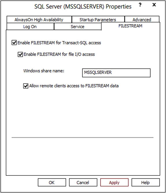
Figure 16-5. Enable Filestream
- Click OK. If changes were made, restart the SQL Server.
SQL Server databases have a minimum of two files: the data file and the log file. To use the Filestream functionality in a database, you will add a special filegroup and add a file to the filegroup. To add Filestream to AdventureWorks, follow these instructions:
- Right-click the AdventureWorks database and select Properties.
- Select Filegroups.
- In the FILESTREAM section, click Add Filegroup. A new row will appear in the FILESTREAM section.
- Type FileStream in the name as shown in Figure 16-6.
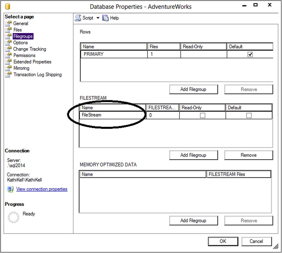
Figure 16-6. Adding a filegroup
- Select the Files page.
- Click Add, and then type in AWFS in the Logical Name property in the new row.
- Under File Type, select FILESTREAM Data as shown in Figure 16-7.

Figure 16-7. Add the File Type property
- Scroll to the right and locate the Path property of the AWFS logical file. Click the ellipsis button to set the location of the new file. Make a note of the Path property so you will have it available later in the chapter.
- Click OK. Now the AdventureWorks database is set up for FILESTREAM data.
To create a FILESTREAM column, you just add the word FILESTREAM to the VARBINARY(MAX) column definition when it is created. Listing 16-3 creates and populates a FILESTREAM type column.
Listing 16-3. Working with a FILESTREAM Column
--1
IF OBJECT_ID('dbo.NotepadFiles') IS NOT NULL BEGIN
    DROP TABLE dbo.NotepadFiles;
END;

--2
CREATE table dbo.NotepadFiles(Name VARCHAR(25),
    FileData VARBINARY(MAX) FILESTREAM,
    RowID UNIQUEIDENTIFIER ROWGUIDCOL
        NOT NULL UNIQUE DEFAULT NEWSEQUENTIALID());

--3
INSERT INTO dbo.NotepadFiles(Name,FileData)
VALUES ('test1', CONVERT(VARBINARY(MAX),'This is a test')),
    ('test2', CONVERT(VARBINARY(MAX),'This is the second test'));

--4
SELECT Name,FileData,CONVERT(VARCHAR(MAX),FileData) TheData, RowID
FROM dbo.NotepadFiles;
Figure 16-8 shows the results of running this code. Code section 1 drops the NotepadFiles table in case it already exists. Statement 2 creates the NotepadFiles table. The Name column contains a value to help identify the row. The FileData column is the FILESTREAM column. To create the FILESTREAM column, specify the FILESTREAM keyword when creating a VARBINARY(MAX) column. The RowID column has a special setting ROWGUIDCOL, which specifies that the column is automatically updated with a unique global identifier. The NEWSEQUENTIALID function populates the RowID column. This function creates a unique value for each row, which is required when using FILESTREAM data.

Figure 16-8. The results of populating a FILESTREAM column
Statement 3 inserts two rows into the table. The data to be inserted into the FileData column must be of type VARBINARY(MAX) so the statement converts it. Statement 4 shows the results. The FileData column displays the binary data. By converting it to VARCHAR(MAX), you can read the data. Navigate to the appropriate folder on your system through the path you saved when setting up the FileStream filegroup. You should see an AWFS folder. You will get a warning saying you don’t have permission to access the folder. You can click Continue to view the contents.
Inside the AWFS folder is a folder with a unique identifier name; this folder corresponds to the dbo.NotepadFiles table you created in the last demo because it has a FILESTREAM column. Figure 16-9 shows the AWFS folder on my system.
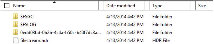
Figure 16-9. The ASFS folder
If you navigate further down in the unique identifier named folder to the actual files, you will see two files that can be opened in Notepad. The text inside those files will match the data demonstrated in Listing 16-3. When working with a production database, the user would have an application that opens the file through calls to SQL Server with the appropriate program, not by navigating to the actual file. In a non-laboratory environment, do not open the files directly.
When you delete a row from the NotepadFiles table, the corresponding file on disk will also disappear. If you drop the table, the entire folder will disappear. Run this code, and then check the Documents folder once again:
DROP TABLE NotepadFiles;
CHECKPOINT;
The database engine doesn’t delete the folder until the database commits all transactions to disk, called a checkpoint. By running the CHECKPOINT command, you force the checkpoint.
Building on the FILESTREAM technology, SQL Server 2012 introduced an exciting new feature called FileTables. FileTables allow you to store files like movies, documents, or music in an SQL Server table but still allows access to them through Windows Explorer or through another application. The fact that these files are stored in the file system but controlled by SQL Server is transparent to the user but, because they are part of the database, you get many of the benefits of a relational database, such as the ability to query file properties using T-SQL and security.
Because the data stored in a FileTable is not your normal data, you will need to first tell SQL Server to treat the data differently. You do this by telling SQL Server the data is non-transactional. A FileTable requires a directory name so you create one in your ALTER DATABASE statement. I chose the name FileTableDocuments. After running the ALTER DATABASE script, you are now able to create a FileTable. In my example, I created a FileTable name MyDocuments that points to a directory called Misc Documents. As you’ll see later, the Misc Documents folder will be created under the FileTableDocuments folder. Listing 16-4 shows both queries.
Listing 16-4. Creating a FileTable
USE MASTER;
GO
ALTER DATABASE AdventureWorks
    SET FILESTREAM ( NON_TRANSACTED_ACCESS = FULL, DIRECTORY_NAME = 'FileTableDocuments'),
GO

USE AdventureWorks;
GO

CREATE TABLE MyDocuments AS FileTable
    WITH (
          FileTable_Directory = 'Misc Documents',
          FileTable_Collate_Filename = SQL_Latin1_General_CP1_CI_AS
         );
GO
If the command doesn’t work in a couple of seconds, you may need to close all connections to the database first. One thing to note is when creating the FileTable, I needed to specify the collation. In some cases, the AdventureWorks database download is case sensitive and FileTables can’t be created with a case-sensitive collation. The collation I specified in the CREATE TABLE statement is case insensitive. Also note I did not include any column names in my CREATE TABLE statement. This is because a FileTable has a default set of columns that can’t be altered. These columns refer to key metadata information on the file stored in the table.
Now that you have the FileTable created, you get to the fun part. There are two ways to get to the directory, or contents, of the table. The first way is through SQL Server Management Studio. If you navigate to the Tables folder under the AdventureWorks database, you will notice an additional folder called FileTables. If you expand the folder, you will see the table created in Listing 16-4. Figure 16-10 shows where the FileTable object can be found in SQL Server Management Studio.
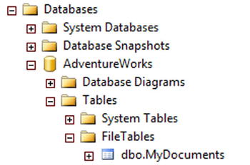
Figure 16-10. FileTable in SQL Server Management Studio
Right-click the file table and select Explore FileTable Directory. Once the folder opens, notice the full path to the directory in the address bar. In my case, the full path is \Kathikellsql2014FileTableDocumentsMisc Documents. This leads to the second method of getting to the folder. You can access this folder by typing the UNC path in the run bar under your Windows Start menu. This is also the path you can share with other users who need to place files in the directory.
Right now the FileTable is empty, as is the folder. You can confirm this by executing a SELECT statement against the table and noticing that no rows are returned. So let’s put a file in the folder. You can either create a new file like a .txt file or you can copy an existing file into the directory. In my example, I will right-click the empty directory and create a blank text file called FileTableTest.txt. After the file is created, run a SELECT statement against the table. Figure 16-11 shows the partial results of my SELECT statement.
![]()
Figure 16-11. Viewing a document in a FileTable
You now have a text document stored in a database table, but it can be viewed through Windows Explorer as if it were stored on a file system. If you delete the file from the folder, the row will be removed from the table. If you delete the row from the table, the file will be removed from the folder. This means you get many of the benefits of a relational database including all the backup, recovery, and security options SQL Server offers but with the simplicity of Windows file navigation.
You can also use T-SQL statements to create and delete files by inserting rows into the MyDocuments table. Type in and run the following statement and then take a look at the share again. You can open the file with Wordpad to see the contents.
INSERT INTO [dbo].[MyDocuments]
           ([file_stream]
           ,[name])
     VALUES
           (cast('hello' as varbinary(max)),'MyNewFile.txt'),
GO
Enhanced Date and Time
Previous versions of SQL Server have the DATETIME and SMALLDATETIME data types for working with temporal data. One big complaint by developers has been that there wasn’t an easy way to store just dates or just time. SQL Server contains several temporal data types. You have a choice of using the DATE and TIME data types as well as the DATETIME2 and DATETIMEOFFSET data types.
Using DATE, TIME, and DATETIME2
You can store just a date or time value by using the new DATE and TIME data types. The traditional DATETIME and SMALLDATETIME data types default to 12 a.m. when you don’t specify the time. You can also specify a precision, from zero to seven decimal places, when using the TIME and DATETIME2 data types. Type in and execute Listing 16-5 to learn how to use the new types.
Listing 16-5. Using DATE and TIME
USE tempdb;

--1
IF OBJECT_ID('dbo.DateDemo') IS NOT NULL BEGIN
    DROP TABLE dbo.DateDemo;
END;


--2
CREATE TABLE dbo.DateDemo(JustTheDate DATE, JustTheTime TIME(1),
    NewDateTime2 DATETIME2(3), UTCDate DATETIME2);


--3
INSERT INTO dbo.DateDemo (JustTheDate, JustTheTime, NewDateTime2,
    UTCDate)
VALUES (SYSDATETIME(), SYSDATETIME(), SYSDATETIME(), SYSUTCDATETIME());

--4
SELECT JustTheDate, JustTheTime, NewDateTime2, UTCDate
FROM dbo.DateDemo;
Figure 16-12 shows the results of running this code. Code section 1 drops the dbo.DateDemo table if it already exists. Statement 2 creates the dbo.DateDemo table with a DATE, a TIME, and two DATETIME2 columns. Notice that the TIME and DATETIME2 columns have the precision specified. The default is seven places if a precision is not specified. Statement 3 inserts a row into the table using the SYSDATETIME function. This function works like the GETDATE function except that it has greater precision than GETDATE. The statement populates the UTCDate column with the SYSUTCDATETIME function, which provides the Coordinated Universal Time (UTC). Statement 4 shows the results. The JustTheDate value shows that even though the SYSDATETIME function populated it, it stored only the date. The JustTheTime values stored only the time with one decimal place past the seconds. The NewDateTime2 column stored both the date and time with three decimal places. The UTCDate column stored the UTC date along with seven decimal places. Because the computer running this demo is in Central time, the time is five hours different.

Figure 16-12. The results of using the new date and time data types
Most business applications won’t require the default precision of seven places found with the TIME and DATETIME2 types. Be sure to specify the required precision when creating tables with columns of these types to save space in your database.
The new DATETIMEOFFSET data type contains, in addition to the date and time, a time zone offset for working with dates and times in different time zones. This is the difference between the UTC date/time and the stored date. Along with the new data type, several new functions for working with DATETIMEOFFSET are available. Type in and execute Listing 16-6 to learn how to work with this new data type.
Listing 16-6. Using the DATETIMEOFFSET Data Type
USE tempdb;

--1
IF OBJECT_ID('dbo.OffsetDemo') IS NOT NULL BEGIN
    DROP TABLE dbo.OffsetDemo;
END;

--2
CREATE TABLE dbo.OffsetDemo(Date1 DATETIMEOFFSET);


--3
INSERT INTO dbo.OffsetDemo(Date1)
VALUES (SYSDATETIMEOFFSET()),
    (SWITCHOFFSET(SYSDATETIMEOFFSET(),'+00:00')),
    (TODATETIMEOFFSET(SYSDATETIME(),'+05:00'));


--4
SELECT Date1
FROM dbo.OffsetDemo;
Figure 16-13 shows the results of running this code. Code section 1 drops the dbo.OffsetDemo table if it exists. Statement 2 creates the table with a DATETIMEOFFSET column, Date1. Statement 3 inserts three rows into the table using the new functions for working with the new data types. The SYSDATETIMEOFFSET function returns the date and time on the server along with the time zone offset. The computer I am using is five hours behind UTC, so the value –05:00 appears after the current date and time. Using the SWITCHOFFSET function, you can switch a DATETIMEOFFSET value to another time zone. Notice that by switching to +00:00, the UTC time, the date, and time values adjust. By using the TODATETIMEOFFSET function, you can add a time zone to a regular date and time.
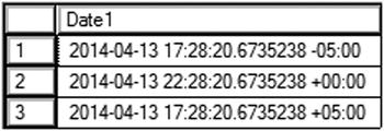
Figure 16-13. The results of using DATETIMEOFFSET
The DATETIMEOFFSET type and functions may be useful to you if you work with data in different time zones. When time changes go into effect, such as Daylight Saving Time, the offsets don’t adjust. Keep that in mind if you choose to work with DATETIMEOFFSET.
HIERARCHYID
The HIERARCHYID data type is used to represent hierarchical relationships in data, for example, family trees, which means that it can contain multiple properties instead of just one value. The HIERARCHYID column also has methods, which means that columns and variables of this type can “do something” and not just contain a value. The HIERARCHYID data type originally shipped with SQL Server 2008, and you can use it even if you don’t want to create any custom types.
You learned about joining a table to itself in the “Self-Joins” section in Chapter 5. In older versions of AdventureWorks, the ManagerID column points back to the EmployeeID column in the HumanResources.Employee table. To follow the organizational chart from this table, you must recursively follow the chain of command from the CEO down each manager-employee path to the lowest employee, which is pretty difficult to do with T-SQL. Chapter 11 covered how to do this in the “Writing a Recursive Query” section. The 2012 AdventureWorks database replaces the self-join with OrganizationalNode, a HIERARCHYID column, which is much easier to query.
If you just write a query to view the OrganizationalNode in the HumanResources.Employee table, you will see binary data. That is because CLR data types are stored as binary values. To view the data in readable form, you must use the ToString method of the type. The OrganizationalLevel column in the table is a computed column based on OrganizationalNode using the GetLevel method. Type in and execute Listing 16-7 to view the data.
Listing 16-7. Viewing the OrganizationalNode
USE AdventureWorks;
GO
SELECT BusinessEntityID,
    SPACE((OrganizationLevel) * 3) + JobTitle AS Title,
    OrganizationNode, OrganizationLevel,
    OrganizationNode.ToString() AS Readable
FROM HumanResources.Employee
ORDER BY Readable;
Figure 16-14 shows the partial results of running this code. As mentioned, the OrganizationalNode data is meaningless unless you use the ToString method as in the Readable column. By using the SPACE function to indent the JobTitle column from the table to produce the Title column in the results and by sorting on the Readable column, you can see the relation between the job titles in the data.

Figure 16-14. The partial results of querying the HumanResources.Employee table
The very first node in the hierarchy is the CEO (chief executive officer) of the company, represented as a slash (/) in the Readable column. The level for the CEO is 0, which you can see in the computed column OrganizationLevel. Several employees have an OrganizationLevel of 1; these employees report directly to the CEO. If you scroll down through all the results, you will see that these have a value, 1 through 6, in between two slashes. The vice president of engineering is the first node in level 1. The marketing manager is the second node in level 1. Each of these employees has other employees reporting to them. Those employees have a level of 2. For example, the engineering manager reports to the vice president of engineering and has a Readable value of /1/1/. Four employees report to the engineering manager. These employees all have Readable values that begin with /1/1/ along with an additional value, 1 through 4.
As you can see from the previous example, querying hierarchical data using HIERARCHYID is not difficult. Maintaining the data, however, is much more challenging. To add a new value or update existing values, you must use the built-in methods of the data type. If you have worked with nodes and pointers in other programming languages, you will find this to be very similar. To learn how to insert nodes using these methods to create hierarchical data, download or type in and execute the code in Listing 16-8.
Listing 16-8. Creating a Hierarchy with HIERARCHYID
Use tempdb;


--1
IF OBJECT_ID('SportsOrg') IS NOT NULL BEGIN
     DROP TABLE SportsOrg;
END;


--2
CREATE TABLE SportsOrg
    (DivNode HIERARCHYID NOT NULL PRIMARY KEY CLUSTERED,
    DivLevel AS DivNode.GetLevel(), --Calculated column
    DivisionID INT NOT NULL,
    Name VARCHAR(30) NOT NULL);


--3
INSERT INTO SportsOrg(DivNode,DivisionID,Name)
VALUES(HIERARCHYID::GetRoot(),1,'State'),


--4
DECLARE @ParentNode HIERARCHYID, @LastChildNode HIERARCHYID;

--5
SELECT @ParentNode = DivNode
FROM SportsOrg
WHERE DivisionID = 1;

--6
SELECT @LastChildNode = max(DivNode)
FROM SportsOrg
WHERE DivNode.GetAncestor(1) = @ParentNode;

--7
INSERT INTO SportsOrg(DivNode,DivisionID,Name)
VALUES (@ParentNode.GetDescendant(@LastChildNode,NULL),
2,'Madison County'),

--8
SELECT DivisionID,DivLevel,DivNode.ToString() AS Node,Name
FROM SportsOrg;
Figure 16-15 shows the results of running this code. You might be surprised how much code was required just to insert two rows! Code section 1 drops the SportsOrg table if it already exists. Statement 2 creates the SportsOrg table with the DivisionID and Name columns to identify each division or team. The DivNode column is a HIERARCHYID column, and the DivLevel is a computed column. Statement 3 inserts the first row, the root, into the table. Take a close look at the INSERT statement. Instead of inserting a value into DivNode, the statement uses the name of the data type along with the GetRoot method. Of course, because DivLevel is a computed column, you don’t insert anything into it.

Figure 16-15. The results of creating a hierarchy
To insert the second and subsequent nodes, you have to use the GetDescendant method of the parent node. You also have to determine the last child of the parent. Statement 4 declares two variables needed to accomplish this. Statement 5 saves the parent into a variable. Statement 6 saves the last child of the parent into a variable. In this case, there are no children just yet. Statement 7 inserts the row using the GetDescendant method. If the second argument is NULL, the method returns a new child that is greater than the child node in the first argument. Finally, query 8 displays the data.
Using Stored Procedures to Manage Hierarchical Data
Working with HIERARCHYID can be pretty complicated, as shown in the previous section. If you decide to use this data type in your applications, I recommend that you create stored procedures to encapsulate the logic and make coding your application much easier. Listing 16-9 contains a stored procedure to add new rows to the table. There is a lot of code to type so you may want to download the code from the book’s web site (www.apress.com) instead of typing it in. Execute the code to learn more.
Listing 16-9. Using a Stored Procedure to Insert New Nodes
USE tempdb;
GO

--1
IF OBJECT_ID('dbo.usp_AddDivision') IS NOT NULL BEGIN
    DROP PROC dbo.usp_AddDivision;
END;
IF OBJECT_ID('dbo.SportsOrg') IS NOT NULL BEGIN
    DROP TABLE dbo.SportsOrg;
END;
GO

--2
CREATE TABLE SportsOrg
    (DivNode HierarchyID NOT NULL PRIMARY KEY CLUSTERED,
    DivLevel AS DivNode.GetLevel(), --Calculated column
    DivisionID INT NOT NULL,
    Name VARCHAR(30) NOT NULL);
GO

--3
INSERT INTO SportsOrg(DivNode,DivisionID,Name)
VALUES(HIERARCHYID::GetRoot(),1,'State'),
GO

--4
CREATE PROC usp_AddDivision @DivisionID INT,
    @Name VARCHAR(50),@ParentID INT AS
    SET TRANSACTION ISOLATION LEVEL SERIALIZABLE;

    DECLARE @ParentNode HierarchyID, @LastChildNode HierarchyID;

    --Grab the parent node
    SELECT @ParentNode = DivNode
    FROM SportsOrg
    WHERE DivisionID = @ParentID;

    BEGIN TRANSACTION
        --Find the last node added to the parent
        SELECT @LastChildNode = max(DivNode)
        FROM SportsOrg
        WHERE DivNode.GetAncestor(1) = @ParentNode;
        --Insert the new node using the GetDescendant function
        INSERT INTO SportsOrg(DivNode,DivisionID,Name)
        VALUES (@ParentNode.GetDescendant(@LastChildNode,NULL),
            @DivisionID,@Name);
    COMMIT TRANSACTION;
GO

--5
EXEC usp_AddDivision 2,'Madison County',1;
EXEC usp_AddDivision 3,'Macoupin County',1;
EXEC usp_AddDivision 4,'Green County',1;
EXEC usp_AddDivision 5,'Edwardsville',2;
EXEC usp_AddDivision 6,'Granite City',2;
EXEC usp_AddDivision 7,'Softball',5;
EXEC usp_AddDivision 8,'Baseball',5;
EXEC usp_AddDivision 9,'Basketball',5;
EXEC usp_AddDivision 10,'Softball',6;
EXEC usp_AddDivision 11,'Baseball',6;
EXEC usp_AddDivision 12,'Basketball',6;
EXEC usp_AddDivision 13,'Ages 10 - 12',7;
EXEC usp_AddDivision 14,'Ages 13 - 17',7;
EXEC usp_AddDivision 15,'Adult',7;
EXEC usp_AddDivision 16,'Preschool',8;
EXEC usp_AddDivision 17,'Grade School League',8;
EXEC usp_AddDivision 18,'High School League',8;

--6
SELECT DivNode.ToString() AS Node,
    DivisionID, SPACE(DivLevel * 3) + Name AS Name
FROM SportsOrg
ORDER BY DivNode;
Figure 16-16 shows the results of running this code. Code section 1 drops the stored procedure and table if they already exist. Statement 2 creates the table, and statement 3 inserts the root as in the previous section. Code section 4 creates the stored procedure to insert new nodes. The stored procedure requires the new DivisionID and Name values along with the DivisionID of the parent node. Inside the stored process, an explicit transaction contains the code to grab the last child node and perform the insert. If this were part of an actual multiuser application, it would be very important to make sure that two users didn’t accidentally insert values into the same node position. By using an explicit transaction with serializable isolation, you avoid that problem. Code section 5 calls the stored procedure to insert each node. Finally, query 6 retrieves the data from the SportsOrg table. The query uses the same technique from the previous section utilizing the SPACES function to format the Name column results.

Figure 16-16. The results of using a stored procedure to insert new rows
Deleting a node is easy; you just delete the row. Unfortunately, there is nothing built into the HIERARCHYID data type to ensure that the children of the deleted nodes are also deleted or moved to a new parent. You will end up with orphaned nodes if the deleted node was a parent node. You can also move nodes, but you must make sure that you move the children of the moved parent nodes as well. If you decide to include the HIERARCHYID in your applications, be sure to learn about this topic in depth before you design your application. See Books Online for more information about how to work with HIERARCHYID.
In the previous section, you learned about the CLR data type HIERARCHYID. SQL Server has two other CLR data types, GEOMETRY and GEOGRAPHY, also known as the spatial data types. The GEOMETRY data type might be used for a warehouse application to store the location of each product in the warehouse. The GEOGRAPHY data type can be used to store data that can be used in mapping software. You may wonder why two types that both store locations exist. The GEOMETRY data type follows a “flat Earth” model, with basically X, Y, and Z coordinates. The GEOGRAPHY data type represents the “round Earth” model, storing longitude and latitude. These data types implement international standards for spatial data.
By using the GEOMETRY type, you can store points, lines, and polygons. You can calculate the difference between two shapes, determine whether they intersect, and much more. Just like HIERARCHYID, the database engine stores the data as a binary value. GEOMETRY also has many built-in methods for working with the data. Type in and execute Listing 16-10 to learn how to use the GEOMETRY data type with some simple examples.
Listing 16-10. Using the GEOMETRY Data Type
USE tempdb;
GO

--1
IF OBJECT_ID('dbo.GeometryData') IS NOT NULL BEGIN
    DROP TABLE dbo.GeometryData;
END;

--2
CREATE TABLE dbo.GeometryData (
    Point1 GEOMETRY, Point2 GEOMETRY,
    Line1 GEOMETRY, Line2 GEOMETRY,
    Polygon1 GEOMETRY, Polygon2 GEOMETRY);

--3
INSERT INTO dbo.GeometryData (Point1, Point2, Line1, Line2, Polygon1, Polygon2)
VALUES (
    GEOMETRY::Parse('Point(1 4)'),
    GEOMETRY::Parse('Point(2 5)'),
    GEOMETRY::Parse('LineString(1 4, 2 5)'),
    GEOMETRY::Parse('LineString(4 1, 5 2, 7 3, 10 6)'),
    GEOMETRY::Parse('Polygon((1 4, 2 5, 5 2, 0 4, 1 4))'),
    GEOMETRY::Parse('Polygon((1 4, 2 7, 7 2, 0 4, 1 4))'));

--4
SELECT Point1.ToString() AS Point1, Point2.ToString() AS Point2,
    Line1.ToString() AS Line1, Line2.ToString() AS Line2,
    Polygon1.ToString() AS Polygon1, Polygon2.ToString() AS Polygon2
FROM dbo.GeometryData;

--5
SELECT Point1.STX AS Point1X, Point1.STY AS Point1Y,
    Line1.STIntersects(Polygon1) AS Line1Poly1Intersects,
    Line1.STLength() AS Line1Len,
    Line1.STStartPoint().ToString() AS Line1Start,
    Line2.STNumPoints() AS Line2PtCt,
    Polygon1.STArea() AS Poly1Area,
    Polygon1.STIntersects(Polygon2) AS Poly1Poly2Intersects
FROM dbo.GeometryData;
Figure 16-17 shows the results of running this code. Code section 1 drops the dbo.GeometryData table if it already exists. Statement 2 creates the table along with six GEOMETRY columns each named for the type of shape it will contain. Even though this example named the shape types, a GEOMETRY column can store any of the shapes; it is not limited to one shape. Statement 3 inserts one row into the table using the Parse method. Query 4 displays the data using the ToString method so that you can read the data. Notice that the data returned from the ToString method looks just like it does when inserted. Query 5 demonstrates a few of the methods available for working with GEOMETRY data. For example, you can display the X and Y coordinates of a point, determine the length or area of a shape, determine whether two shapes intersect, and count the number of points in a shape.

Figure 16-17. The results of using the GEOMETRY type
The GEOGRAPHY data type is even more interesting than the GEOMETRY type. With the GEOGRAPHY type, you can store longitude and latitude values for actual locations or areas. Just like the GEOMETRY type, you can use several built-in methods to work with the data. These data types are used extensively with SQL Server Reporting Services.
The AdventureWorks database contains one GEOMETRY column in the Person.Address table. Type in and execute the code in Listing 16-11 to learn more.
Listing 16-11. Using the GEOGRAPHY Data Type
USE AdventureWorks;
GO

--1
DECLARE @OneAddress GEOGRAPHY;

--2
SELECT @OneAddress = SpatialLocation
FROM Person.Address
WHERE AddressID = 91;

--3
SELECT AddressID,PostalCode, SpatialLocation.ToString(),
    @OneAddress.STDistance(SpatialLocation) AS DiffInMeters
FROM Person.Address
WHERE AddressID IN (1,91, 831,11419);
Figure 16-18 shows the results of running this code. Statement 1 declares a variable, @OneAddress, of the GEOGRAPHY type. Statement 2 assigns one value to the variable. Query 3 displays the data including the AddressID, the PostalCode, and the SpatialLocation.ToString method. The DiffInMeters column displays the distance between the location saved in the variable to the stored data. Notice that the difference is zero when comparing a location to itself.
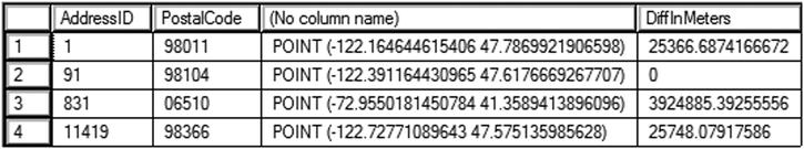
Figure 16-18. The results of using the GEOGRAPHY data type
Viewing the Spatial Results Tab
When you select GEOMETRY or GEOGRAPHY data in the native binary format, another tab shows up in the results. This tab displays a visual representation of the spatial data. Type in and execute Listing 16-12 to see how this works.
Listing 16-12. Viewing Spatial Results
--1
DECLARE @Area GEOMETRY;

--2
SET @Area = geometry::Parse('Polygon((1 4, 2 5, 5 2, 0 4, 1 4))'),

--3
SELECT @Area AS Area;
After running the code, click the Spatial Results tab. Figure 16-19 shows how this should look. This tab will show up whenever you return spatial data in the binary format in a grid.

Figure 16-19. The Spatial results tab
Although the spatial data types are very interesting, they also require specialized knowledge to take full advantage of them. I encourage you to learn more about this if you think your applications can benefit from these new data types.
SQL Server 2012 included a number of enhancements to both the geography and the geometry features. These new features demonstrate the increasing need for advanced spatial capabilities in relational databases. One of these new features is the introduction of circular arcs. Simply put, circular arcs allow for curved lines between any two points. You can also combine straight and curved lines for even more complex shapes. Figure 16-20 shows some examples.
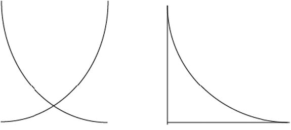
Figure 16-20. Example shapes using curved and straight lines
To create these shapes, you will use the CIRCULARSTRING command. This command requires you to define at least three points along the circular arc: a beginning, a point anywhere along the segment, and an end. The total amount of points along the arc will always be odd, and you are allowed to have the last point be the same as the first. Listing 16-13 shows how you would use the CIRCULARSTRING command to create a single curved line. You can combine multiple curved or straight lines using the COMPOUNDCURVE command. When combining lines, whether curved or straight, the beginning of the next line must always be the endpoint of the previous line. Figure 16-21 shows the output from the two SELECT statements in the listing.
Listing 16-13. Example of Curved Lines Using CIRCULARSTRING and COMPOUNDCURVE
DECLARE @g geometry;

SET @g = geometry:: STGeomFromText('CIRCULARSTRING(1 2, 2 1, 4 3)', 0);
SELECT @g.ToString();

SET @g = geometry::STGeomFromText('
COMPOUNDCURVE(
CIRCULARSTRING(1 2, 2 1, 4 3),
CIRCULARSTRING(4 3, 3 4, 1 2))', 0);
SELECT @g AS Area;
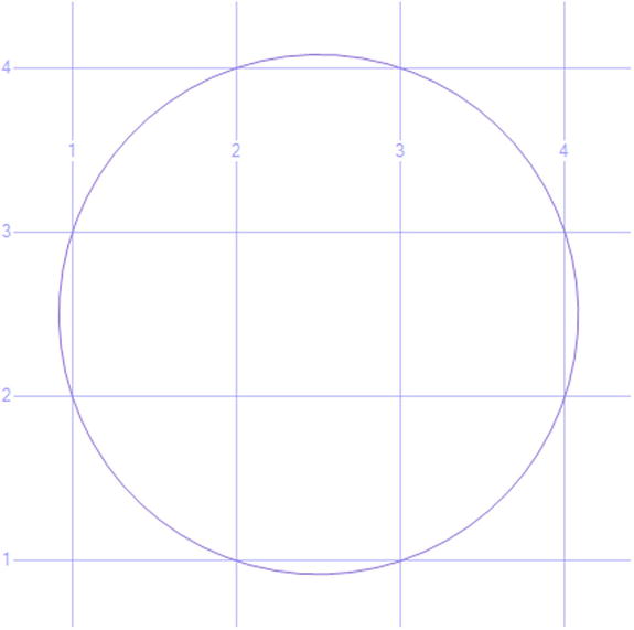
Figure 16-21. Results of using CIRCULARSTRING and COMPOUNDCURVE
The COMPOUNDCURVE command allows you to simply combine multiple curved arcs or create more complicated shapes by combining curved and straight lines. The CIRCULARSTRING command defines each circular arc while the straight lines are defined with only the points along the line. Remember that lines are defined with only two points, but curved lines are defined with three. The endpoint of one arc is the starting point of the next. Listing 16-14 shows examples of each. The shape the query generates is shown in Figure 16-22.
Listing 16-14. Example of Mixing Straight and Curved Lines Using COMPOUNDCURVE
DECLARE @g geometry = 'COMPOUNDCURVE(CIRCULARSTRING(2 0, 0 2, -2 0), (-2 0, 2 0))';
SELECT @g;

Figure 16-22. Using COMPOUNDCURVE to mix lines and curved segments
![]() Note This chapter only scratches the surface of the available features included in SQL Server for the geography and geometry data types. SQL Server includes a large number of additional methods and performance improvement for these data types such as FULLGLOBE and GEOGRAPHY_AUTO_GRID. If your job requires you to understand more on this subject or if you are simply curious, I suggest you go to http://msdn.microsoft.com/en-us/library/ff848797(v=SQL.120).aspx for more information.
Note This chapter only scratches the surface of the available features included in SQL Server for the geography and geometry data types. SQL Server includes a large number of additional methods and performance improvement for these data types such as FULLGLOBE and GEOGRAPHY_AUTO_GRID. If your job requires you to understand more on this subject or if you are simply curious, I suggest you go to http://msdn.microsoft.com/en-us/library/ff848797(v=SQL.120).aspx for more information.
Whenever you store fixed-length data, such as any of the numeric data types and some of the string data types, the data takes up the same amount of space in the database even when storing NULL values. By using the new sparse option, you can significantly reduce the amount of storage for NULL values. The tradeoff is that the non-NULL values of sparse columns take up slightly more space than values stored in regular columns, and there is a small performance decrease when retrieving the non-NULL values. To use sparse columns, the option must be specified when creating the table. You can also include a special type of column, called a column set, to return all the sparse columns as XML. Type in and execute Listing 16-15 to learn more.
Listing 16-15. Using Sparse Columns
USE tempdb;
GO

--1
IF OBJECT_ID('dbo.SparseData') IS NOT NULL BEGIN
    DROP TABLE dbo.SparseData;
END;
GO

--2
CREATE TABLE dbo.SparseData
    (ID INT NOT NULL PRIMARY KEY,
    sc1 INT SPARSE NULL,
    sc2 INT SPARSE NULL,
    sc3 INT SPARSE NULL,
    cs XML COLUMN_SET FOR ALL_SPARSE_COLUMNS);
GO

--3
INSERT INTO dbo.SparseData(ID,sc1,sc2,sc3)
VALUES  (1,1,NULL,3),(2,NULL,1,1),(3,NULL,NULL,1);

--4
INSERT INTO SparseData(ID,cs)
SELECT 4,'<sc2>5</sc2>';

--5
SELECT * FROM dbo.SparseData;

--6
SELECT ID, sc1, sc2, sc3, cs FROM SparseData;
Figure 16-23 shows the results of running this code. Code section 1 drops the dbo.SparseData table if it exists. Statement 2 creates the table with a primary key column, ID; three sparse integer columns; and the XML column, cs. Statement 3 inserts three rows into the table, leaving out the cs column. Statement 4 inserts a row, but this time only providing values for ID and cs. Query 5 uses the asterisks to return all the columns and rows with surprising results. Instead of returning the individual sparse columns, the cs column provides the sparse data. Query 6 shows that you can still retrieve these columns individually if you need to and validates the cs column. Statement 4 provides a value only for the cs column and not the sparse columns. Query 6 proves that statement 4 inserted the data correctly into the sparse column.
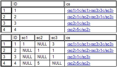
Figure 16-23. The results of using sparse columns
Because there is increased overhead when using sparse columns and because non-NULL values of sparse columns take a bit more space, Microsoft suggests that you use this feature only when the data will contain mostly NULL values. SQL Server Books Online contains a table in the “Using Sparse Columns” article showing the percentage of NULL values the data should contain in order to make using the sparse columns beneficial.
To make it easier to work with the new sparse columns, Microsoft introduced a type of index called a filtered index. By using a filtered index, you can filter out the NULL values from the sparse columns right in the index.
Thinking About Performance
SQL Server provides a multitude of data types including the special data types covered in this chapter. Choosing the correct data types can directly affect performance and storage efficiency of the database. I once had to troubleshoot issues with a database that had one data type in the entire database—VARCHAR(MAX). Just because that data type could store all the data in the database did not mean that it was a good idea.
One area in particular that can cause difficult-to-track-down performance problems is comparing expressions of different data types. The database engine sometimes must convert one side of the expression so that the values can be compared. For example, a string cannot be compared to a number without converting the string to a number. When the conversion is part of a query, it is called an explicit conversion. Otherwise it is called an implicit conversion. Either way, converting a column can cause an index to be scanned as any other function can do.
You can see the implicit conversion in the execution plan. Listing 16-16 shows an example. Be sure to turn on the Include Actual Execution Plan setting before running statements 2 and 3.
Listing 16-16. Implicit Conversions
USE AdventureWorks;
GO

--1
CREATE TABLE #Test(ID VARCHAR(20) PRIMARY KEY, LastName VARCHAR(25), FirstName VARCHAR(25));
CREATE INDEX ndxTest ON #Test(LastName);

INSERT INTO #Test(ID, LastName, FirstName)
SELECT BusinessEntityID, LastName, FirstName
FROM Person.Person;

--2
SELECT ID
FROM #Test
WHERE ID = 285;

--3
SELECT ID
FROM #Test
WHERE ID = '285';
When you look at the execution plans for statements 2 and 3, you will see that statement 2 performs an index scan and statement 3 performs an index seek. Hold the mouse cursor over the index scan operator to see the properties (Figure 16-24). The Predicate property shows the implicit conversion that causes the problem. SQL Server implicitly converted the ID value in every row to a number before comparing it to the number 285.
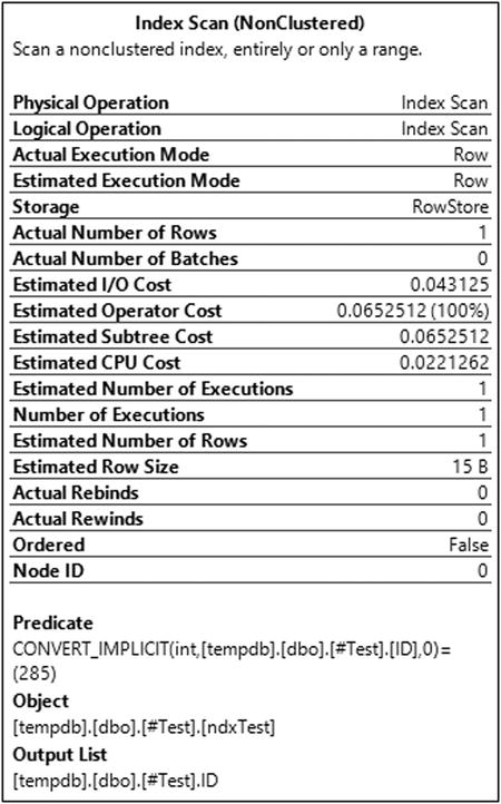
Figure 16-24. The properties of the scan
Keep data type incompatibilities in mind when troubleshooting performance issues.
Summary
By practicing the skills taught in Chapters 1 through 15, you should become a very proficient T-SQL developer. This chapter introduced you to advanced data types available in SQL Server and how to work with them. You now know that you should not use TEXT, NTEXT, and IMAGE types going forward and that the new MAX data types should be used for very large columns. If you must store files, such as Microsoft Word documents or video, you know about the FILESTREAM and FILETABLE options. The new HIERARCHYID type and the spatial types of GEOGRAPHY and GEOMETRY are available for special-purpose applications. You also have a new way to save space when working with tables that have many columns containing mostly NULLs. You now know what these types can do as well as the downsides of using these types. Armed with this knowledge, you can come up with solutions to challenging problems that may not occur to others on your team.
In Chapter 17 you will learn how to run SQL Server in the cloud!