![]()
Grouping and Summarizing Data
So far, you have learned to write simple queries that include filtering and ordering. You can also work with expressions built with operators and functions. Chapters 5 and 6 taught you how to write queries with multiple tables so that the data makes sense in applications and reports. Now it’s time to learn about a special type of query, aggregate queries, used to group and summarize data. You may find that writing aggregate queries is more challenging than the other queries you have learned so far, but by taking a step-by-step approach, you will see that they are not difficult to write at all. Be sure to take the time to understand the examples and complete all the exercises before moving on to the next section.
Aggregate Functions
You use aggregate functions to summarize data in queries. The functions that you worked with in Chapter 4 operate on one value at a time. These functions operate on sets of values from multiple rows all at once. For example, you may need to supply information about how many orders were placed and the total amount ordered for a report. Here are the most commonly used aggregate functions:
- COUNT: Counts the number of rows or the number of non-NULL values in a column.
- SUM: Adds up the values in numeric or money data.
- AVG: Calculates the average in numeric or money data.
- MIN: Finds the lowest value in the set of values. This can be used on string data as well as numeric, money, or date data.
- MAX: Finds the highest value in the set of values. This can be used on string data as well as numeric, money, or date data.
Keep the following in mind when working with these aggregate functions:
- The functions AVG and SUM will operate only on numeric and money data columns.
- The functions MIN, MAX, and COUNT will work on numeric, money, string, and temporal data columns.
- The aggregate functions will not operate on TEXT, NTEXT, and IMAGE columns. These data types are deprecated, meaning that they may not be supported in future versions of SQL Server. If you are stuck with these data types for now, you may be able to cast to a supported data type.
- The aggregate functions will not operate on some special data types like HierarchyID and spatial.
- The aggregate functions will not work on BIT columns except for COUNT. You can always cast a BIT to an INT if you need to.
- COUNT can be used with an asterisk (*) to give a count of all the rows.
- The aggregate functions ignore NULL values except for the case of COUNT(*). Using the typical settings, you will see a warning about NULLs.
- Once any aspect of aggregate queries are used in a query, the query becomes an aggregate query.
Here is the syntax for the simplest type of aggregate query where the aggregate function is used in the SELECT list:
SELECT <aggregate function>(<col1>)
FROM <table>
Listing 7-1 shows an example of using aggregate functions. Type in and execute the code to learn how these functions are used over the entire result set.
Listing 7-1. Using Aggregate Functions
--1
SELECT COUNT(*) AS CountOfRows,
    MAX(TotalDue) AS MaxTotal,
    MIN(TotalDue) AS MinTotal,
    SUM(TotalDue) AS SumOfTotal,
    AVG(TotalDue) AS AvgTotal
FROM Sales.SalesOrderHeader;

--2
SELECT MIN(Name) AS MinName,
    MAX(Name) AS MaxName,
    MIN(SellStartDate) AS MinSellStartDate
FROM Production.Product;

--3
SELECT COUNT(*) AS CountOfRows,
    COUNT(Color) AS CountOfColor,
        COUNT(DISTINCT Color) AS CountOfDistinctColor
FROM Production.Product;
Take a look at the results of running this in Figure 7-1. The aggregate functions operate on all the rows in the Sales.SalesOrderHeader table in query 1 and return just one row of results. The first expression, CountOfRows, uses an asterisk (*) to count all the rows in the table. The other expressions perform calculations on the TotalDue column. Query 2 demonstrates using the MIN and MAX functions on string and date columns. Query 3 demonstrates the three ways to use COUNT. You can count the rows, count the non-NULL value of a column, or count the distinct values of a column. In these examples, the SELECT clause lists only aggregate expressions. You will learn how to add columns that are not part of aggregate expressions in the next section.

Figure 7-1. The results of using aggregate functions
Now that you know how to use aggregate functions to summarize a result set, practice what you have learned by completing Exercise 7-1.
Use the AdventureWorks database to complete this exercise. You can find the solutions at the end of the chapter.
- Write a query to determine the number of customers in the Sales.Customer table.
- Write a query that retrieves the total number of products ordered. Use the OrderQty column of the Sales.SalesOrderDetail table and the SUM function.
- Write a query to determine the price of the most expensive product ordered. Use the UnitPrice column of the Sales.SalesOrderDetail table.
- Write a query to determine the average freight amount in the Sales.SalesOrderHeader table.
- Write a query using the Production.Product table that displays the minimum, maximum, and average ListPrice.
The GROUP BY Clause
The previous example queries and exercise questions listed only aggregate expressions in the SELECT list. The aggregate functions operated on the entire result set in each query. By adding more nonaggregated columns to the SELECT list, you add grouping levels to the query, which requires the use of the GROUP BY clause. The aggregate functions then operate on the grouping levels instead of on the entire set of results. This section covers grouping on columns and grouping on scalar expressions.
Grouping on Columns
You can use the GROUP BY clause to group data so the aggregate functions apply to groups of values instead of the entire result set. For example, you may want to calculate the count and sum of the orders placed, grouped by order date or grouped by customer. Here is the syntax for the GROUP BY clause:
SELECT <aggregate function>(<col1>), <col2>
FROM <table>
GROUP BY <col2>
One big difference you will notice once the query contains a GROUP BY clause is that additional nonaggregated columns may be included in the SELECT list. Once nonaggregated columns are in the SELECT list, you must add the GROUP BY clause and include all the nonaggregated columns. Run this code example and you will see an error message:
SELECT CustomerID,SUM(TotalDue) AS TotalPerCustomer
FROM Sales.SalesOrderHeader;
Figure 7-2 shows the error message. To get around this error, add the GROUP BY clause and include nonaggregated columns in that clause. Make sure that the SELECT list includes only those columns you really need in the results, because the SELECT list directly affects which columns will be required in the GROUP BY clause and the results of the query.
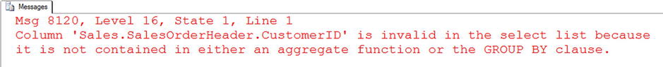
Figure 7-2. The error message that results when the required GROUP BY clause is missing
Type in and execute the code in Listing 7-2, which demonstrates how to use GROUP BY.
Listing 7-2. Using the GROUP BY Clause
--1
SELECT CustomerID,SUM(TotalDue) AS TotalPerCustomer
FROM Sales.SalesOrderHeader
GROUP BY CustomerID;

--2
SELECT TerritoryID,AVG(TotalDue) AS AveragePerTerritory
FROM Sales.SalesOrderHeader
GROUP BY TerritoryID;
Take a look at the results of running this code in Figure 7-3. Query 1 displays every customer with orders along with the sum of the TotalDue for each customer. The results are grouped by the CustomerID, and the sum is applied over each group of rows. Query 2 returns the average of the TotalDue values grouped by the TerritoryID. In each case, the nonaggregated column in the SELECT list must appear in the GROUP BY clause.
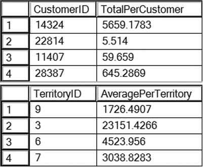
Figure 7-3. The partial results of using the GROUP BY clause
Any columns listed that are not part of an aggregate expression must be used to group the results. Those columns must be included in the GROUP BY clause. If you don’t want to group on a column, don’t list it in the SELECT list. This is where developers struggle when writing aggregate queries, so I can’t stress this enough.
Grouping on Expressions
The previous examples demonstrated how to group on columns, but it is possible to also group on scalar expressions. You must include the exact expression from the SELECT list in the GROUP BY clause. Listing 7-3 demonstrates how to avoid this mistake caused by adding a column instead of the expression to the GROUP BY clause.
Listing 7-3. How to Group on an Expression
--1
SELECT COUNT(*) AS CountOfOrders, YEAR(OrderDate) AS OrderYear
FROM Sales.SalesOrderHeader
GROUP BY OrderDate;

--2
SELECT COUNT(*) AS CountOfOrders, YEAR(OrderDate) AS OrderYear
FROM Sales.SalesOrderHeader
GROUP BY YEAR(OrderDate);
You can find the results of this code in Figure 7-4. Notice that query 1 will run, but instead of returning one row per year, the query returns multiple rows with unexpected values. Because the GROUP BY clause contains OrderDate, the grouping is on OrderDate. The CountOfOrders expression is the count by OrderDate, not OrderYear. The expression in the SELECT list just changes how the data displays; it doesn’t affect the calculations.
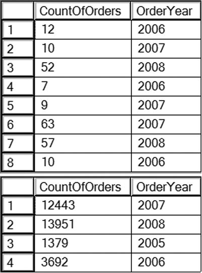
Figure 7-4. Using an expression in the GROUP BY clause
Query 2 fixes this problem by including the exact expression from the SELECT list in the GROUP BY clause. Query 2 returns only one row per year, and CountOfOrders is correctly calculated.
You use aggregate functions along with the GROUP BY clause to summarize data over groups of rows. Be sure to practice what you have learned by completing Exercise 7-2.
Use the AdventureWorks database to complete the exercise. You can find the solutions at the end of the chapter.
- Write a query that shows the total number of items ordered for each product. Use the Sales.SalesOrderDetail table to write the query.
- Write a query using the Sales.SalesOrderDetail table that displays a count of the detail lines for each SalesOrderID.
- Write a query using the Production.Product table that lists a count of the products in each product line.
- Write a query that displays the count of orders placed by year for each customer using the Sales.SalesOrderHeader table.
You already know how to use the ORDER BY clause, but special rules exist for using the ORDER BY clause in aggregate queries. If a nonaggregate column appears in the ORDER BY clause, it must also appear in the GROUP BY clause, just like the SELECT list. Here is the syntax:
SELECT <aggregate function>(<col1>),<col2>
FROM <table1>
GROUP BY <col2>
ORDER BY <col2>
Type in the following code to see the error that results when a column included in the ORDER BY clause is missing from the GROUP BY clause:
SELECT CustomerID,SUM(TotalDue) AS TotalPerCustomer
FROM Sales.SalesOrderHeader
GROUP BY CustomerID
ORDER BY TerritoryID;
Figure 7-5 shows the error message that results from running the code. To avoid this error, make sure you add only those columns to the ORDER BY clause that you intend to be grouping levels.
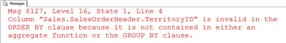
Figure 7-5. The error message resulting from including a column in the ORDER BY clause that is not a grouping level
Listing 7-4 demonstrates how to use the ORDER BY clause within an aggregate query. Be sure to type in and execute the code.
Listing 7-4. Using ORDER BY
--1
SELECT CustomerID,SUM(TotalDue) AS TotalPerCustomer
FROM Sales.SalesOrderHeader
GROUP BY CustomerID
ORDER BY CustomerID;

--2
SELECT CustomerID,SUM(TotalDue) AS TotalPerCustomer
FROM Sales.SalesOrderHeader
GROUP BY CustomerID
ORDER BY MAX(TotalDue) DESC;

--3
SELECT CustomerID,SUM(TotalDue) AS TotalPerCustomer
FROM Sales.SalesOrderHeader
GROUP BY CustomerID
ORDER BY TotalPerCustomer DESC;
View the results of Listing 7-4 in Figure 7-6. As you can see, the ORDER BY clause follows the same rules as the SELECT list. Query 1 queries the results in the order of the nonaggregated column that is listed in the GROUP BY clause. Query 2 displays the results in order of the maximum order per customer, an expression not even listed in the SELECT list. As long as it is an aggregate expression, it will work in the ORDER BY clause. Query 3 shows a nice shortcut. If you want to sort by one of the aggregate expressions in the SELECT list, you can list the alias instead of the expression.
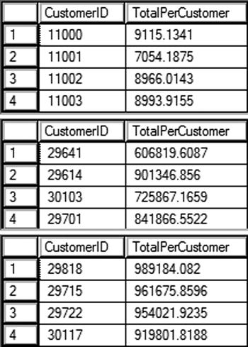
Figure 7-6. Partial results of using ORDER BY
The WHERE Clause
The WHERE clause in an aggregate query may contain anything allowed in the WHERE clause in any other query type. It may not, however, contain an aggregate expression. You use the WHERE clause to eliminate rows before the groupings and aggregates are applied. To filter after the groupings are applied, you will use the HAVING clause. You’ll learn about HAVING in the next section. Type in and execute the code in Listing 7-5, which demonstrates using the WHERE clause in an aggregate query.
Listing 7-5. Using the WHERE Clause
SELECT CustomerID,SUM(TotalDue) AS TotalPerCustomer
FROM Sales.SalesOrderHeader
WHERE TerritoryID in (5,6)
GROUP BY CustomerID;
The results shown in Figure 7-7 contain only those rows where the TerritoryID is either 5 or 6. The query eliminates the rows before the grouping is applied. Notice that TerritoryID doesn’t appear anywhere in the query except for the WHERE clause. The WHERE clause may contain any of the columns in the table as long as it doesn’t contain an aggregate expression.
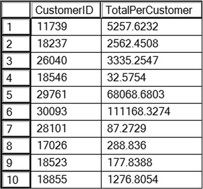
Figure 7-7. The partial results of using the WHERE clause in an aggregate query
The HAVING Clause
To eliminate rows based on an aggregate expression, use the HAVING clause. The HAVING clause may contain aggregate expressions that may or may not appear in the SELECT list. For example, you could write a query that returns the sum of the total due for customers who have placed at least ten orders. The count of the orders doesn’t have to appear in the SELECT list. Alternately, you could include only those customers who have spent at least $10,000 (sum of total due), which does appear in the list.
You can also include nonaggregated columns in the HAVING clause as long as the columns appear in the GROUP BY clause. In other words, you can eliminate some of the groups with the HAVING clause. Behind the scenes, however, the database engine may move those criteria to the WHERE clause because it is more efficient to eliminate those rows first. Criteria involving nonaggregate columns actually belong in the WHERE clause, but the query will still work with the criteria appearing in the HAVING clause.
The operators such as equal to (=), less than (<), and BETWEEN that are used in the WHERE clause will work. Here is the syntax:
SELECT <aggregate function1>(<col1>),<col2>
FROM <table1>
GROUP BY <col2>
HAVING <aggregate function2>(<col3>) = <value>
Like the GROUP BY clause, the HAVING clause will be in aggregate queries only. Listing 7-6 demonstrates the HAVING clause. Be sure to type in and execute the code.
Listing 7-6. Using the HAVING Clause
--1
SELECT CustomerID,SUM(TotalDue) AS TotalPerCustomer
FROM Sales.SalesOrderHeader
GROUP BY CustomerID
HAVING SUM(TotalDue) > 5000;

--2
SELECT CustomerID,SUM(TotalDue) AS TotalPerCustomer
FROM Sales.SalesOrderHeader
GROUP BY CustomerID
HAVING COUNT(*) = 10 AND SUM(TotalDue) > 5000;

--3
SELECT CustomerID,SUM(TotalDue) AS TotalPerCustomer
FROM Sales.SalesOrderHeader
GROUP BY CustomerID
HAVING CustomerID > 27858;
You can find the results of running this code in Figure 7-8. Query 1 shows only the rows where the sum of the TotalDue exceeds 5,000. The TotalDue column appears within an aggregate expression in the SELECT list. Query 2 demonstrates how an aggregate expression not included in the SELECT list may be used (in this case, the count of the rows) in the HAVING clause. Query 3 contains a nonaggregated column, CustomerID, in the HAVING clause, but it is a column in the GROUP BY clause. In this case, you could have moved the criteria to the WHERE clause instead and received the same results.
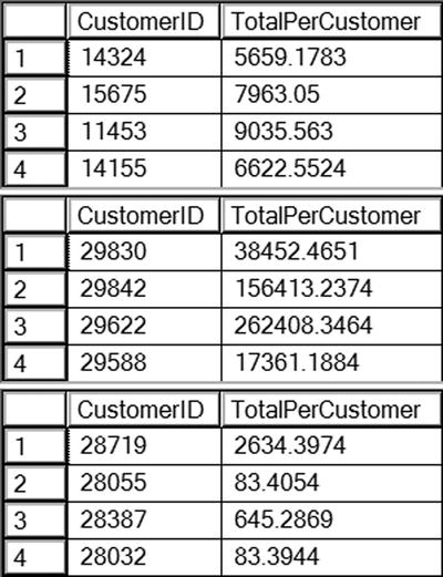
Figure 7-8. The partial results of using the HAVING clause
Developers often struggle when trying to figure out whether the filter criteria belong in the WHERE clause or in the HAVING clause. Here’s a tip: you must know the order in which the database engine processes the clauses. First, review the order in which you write the clauses in an aggregate query.
- SELECT
- FROM
- WHERE
- GROUP BY
- HAVING
- ORDER BY
The database engine processes the WHERE clause before the groupings and aggregates are applied. Here is a very simplified version of the order that the database engine actually processes the query:
- FROM
- WHERE
- GROUP BY
- HAVING
- SELECT
- ORDER BY
The database engine processes the WHERE clause before it processes the groupings and aggregates. Use the WHERE clause to completely eliminate rows from the query. For example, your query might eliminate all the orders except those placed in 2011. The database engine processes the HAVING clause after it processes the groupings and aggregates. Use the HAVING clause to eliminate rows based on aggregate expressions or groupings. For example, use the HAVING clause to remove the customers who have placed fewer than ten orders. Practice what you have learned about the HAVING clause by completing Exercise 7-3.
Use the AdventureWorks to complete this exercise. You can find the solutions at the end of the chapter.
- Write a query that returns a count of detail lines in the Sales.SalesOrderDetail table by SalesOrderID. Include only those sales that have more than three detail lines.
- Write a query that creates a sum of the LineTotal in the Sales.SalesOrderDetail table grouped by the SalesOrderID. Include only those rows where the sum exceeds 1,000.
- Write a query that groups the products by ProductModelID along with a count. Display the rows that have a count that equals 1.
- Change the query in question 3 so that only the products with the color blue or red are included.
DISTINCT Keyword
You can use the keyword DISTINCT in any SELECT list. For example, you can use DISTINCT to eliminate duplicate rows in a regular query. This section discusses using DISTINCT and aggregate queries.
Using DISTINCT vs. GROUP BY
Developers often use the DISTINCT keyword to eliminate duplicate rows from a regular query. Be careful when tempted to do this; using DISTINCT to eliminate duplicate rows may be a sign that there is a problem with the query. Assuming that the duplicate results are valid, you will get the same results by using GROUP BY instead. Type in and execute the code in Listing 7-7 to see how this works.
Listing 7-7. Using DISTINCT and GROUP BY
--1
SELECT DISTINCT SalesOrderID
FROM Sales.SalesOrderDetail;

--2
SELECT SalesOrderID
FROM Sales.SalesOrderDetail
GROUP BY SalesOrderID;
Queries 1 and 2 return identical results (see Figure 7-9). Even though query 2 contains no aggregate expressions, it is still an aggregate query because GROUP BY has been added. By grouping on SalesOrderID, only the unique values show up in the returned rows. You may be wondering which method is the best. SQL Server will generally use the same execution plan for the two techniques. Some experienced people say that, because you really don’t intend to have an aggregate query, you should avoid GROUP BY in this situation. Some say that DISTINCT should always be avoided. Really, in this case, it is up to you.
Figure 7-9. The partial results of DISTINCT vs. GROUP BY
DISTINCT Within an Aggregate Expression
You may also use DISTINCT within an aggregate query to cause the aggregate functions to operate on unique values. For example, instead of the count of rows, you could write a query that counts the number of unique values in a column. Type in and execute the code in Listing 7-8 to see how this works.
Listing 7-8. Using DISTINCT in an Aggregate Expression
--1
SELECT COUNT(*) AS CountOfRows,
    COUNT(SalesPersonID) AS CountOfSalesPeople,
    COUNT(DISTINCT SalesPersonID) AS CountOfUniqueSalesPeople
FROM Sales.SalesOrderHeader;

--2
SELECT SUM(TotalDue) AS TotalOfAllOrders,
    SUM(Distinct TotalDue) AS TotalOfDistinctTotalDue
FROM Sales.SalesOrderHeader;
Take a look at the results of running this code in Figure 7-10. Query 1 contains three aggregate expressions all using COUNT. The first one counts all rows in the table. The second expression counts the values in SalesPersonID. The expression returns a much smaller value because the data contains many NULL values, which are ignored by the aggregate function. Finally, the third expression returns the count of unique SalesPersonID values by using the DISTINCT keyword.
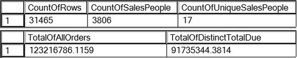
Figure 7-10. Using DISTINCT in an aggregate expression
Query 2 demonstrates that DISTINCT works with other aggregate functions, not just COUNT. The first expression returns the sum of TotalDue for all rows in the table. The second expression returns the sum of unique TotalDue values.
You can use DISTINCT either to return unique rows from your query or to make your aggregate expression operate on unique values in your data. Practice what you have learned by completing Exercise 7-4.
Use the AdventureWorks database to complete this exercise. You can find the solutions at the end of the chapter.
- Write a query using the Sales.SalesOrderDetail table to come up with a count of unique ProductID values that have been ordered.
- Write a query using the Sales.SalesOrderHeader table that returns the count of unique TerritoryID values per customer.
Aggregate Queries with More Than One Table
So far, the examples have demonstrated how to write aggregate queries involving just one table. You may use aggregate expressions and the GROUP BY and HAVING clauses when joining tables as well; the same rules apply. Type in and execute the code in Listing 7-9 to learn how to do this.
Listing 7-9. Writing Aggregate Queries with Two Tables
--1
SELECT c.CustomerID, c.AccountNumber, COUNT(*) AS CountOfOrders,
    SUM(TotalDue) AS SumOfTotalDue
FROM Sales.Customer AS c
INNER JOIN Sales.SalesOrderHeader AS s ON c.CustomerID = s.CustomerID
GROUP BY c.CustomerID, c.AccountNumber
ORDER BY c.CustomerID;

--2
SELECT c.CustomerID, c.AccountNumber, COUNT(*) AS CountOfOrders,
    SUM(TotalDue) AS SumOfTotalDue
FROM Sales.Customer AS c
LEFT OUTER JOIN Sales.SalesOrderHeader AS s ON c.CustomerID = s.CustomerID
GROUP BY c.CustomerID, c.AccountNumber
ORDER BY c.CustomerID;

--3
SELECT c.CustomerID, c.AccountNumber,COUNT(s.SalesOrderID) AS CountOfOrders,
    SUM(COALESCE(TotalDue,0)) AS SumOfTotalDue
FROM Sales.Customer AS c
LEFT OUTER JOIN Sales.SalesOrderHeader AS s ON c.CustomerID = s.CustomerID
GROUP BY c.CustomerID, c.AccountNumber
ORDER BY c.CustomerID;
You can see the results of running the code in Listing 7-9 in Figure 7-11. All three queries join the Sales.Customer and Sales.SalesOrderHeader tables together and attempt to count the orders placed and calculate the sum of the total due for each customer.
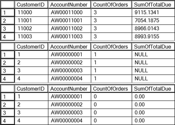
Figure 7-11. The partial results of using aggregates with multiple tables
Using an INNER JOIN, query 1 includes only the customers who have placed an order. By changing to a LEFT OUTER JOIN, query 2 includes all customers but incorrectly returns a count of 1 for customers with no orders and returns a NULL for the SumOfTotalDue when you probably want to see 0. Query 3 solves the first problem by changing COUNT(*) to COUNT(s.SalesOrderID), which eliminates the NULL values and correctly returns 0 for those customers who have not placed an order. Query 3 solves the second problem by using COALESCE to change the NULL value to 0.
Remember that writing aggregate queries with multiple tables is really not different from doing this for just one table; the same rules apply. You can use your knowledge from the previous chapters, such as how to write a WHERE clause and how to join tables, to write aggregate queries. Practice what you have learned by completing Exercise 7-5.
Use the AdventureWorks database to complete this exercise. You can find the solutions at the end of the chapter.
- Write a query joining the Person.Person, Sales.Customer, and Sales.SalesOrderHeader tables to return a list of the customer names along with a count of the orders placed.
- Write a query using the Sales.SalesOrderHeader, Sales.SalesOrderDetail, and Production.Product tables to display the total sum of products by Name and OrderDate.
Aggregate Functions and NULL
Just as you have had to consider NULL values throughout this book, you will also need to consider NULL with aggregate queries. You have seen that aggregate functions ignore NULL values. It is very important to remember this when using the AVG function. When calculating an average, do you need to consider the NULL rows? There is no right answer; it will depend on the requirements or situation. Listing 7-10 shows the difference.
Listing 7-10. Average and NULL
--1
CREATE TABLE #AvgDemo (CustID INT, OrderID INT NOT NULL, Total MONEY NOT NULL,
    DiscountAmt MONEY NULL);
INSERT INTO #AvgDemo (CustID, OrderID, Total, DiscountAmt)
SELECT CustomerID, SOD.SalesOrderID, LineTotal, NULLIF(SUM(UnitPriceDiscount * LineTotal), 0.00)
FROM sales.SalesOrderDetail AS SOD
INNER JOIN Sales.SalesOrderHeader AS SOH ON SOD.SalesOrderID = SOH.SalesOrderID
WHERE CustomerID IN (29648, 30048, 30043, 29716)
GROUP BY CustomerID, SOD.SalesOrderID, LineTotal;

--2
SELECT CustID, AVG(DiscountAmt) AS AvgDiscount,
    AVG(ISNULL(DiscountAmt,0)) AS AvgWithNullRows,
        SUM(DiscountAmt) AS SumOfDiscount,
        COUNT(*) AS CountOfRows,
        COUNT(DiscountAmt) AS NonNullCount
FROM #AvgDemo
GROUP BY CustID;
Figure 7-12 shows the results of running this code. Statement 1 creates and populates a temp table with sales information for a handful of customers. Some of the line items have discounts, but others do not. The NULLIF function is used to change zeros in the discount amount to NULL. Query 2 shows what happens when the average is calculated. The AvgDiscount uses the AVG function. Any rows with NULL in the DiscountAmt are ignored in the calculation. To get around this, you can always turn NULLs back into zeros.
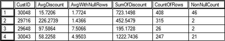
Figure 7-12. The results of testing AVG with NULLs
When you must calculate the average, and there is the possibility of NULL values, be sure to determine if the NULL rows should be ignored.
If you click the Messages tab, you will see the warning Null value is eliminated by an aggregate or other SET operation. This warning will appear with any of the aggregate functions, not just AVG. It is possible in some cases for this warning to cause errors in some applications. If this happens, one workaround is to use the SET ANSI_WARNINGS OFF setting for the connection.
Thinking About Performance
The execution plan is a great tool when you are tuning queries to get better performance. In addition, there is another tool that I use very frequently, often along with execution plans, called Statistics IO. This tool is a setting you can toggle on in the query window. Here is the command to turn this on:
SET STATISTICS IO ON;
When you turn this setting on and run queries, take a look at the Messages tab. The information will look something like that shown in Figure 7-13.
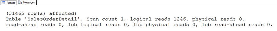
Figure 7-13. The Statistics IO information
This option provides information about how much data is read from disk and memory. Table 7-1 explains what each value means.
Table 7-1. The Output of Statistics IO
|
Item |
Meaning |
|---|---|
|
Scan count |
The number of scans or seeks. |
|
Logical reads |
The number of pages read from memory. This is the most useful value. |
|
Physical reads |
The number of pages read from disk into memory. |
|
Read-ahead reads |
The number of pages placed into cache. This number will often be inflated when an index is fragmented. |
|
Lob logical reads |
The number of pages read from memory of large object data types. |
|
Lob physical reads |
The number of pages read from disk of large object data types. |
|
Lob read-ahead |
The number of pages placed into cache of large object data types reads. |
Although it is beyond the scope of this book to cover query processing in depth, it is helpful to know a few basics. Data is stored on disk in a structure called a page. Depending on the size of each row, a page could store more than one row. For example, say that the row you need is on a page with 99 other rows. In order for SQL Server to be able to access the data, the page must be read from disk into memory. The entire page, including the 99 rows you don’t care about, must reside in memory before your row can be returned.
The physical reading of pages from disk to memory is usually the most resource-intensive part of the process and often the source of performance bottlenecks, especially if there is not enough random access memory (RAM) on the system to cache, or hold, much data. In that case, the same pages might be read over and over again each time they are needed when it would be more efficient to just hold them in cache. You might guess that among all of the information returned by Statistics IO that physical reads, the number of pages read from disk into memory, would be the most important. Instead, when tuning queries, the logical reads value is actually the one to pay attention to. The logical reads will not change from execution to execution of the identical query, unlike physical reads. This allows a level playing field when comparing two queries for performance.
When comparing the performance of two queries, the query that performs the best will have the lowest number of logical reads. Type in and run Listing 7-11 and then look at the Messages tab to see an example.
Listing 7-11. Using Statistics IO
SET STATISTICS IO ON;
GO

SELECT *
FROM Sales.SalesOrderHeader;

SELECT SalesOrderID
FROM Sales.SalesOrderHeader;

SELECT SalesOrderID, OrderDate
FROM Sales.SalesOrderHeader;
Figure 7-14 shows the Statistics IO output. You may be wondering why query 1 has 689 logical reads while query 2 has only 57. You may guess that since query 1 returns all the columns, the database engine must read more pages when accessing more columns. But in this case entire rows are stored on the pages, and SQL Server must read the entire page, not just the required columns.
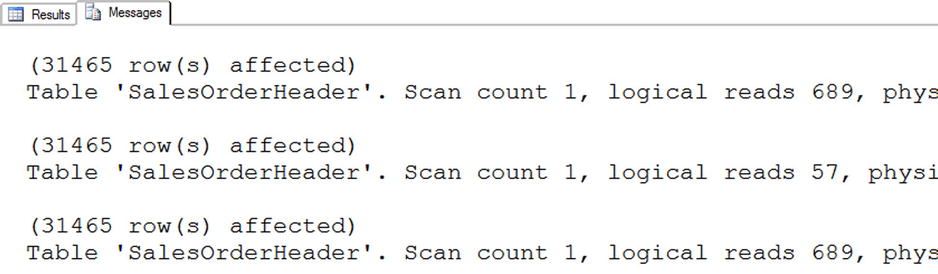
Figure 7-14. The Statistics IO output
![]() Note A new way to store data called column store was introduced with SQL Server 2012. Individual columns are stored in pages instead of rows. Microsoft also introduced In-Memory OLTP (Online Transaction Processing) with SQL Server 2014. This technology allows entire tables to be loaded into memory automatically for extremely fast data manipulation.
Note A new way to store data called column store was introduced with SQL Server 2012. Individual columns are stored in pages instead of rows. Microsoft also introduced In-Memory OLTP (Online Transaction Processing) with SQL Server 2014. This technology allows entire tables to be loaded into memory automatically for extremely fast data manipulation.
The reason that the first query has 689 logical reads is that it is a scan of the clustered index (table). The database engine must completely read every page in the index because there is no WHERE clause. The second query is a scan of one of the nonclustered indexes. Every nonclustered index automatically includes the cluster key, which is used to find the matching clustered index row. Nonclustered indexes are generally much smaller structures than the table itself, so that is why a much smaller number of pages were read.
Query 3 also requires 689 logical reads. The reason for this is that there is not a nonclustered index containing OrderDate, either as a key or an included column. Just like query 1, the entire clustered index must be scanned.
Summary
If you follow the steps outlined in the preceding sections, you will be able to write aggregate queries. With practice, you will become proficient in doing this. Keep the following rules in mind when writing an aggregate query:
- Any column not contained in an aggregate function in the SELECT list or ORDER BY clause must be part of the GROUP BY clause.
- Once an aggregate function, the GROUP BY clause, or the HAVING clause appears in a query, it is an aggregate query.
- Use the WHERE clause to filter out rows before the grouping and aggregates are applied. The WHERE clause doesn’t allow aggregate functions.
- Use the HAVING clause to filter out rows using aggregate functions.
- Don’t include anything in the SELECT list or ORDER BY clause that you don’t want as a grouping level.
Answers to the Exercises
This section provides solutions to the exercises found on writing aggregate queries.
Solutions to Exercise 7-1: Aggregate Functions
Use the AdventureWorks database to complete this exercise.
- Write a query to determine the number of customers in the Sales.Customer table.
SELECT COUNT(*) AS CountOfCustomers
FROM Sales.Customer; - Write a query that returns the total number of products ordered. Use the OrderQty column of the Sales.SalesOrderDetail table and the SUM function.
SELECT SUM(OrderQty) AS TotalProductsOrdered
FROM Sales.SalesOrderDetail; - Write a query to determine the price of the most expensive product ordered. Use the UnitPrice column of the Sales.SalesOrderDetail table.
SELECT MAX(UnitPrice) AS MostExpensivePrice
FROM Sales.SalesOrderDetail; - Write a query to determine the average freight amount in the Sales.SalesOrderHeader table.
SELECT AVG(Freight) AS AverageFreight
FROM Sales.SalesOrderHeader; - Write a query using the Production.Product table that displays the minimum, maximum, and average ListPrice.
SELECT MIN(ListPrice) AS Minimum,
MAX(ListPrice) AS Maximum,
AVG(ListPrice) AS Average
FROM Production.Product;
Solutions to Exercise 7-2: The GROUP BY Clause
Use the AdventureWorks database to complete this exercise.
- Write a query that shows the total number of items ordered for each product. Use the Sales.SalesOrderDetail table to write the query.
SELECT SUM(OrderQty) AS TotalOrdered, ProductID
FROM Sales.SalesOrderDetail
GROUP BY ProductID; - Write a query using the Sales.SalesOrderDetail table that displays a count of the detail lines for each SalesOrderID.
SELECT COUNT(*) AS CountOfOrders, SalesOrderID
FROM Sales.SalesOrderDetail
GROUP BY SalesOrderID; - Write a query using the Production.Product table that lists a count of the products in each product line.
SELECT COUNT(*) AS CountOfProducts, ProductLine
FROM Production.Product
GROUP BY ProductLine; - Write a query that displays the count of orders placed by year for each customer using the Sales.SalesOrderHeader table.
SELECT CustomerID, COUNT(*) AS CountOfSales,
YEAR(OrderDate) AS OrderYear
FROM Sales.SalesOrderHeader
GROUP BY CustomerID, YEAR(OrderDate);
Solutions to Exercise 7-3: The HAVING Clause
Use the AdventureWorks database to complete this exercise.
- Write a query that returns a count of detail lines in the Sales.SalesOrderDetail table by SalesOrderID. Include only those sales that have more than three detail lines.
SELECT COUNT(*) AS CountOfDetailLines, SalesOrderID
FROM Sales.SalesOrderDetail
GROUP BY SalesOrderID
HAVING COUNT(*) > 3; - Write a query that creates a sum of the LineTotal in the Sales.SalesOrderDetail table grouped by the SalesOrderID. Include only those rows where the sum exceeds 1,000.
SELECT SUM(LineTotal) AS SumOfLineTotal, SalesOrderID
FROM Sales.SalesOrderDetail
GROUP BY SalesOrderID
HAVING SUM(LineTotal) > 1000; - Write a query that groups the products by ProductModelID along with a count. Display the rows that have a count that equals 1.
SELECT ProductModelID, COUNT(*) AS CountOfProducts
FROM Production.Product
GROUP BY ProductModelID
HAVING COUNT(*) = 1; - Change the query in question 3 so that only the products with the color blue or red are included.
SELECT ProductModelID, COUNT(*) AS CountOfProducts, Color
FROM Production.Product
WHERE Color IN ('Blue','Red')
GROUP BY ProductModelID, Color
HAVING COUNT(*) = 1;
Solutions to Exercise 7-4: DISTINCT Keyword
Use the AdventureWorks database to complete this exercise.
- Write a query using the Sales.SalesOrderDetail table to come up with a count of unique ProductID values that have been ordered.
SELECT COUNT(DISTINCT ProductID) AS CountOFProductID
FROM Sales.SalesOrderDetail; - Write a query using the Sales.SalesOrderHeader table that returns the count of unique TerritoryID values per customer.
SELECT COUNT(DISTINCT TerritoryID) AS CountOfTerritoryID,
CustomerID
FROM Sales.SalesOrderHeader
GROUP BY CustomerID;
Solutions to Exercise 7-5: Aggregate Queries with More Than One Table
Use the AdventureWorks database to complete this exercise.
- Write a query joining the Person.Person, Sales.Customer, and Sales.SalesOrderHeader tables to return a list of the customer names along with a count of the orders placed.
SELECT COUNT(*) AS CountOfOrders, FirstName,
MiddleName, LastName
FROM Person.Person AS P
INNER JOIN Sales.Customer AS C ON P.BusinessEntityID = C.PersonID
INNER JOIN Sales.SalesOrderHeader
AS SOH ON C.CustomerID = SOH.CustomerID
GROUP BY FirstName, MiddleName, LastName; - Write a query using the Sales.SalesOrderHeader, Sales.SalesOrderDetail, and Production.Product tables to display the total sum of products by Name and OrderDate.
SELECT SUM(OrderQty) SumOfOrderQty, P.Name, SOH.OrderDate
FROM Sales.SalesOrderHeader AS SOH
INNER JOIN Sales.SalesOrderDetail AS SOD
ON SOH.SalesOrderID = SOD.SalesOrderDetailID
INNER JOIN Production.Product AS P ON SOD.ProductID = P.ProductID
GROUP BY P.Name, SOH.OrderDate;