
Analyzing Discrete-Time Systems in the Time Domain
Chapter Objectives
- Develop the notion of a discrete-time system.
- Learn simplifying assumptions made in the analysis of discrete-time systems. Discuss the concepts of linearity and time invariance, and their significance.
- Explore the use of difference equations for representing discrete-time systems.
- Develop methods for solving difference equations to compute the output signal of a system in response to a specified input signal.
- Learn to represent a difference equation in the form of a block diagram that can be used as the basis for simulating or realizing a system.
- Discuss the significance of the impulse response as an alternative description form for linear and time-invariant systems.
- Learn how to compute the output signal for a linear and time-invariant system using convolution. Understand the graphical interpretation of the steps involved in carrying out the convolution operation.
- Learn the concepts of causality and stability as they relate to physically realizable and usable systems.
3.1 Introduction
The definition of a discrete-time system is similar to that of its continuous-time counterpart:
In general, a discrete-time system is a mathematical formula, method or algorithm that defines a cause-effect relationship between a set of discrete-time input signals and a set of discrete-time output signals.
Signal-system interaction involving a single-input single-output discrete-time system is illustrated in Fig. 3.1.
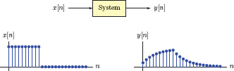
The input-output relationship of a discrete-time system may be expressed in the form
where Sys{...} represents the transformation that defines the system in the time domain. A very simple example is a system that simply multiplies its input signal by a constant gain factor K
or a system that delays its input signal by m samples
or one that produces an output signal proportional to the square of the input signal
A system with higher complexity can be defined using a difference equation that establishes the relationship between input and output signals.
Two commonly used simplifying assumptions used in studying mathematical models of systems, namely linearity and time invariance, will be the subject of Section 3.2. Section 3.3 deals with the issue of deriving a difference equation model for a discrete-time system, and Section 3.4 discusses the characteristics of constant-coefficient linear difference equations. Solution methods for constant-coefficient linear difference equations are presented in Section 3.5. Block diagrams for realizing discrete-time systems are introduced in Section 3.6. In Section 3.7 we discuss the significance of the impulse response for discrete-time systems, and its use in the context of the convolution operator for determining the output signal. Concepts of causality and stability of systems are discussed in Sections 3.8 and 3.9 respectively.
3.2 Linearity and Time Invariance
In our discussion of continuous-time systems in Chapter 2 we have relied heavily on the simplifying assumptions of linearity and time invariance. We have seen that these two assumptions allow a robust set of analysis methods to be developed. The same is true for the analysis of discrete-time systems.
3.2.1 Linearity in discrete-time systems
Linearity property will be very important as we analyze and design discrete-time systems. Conditions for linearity of a discrete-time system are:
Conditions for linearity:
Eqns. (3.5) and (3.6), referred to as the additivity rule and the homogeneity rule respectively, must be satisfied for any two discrete-time signals x1[n] and x2[n] as well as any arbitrary constant α1. These two criteria can be combined into one equation known as the superposition principle.
Superposition principle:
Verbally expressed, Eqn. (3.7) implies that the response of the system to a weighted sum of any two input signals is equal to the same weighted sum of the individual responses of the system to each of the two input signals. Fig. 3.2 illustrates this concept.
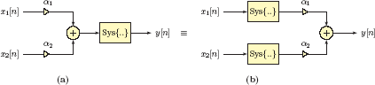
Illustration of Eqn. (3.7). The two configurations shown are equivalent if the system under consideration is linear.
A generalization of the principle of superposition for the weighted sum of N discrete-time signals is expressed as
The response of a linear system to a weighted sum of N arbitrary signals is equal to the same weighted sum of individual responses of the system to each of the N signals. Let yi[n] be the response to the input term xi[n] alone, that is yi[n] = Sys {xi[n]} for i = 1,...,N.
Superposition principle implies that
This is illustrated in Fig. 3.3.
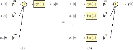
Illustration of Eqn. (3.7). The two configurations shown are equivalent if the system under consideration is linear.
Example 3.1: Testing linearity in discrete-time systems
For each of the discrete-time systems described below, determine whether the system is linear or not:
- y[n] = 3x[n] + 2x[n − 1]
- y[n] = 3x [n] + 2x [n + 1] x[n − 1]
- y[n] = a−n x[n]
Solution:
In order to test the linearity of the system we will think of its responses to the two discrete-time signals x1[n] and x2[n] as
and
The response of the system to the linear combination signal x[n] = α1x1[n] + α2x2[n] is computed as
Superposition principle holds, and therefore the system in question is linear.
Again using the test signals x1[n] and x2[n] we have
and
Use of the linear combination signal x[n] = α1x1[n] + α2x2[n] as input to the system yields the output signal
In this case the superposition principle does not hold true. The system in part (b) is therefore not linear.
The responses of the system to the two test signals are
and
and the response to the linear combination signal x[n] = α1x1[n] + α2x2[n] is
The system is linear.
3.2.2 Time invariance in discrete-time systems
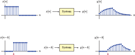
The definition of the time invariant property for a discrete-time system is similar to that of a continuous-time system. Let a discrete-time system be described with the input-output relationship y[n] = Sys{x[n]}. For the system to be considered time-invariant,the only effect of time-shifting the input signal should be to cause an equal amount of time shift in the output signal.
Condition for time invariance:
This relationship is depicted in Fig. 3.4.
Alternatively, the time-invariant nature of a system can be characterized by the equivalence of the two configurations shown in Fig. 3.5.

Another interpretation of time-invariance. The two configurations shown are equivalent for a time-invariant system.
Example 3.2: Testing time invariance in discrete-time systems
For each of the discrete-time systems described below, determine whether the system is time-invariant or not:
- y[n] = y[n − 1] + 3x[n]
- y[n] = x[n]y[n − 1]
- y[n] = nx [n − 1]
Solution:
We will test the time-invariance property of the system by time-shifting both the input and the output signals by the same number of samples, and see if the input–output relationship still holds. Replacing the index n by n − k in the arguments of all input and output terms we obtain
The input–output relationship holds, therefore the system is time-invariant.
Proceeding in a similar fashion we have
This system is time-invariant as well.
Replacing the index n by n − k in the arguments of all input and output terms yields
This system is clearly not time-invariant since the input–output relationship no longer holds after input and output signals are time-shifted.
Should we have included the factor n in the time shifting operation when we wrote the response of the system to a time-shifted input signal? In other words, should we have written the response as
The answer is no. The factor n that multiplies the input signal is part of the system definition and not part of either the input or the output signal. Therefore we cannot include it in the process of time-shifting input and output signals.
3.2.3 DTLTI systems
Discrete-time systems that are both linear and time-invariant will play an important role in the rest of this textbook. We will develop time- and frequency-domain analysis and design techniques for working with such systems. To simplify the terminology, we will use the acronym DTLTI to refer to discrete-time linear and time-invariant systems.
3.3 Difference Equations for Discrete-Time Systems
In Section 2.3 we have discussed methods of representing continuous-time systems with differential equations. Using a similar approach, discrete-time systems can be modeled with difference equations involving current, past, or future samples of input and output signals. We will begin our study of discrete-time system models based on difference equations with a few examples. Each example will start with a verbal description of a system and lead to a system model in the form of a difference equation. Some of the examples will lead to systems that will be of fundamental importance in the rest of this text while other examples lead to nonlinear or time-varying systems that we will not consider further. In the sections that follow we will focus our attention on difference equations for DTLTI systems, and develop solution techniques for them using an approach that parallels our study of differential equations for CTLTI systems.
Example 3.3: Moving-average filter
A length-N moving average filter is a simple system that produces an output equal to the arithmetic average of the most recent N samples of the input signal. Let the discrete-time output signal be y[n]. If the current sample index is 100, the current output sample y[100] would be equal to the arithmetic average of the current input sample x[100] and (N − 1) previous input samples. Mathematically we have
The general expression for the length-N moving average filter is obtained by expressing the n-th sample of the output signal in terms of the relevant samples of the input signal as
Eqn. (3.11) is a difference equation describing the input-output relationship of the moving average filter as a discrete-time system. The operation of the length-N moving average filter is best explained using the analogy of a window, as illustrated in Fig. 3.6.

Suppose that we are observing the input signal through a window that is wide enough to hold N samples of the input signal at any given time. Let the window be stationary, and let the input signal x[n] move to the left one sample at a time, similar to a film strip. The current sample of the input signal is always the rightmost sample visible through the window. The current output sample is the arithmetic average of the input samples visible through the window.
Moving average filters are used in practical applications to smooth the variations in a signal. One example is in analyzing the changes in a financial index such as the Dow Jones Industrial Average. An investor might use a moving average filter on a signal that contains the values of the index for each day. A 50-day or a 100-day moving average window may be used for producing an output signal that disregards the day-to-day fluctuations of the input signal and focuses on the slowly varying trends instead. The degree of smoothing is dependent on N, the size of the window. In general, a 100-day moving average is smoother than a 50-day moving average.
Let x[n] be the signal that holds the daily closing values of the index for the calendar year 2003. The 50-day moving averages are computed by
and 100-day moving averages are computed by
Fig. 3.7 shows the daily values of the index for the calendar year 2003 as a discrete-time signal as well as the outputs produced by 50-day and 100-day moving average filters. Note that, in the computation of the output signal samples y1[0],...,y1[48] as well as the output signal samples y2[0],...,y2[98], the averaging window had to be supplied with values from 2002 data for the index. For example, to compute the 50-day moving average on January 1 of 2003, previous 49 samples of the data from December and part of November of 2002 had to be used.
![Figure showing (a) Signal x[n] representing the Dow Jones Industrial Average daily values for the calendar year 2003, (b) the signal y1[n] holding 50-day moving average values for the index, (c) the signal y2[n] holding 100-day moving average values for the index, (d) signals x[n],y1[n] and y2[n] depicted as line graphs on the same set of axes for comparison.](http://imgdetail.ebookreading.net/data/1/9781466598546/9781466598546__signals-and-systems__9781466598546__image__193x001.png)
(a) Signal x[n] representing the Dow Jones Industrial Average daily values for the calendar year 2003, (b) the signal y1[n] holding 50-day moving average values for the index, (c) the signal y2[n] holding 100-day moving average values for the index, (d) signals x[n],y1[n] and y2[n] depicted as line graphs on the same set of axes for comparison.
We will develop better insight for the type of smoothing achieved by moving average filters when we discuss frequency domain analysis methods for discrete-time systems.
Interactive Demo: ma_demo1
The interactive demo program ma_demo1.m illustrates the length-N moving average filter discussed in Example 3.3. Because of the large number of samples involved, the two discrete-time signals are shown through line plots as opposed to stem plots. The first plot is the Dow Jones Industrial Average data for the year 2003 which is preceded by partial data from the year 2002. The second plot is the smoothed output signal of the moving average filter. The current sample index n and the length N of the moving average filter can each be specified through the user interface controls. The current sample index is marked on each plot with a red dot. Additionally, the window for the moving average filter is shown on the first plot, superimposed with the input data. The green horizontal line within the window as well as the green arrows indicate the average amplitude of the samples that fall within the window.
- Increment the sample index and observe how the window slides to the right each time. Observe that the rightmost sample in the window is the current sample, and the window accommodates a total of N samples.
- For each position of the window, the current output sample is the average of all input samples that fall within the window. Observe how the position of the window relates to the value of the current output sample.
- The length of the filter, and consequently the width of the window, relates to the degree of smoothing achieved by the moving average filter. Vary the length of the filter and observe the effect on the smoothness of the output signal.
Software resources:
ma_demo1.m
Example 3.4: Length-2 moving-average filter
A length-2 moving average filter produces an output by averaging the current input sample and the previous input sample. This action translates to a difference equation in the form
and is illustrated in Fig. 3.8. The window through which we look at the input signal accommodates two samples at any given time, and the current input sample is close to the right edge of the window. As in the previous example, we will assume that the window is stationary, and the system structure shown is also stationary. We will imagine the input signal moving to the left one sample at a time like a film strip. The output signal in the lower part of the figure also acts like a film strip and moves to the left one sample at a time, in sync with the input signal. If we wanted to write the input-output relationship of the length-2 moving average filter for several values of the index n,we would have

and so on.
Interactive Demo: ma_demo2
The interactive demo program ma_demo2.m illustrates a length-2 moving average filter discussed in Example 3.4. The input and output signals follow the film strip analogy, and can be moved by changing the current index through the user interface. Input signal samples that fall into the range of the length-2 window are shown in red color. Several choices are available for the input signal for experimentation.
- Set the input signal to a unit-impulse, and observe the output signal of the length-2 moving average filter. What is the impulse response of the system?
- Set the input signal to a unit-step, and observe the output signal of the system. Pay attention to the output samples as the input signal transitions from a sample amplitude of 0 to 1. The smoothing effect should be most visible during this transition.
Software resources:
ma_demo2.m
Example 3.5: Length-4 moving average filter
A length-4 moving average filter produces an output by averaging the current input sample and the previous three input samples. This action translates to a difference equation in the form
and is illustrated in Fig. 3.9.

For a few values of the index we can write the following set of equations:
Interactive Demo: ma_demo3
The interactive demo program ma_demo3.m illustrates a length-4 moving average filter discussed in Example 3.5. Its operation is very similar to that of the program ma_demo2.m.
- Set the input signal to a unit-impulse, and observe the output signal of the length-4 moving average filter. What is the impulse response for this system?
- Set the input signal to a unit-step, and observe the output signal of the system. Pay attention to the output samples as the input signal transitions from a sample amplitude of 0 to 1. How does the result differ from the output signal of the length-2 moving average filter in response to a unit-step?
Software resources:
ma_demo3.m
See MATLAB Exercises 3.1 and 3.2. |
Example 3.6: Exponential smoother
Another method of smoothing a discrete-time signal is through the use of an exponential smoother which employs a difference equation with feedback. The current output sample is computed as a mix of the current input sample and the previous output sample through the equation
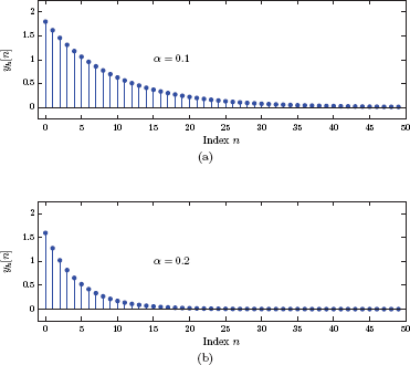
The parameter α is a constant in the range 0 < α < 1, and it controls the degree of smoothing. According to Eqn. (3.14), the current output sample y[n] has two contributors, namely the current input sample x[n] and the previous output sample y[n − 1]. The contribution of the current input sample is proportional to α, and the contribution of the previous output sample is proportional to 1 − α. Smaller values of α lead to smaller contributions from each input sample, and therefore a smoother output signal. Writing the difference equation given by Eqn. (3.14) for several values of the sample index n we obtain
and so on. Since the difference equation in Eqn. (3.14) is linear with constant coefficients, the exponential smoother would be an example of a DTLTI system provided that it is initially relaxed which, in this case, implies that y[−1] = 0. Fig. 3.10 illustrates the application of the linear exponential smoother to the 2003 Dow Jones Industrial Average data for α = 0.1 and α = 0.2.
![Figure showing Input signal x[n] representing the Dow Jones Industrial Average daily values for the calendar year 2003 compared to the output of the linear exponential smoother with (a) α = 0.1, and (b) α = 0.2.](http://imgdetail.ebookreading.net/data/1/9781466598546/9781466598546__signals-and-systems__9781466598546__image__197x001.png)
Input signal x[n] representing the Dow Jones Industrial Average daily values for the calendar year 2003 compared to the output of the linear exponential smoother with (a) α = 0.1, and (b) α = 0.2.
See MATLAB Exercise 3.3. |
Interactive Demo: es_demo
The interactive demo program es_demo.m illustrates the operation of the exponential smoother discussed in Example 3.6. The input and output signals follow the film strip analogy, and can be moved by changing the current index through the user interface. The smoothing parameter α can also be varied. Several choices are available for the input signal for experimentation.
- Set the input signal to a unit impulse, and observe the output signal of the linear exponential smoother. What is the length of the impulse response for this system?
- Vary the parameter α and observe its effect on the response to a unit impulse.
- Set the input signal to Dow Jones Industrial Average data and observe the smoothing effect as the parameter α is varied.
Software resources:
es_demo.m
A practical everyday use of a difference equation can be found in banking: borrowing money for the purchase of a house or a car. The scenario is familiar to all of us. We borrow the amount that we need to purchase that dream house or dream car, and then pay back a fixed amount for each of a number of periods, often measured in terms of months. At the end of each month the bank will compute our new balance by taking the balance of the previous month, increasing it by the monthly interest rate, and subtracting the payment we made for that month. Let y[n] represent the amount we owe at the end of the n-th month, and let x[n] represent the payment we make in month n. If c is the monthly interest rate expressed as a fraction (for example, 0.01 for a 1 percent monthly interest rate), then the loan balance may be modeled as the output signal of a system with the following difference equation as shown in Fig. 3.11:
Expressing the input-output relationship of the system through a difference equation allows us to analyze it in a number of ways. Let A represent the initial amount borrowed in month n = 0, and let the monthly payment be equal to B for months n = 1, 2,.... One method of finding y[n] would be to solve the difference equation in Eqn. (3.15) with the input signal
and the initial condition y[0] = A. Alternatively we can treat the borrowed amount as a negative payment in month 0, and solve the difference equation with the input signal
and the initial condition y[−1] = 0.
In later parts of this text, as we develop the tools we need for analysis of systems, we will revisit this example. After we learn the techniques for solving linear constant-coefficient difference equations, we will be able to find the output of this system in response to an input given by Eqn. (3.17).
Example 3.8: A nonlinear dynamics example
An interesting example of the use of difference equations is seen in chaos theory and its applications to nonlinear dynamic systems. Let the output y[n] of the system represent the population of a particular kind of species in a particular environment, for example, a certain type of plant in the rain forest. The value y[n] is normalized to be in the range 0 < y[n] < 1 with the value 1 corresponding to the maximum capacity for the species which may depend on the availability of resources such as food, water, direct sunlight, etc. In the logistic growth model, the population growth rate is assumed to be proportional to the remaining capacity 1 − y[n], and population change from one generation to the next is given by
where r is a constant. This is an example of a nonlinear system that does not have an input signal. Instead, it produces an output signal based on its initial state.
Software resources:
ex_3_8.m
Example 3.9: Newton-Raphson method for finding a root of a function
In numerical analysis, one of the simplest methods for finding the real roots of a well-behaved function is the Newton-Raphson technique. Consider a function u = f (w)shown in Fig. 3.12. Our goal is to find the value of w for which u = f (w) = 0
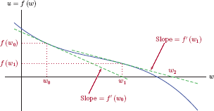
Starting with an initial guess w = w0 for the solution, we draw the line that is tangent to the function at that point, as shown in Fig. 3.12. The value w = w1 where the tangent line intersects the real axis is our next, improved, guess for the root. The slope of the tangent line is f′(w0), and it passes through the point (w0, f (w0)). Therefore, the equation of the tangent line is
At the point where the tangent line intersects the horizontal axis we have u = 0 and w = w1. Substituting these values into Eqn. (3.19) we have
and solving for w1 results in
Thus, from an initial guess w0 for the solution, we find a better guess w1 through the use of Eqn. (3.21). Repeating this process, an even closer guess can be found as
and so on. The technique can be modeled as a discrete-time system. Let the output signal y[n] represent successive guesses for the root, that is, y[n] = wn. The next successive guess can be obtained from the previous one through the difference equation
As an example of converting this procedure to a discrete-time system, let the function be
where A is any positive real number. We can write
The difference equation in Eqn. (3.23) becomes
Obviously Eqn. (3.25) represents a nonlinear difference equation. Let us use this system to iteratively find the square root of 10 which we know is . The function the root of which we are seeking is f (w) = w 2 − 10. Starting with an initial guess of y[0] = 1 we have
The next iteration produces
Continuing in this fashion we obtain y[3] = 3.196005, y[4] = 3.162456, and y[5] = 3.162278 which is accurate as the square root of 10 up to the sixth decimal digit.
Software resources:
ex_3_9.m
3.4 Constant-Coefficient Linear Difference Equations
DTLTI systems can be modeled with constant-coefficient linear difference equations. A linear difference equation is one in which current, past and perhaps even future samples of the input and the output signals can appear as linear terms. Furthermore, a constant coefficient linear difference equation is one in which the linear terms involving input and output signals appear with coefficients that are constant, independent of time or any other variable.
The moving-average filters we have explored in Examples 3.3, 3.4 and 3.5 were described by constant-coefficient linear difference equations:
A common characteristic of these three difference equations is that past or future samples of the output signal do not appear on the right side of any of them. In each of the three difference equations the output y[n] is computed as a function of current and past samples of the input signal. In contrast, reconsider the difference equation for the exponential smoother
or the difference equation for the system that computes the current balance of a loan
Both of these systems also have constant-coefficient linear difference equations (we assume that parameters α and c are constants). What sets the last two systems apart from the three moving average filters above is that they also have feedback in the form of past samples of the output appearing on the right side of the difference equation. The value of y[n] depends on the past output sample y[n − 1].
Examples 3.8 and 3.9, namely the logistic growth model and the Newton-Raphson algorithm for finding a square root, utilized the difference equations
and
Both of these difference equations are nonlinear since they contain nonlinear terms of y[n−1].
A general constant-coefficient linear difference equation representing a DTLTI system is in the form
or in closed summation form as shown below.
The order of the difference equation (and therefore the order of the system it represents) is the larger of N and M. For example, the length-2 moving average filter discussed in Example 3.4 is a first-order system. Similarly, the orders of the length-4 and the length-10 moving average filters of Examples 3.5 and 3.3 are 3 and 9 respectively.
A note of clarification is in order here: The general form we have used in Eqns. (3.26) and (3.27) includes current and past samples of x[n] and y[n] but no future samples. This is for practical purposes only. The inclusion of future samples in a difference equation for the computation of the current output would not affect the linearity and the time invariance of the system represented by that difference equation, as long as the future samples also appear as linear terms and with constant coefficients. For example, the difference equation
is still a constant-coefficient linear difference equation, and it may still correspond to a DTLTI system. We just have an additional challenge in computing the output signal through the use of this difference equation: We need to know future values of the input signal. For example, computation of y[45] requires the knowledge of x[46] and x[47] in addition to other terms. We will explore this further when we discuss the causality property later in this chapter.
Example 3.10: Checking linearity and time-invariance of a difference equation
Determine whether the first-order constant-coefficient linear difference equation in the form
represents a DTLTI system.
Solution: Our approach will be similar to that employed in Example 2.7 of Chapter 2 for a continuous-time system. Assume that two input signals x1[n] and x2[n] produce the corresponding output signals y1[n] and y2[n] respectively. Each of the signal pairs x1[n] ↔ y1[n] and x2[n] ↔ y2[n] must satisfy the difference equation, so we have
and
Let a new input signal be constructed as a linear combination of x1[n] and x2[n] as
For the system described by the difference equation to be linear, its response to the input signal x3[n] must be
and the input-output signal pair x3[n] ↔ y3[n] must also satisfy the difference equation. Substituting y3[n] into the left side of the difference equation yields
By rearranging the terms on the right side of Eqn. (3.33) we get
Substituting Eqns. (3.29) and (3.30) into Eqn. (3.34) leads to
proving that the input-output signal pair x3[n] ↔ y3[n] satisfies the difference equation.
Before we can claim that the difference equation in question represents a linear system, we need to check the initial value of y[n]. We know from previous discussion that a difference equation like the one given by Eqn. (3.29) can be solved iteratively starting at a specified value of the index n = n0 provided that the value of the output sample at index n = n0 − 1 is known. For example, let n0 = 0, and let y[n0 − 1] = y[−1] = A. Starting with the specified value of y[−1] we can determine y[0] as
Having determined the value of y[0] we can find y[1] as
and continue in this fashion. Clearly the result obtained is dependent on the initial value y[−1] = A. Since the y1[n], y2[n] and y3[n] used in the development above are all solutions of the difference equation for input signals x1[n], x2[n] and x3[n] respectively, they must each satisfy the specified initial condition, that is,
In addition, the linearity condition in Eqn. (3.32) must be satisfied for all values of the index n including n = − 1:
Thus we are compelled to conclude that the system represented by Eqn. (3.29) is linear only if y[−1] = 0. In the general case, we need y[n0− 1] = 0 if the solution is to start at index n = n0.
Our next task is to check the time-invariance property of the system described by the difference equation. If we replace the index n with n − m, Eqn. (3.29) becomes
Delaying the input signal x[n] by m samples causes the output signal y[n] to be delayed by the same amount. The system is time-invariant.
In Example 3.10 we have verified that the first-order constant-coefficient linear difference equation corresponds to a DTLTI system provided that its initial state is zero. We are now ready to generalize that result to the constant-coefficient linear difference equation of any order. Let the two input signals x1[n] and x2[n] produce the output signals y1[n] and y2[n] respectively. The input-output signal pairs x1[n] ↔ y1[n] and x2[n] ↔ y2[n] satisfy the difference equation, so we can write
and
To test linearity of the system we will construct a new input signal as a linear combination of x1[n] and x2[n]:
If the system described by the difference equation is linear, its response to the input signal x3[n] must be
We will test the input-output signal pair x3[n] ↔ y3[n] through the difference equation. Substituting y3[n] into the left side of the difference equation yields
Rearranging the terms on the right side of Eqn. (3.41) and separating them into two separate summations yields
The two summations on the right side of Eqn. (3.42) can be substituted with their equivalents from Eqns. (3.37) and (3.38), resulting in
Finally, we will combine the two summations on the right side of Eqn. (3.43) back into one summation to obtain
We conclude that the input-output signal pair x3[n] ↔ y3[n] also satisfies the difference equation. The restriction discussed in Example 3.10 regarding the initial conditions will be applicable here as well. If we are interested in finding a unique solution for n ≥ n0, then the initial values
are needed. The linearity condition given by Eqn. (3.40) must be satisfied for all values of n including index values n = n0 − 1, n0 − 2,..., n0 − N. Consequently, the system that corresponds to the difference equation in Eqn. (3.27) is linear only if all the initial conditions are zero, that is,
for k = 1,...,N. Next we need to check for time invariance. Replacing the index n with n − m in Eqn. (3.27) we get
indicating that the input-output signal pair x[n − m] ↔ y[n − m] also satisfies the difference equation. Thus, the constant-coefficient linear difference equation is time-invariant.
3.5 Solving Difference Equations
The output signal of a discrete-time system in response to a specified input signal can be determined by solving the corresponding difference equation. In some of the examples of Section 3.3 we have already experimented with one method of solving a difference equation, namely the iterative method. Consider again the difference equation for the exponential smoother of Example 3.6. By writing the difference equation for each value of the index n we were able to obtain the output signal y[n] one sample at a time. Given the initial value y[−1] of the output signal, its value for n = 0 is found by
Setting n = 1 we obtain
Repeating for n = 2 leads to
and we can continue in this fashion indefinitely. The function ss_expsmoo(..) developed in MATLAB Exercise 3.3 is an implementation of the iterative solution of this difference equation.
The iterative solution method is not limited to DTLTI systems; it can also be used for solving the difference equations of nonlinear and/or time-varying systems. Consider, for example, the nonlinear difference equation for the logistic growth model of Example 3.8. For a specified parameter value r and initial value y[−1], the output at n = 0 is
Next, y[1] is computed from y[0] as
and so on. Fig. 3.13 shows the first 50 samples of the solution obtained in this fashion for r = 3.1 and y[−1] = 0.3.

First 50 samples of the iterative solution of the difference equation for the logistic growth model.
Iterative solution of a difference equation can be also used as the basis of implementing a discrete-time system on real-time signal processing hardware. One shortcoming of this approach, however, is the lack of a complete analytical solution. Each time we iterate through the difference equation we obtain one more sample of the output signal, but we do not get an expression or a formula for computing the output for an arbitrary value of the index n. If we need to know y[1527], we must iteratively compute samples y[0] through y[1526] first.
Software resources: |
See MATLAB Exercise 3.4. |
In the rest of this section we will concentrate our efforts on developing an analytical method for solving constant-coefficient linear difference equations. Analytical solution of nonlinear and/or time-varying difference equations is generally difficult or impossible, and will not be considered further in this text.
The solution method we are about to present exhibits a lot of similarities to the method developed for solving constant-coefficient ordinary differential equations in Section 2.5. We will recognize two separate components of the output signal y[n] in the form
The term yh[n] is the solution of the homogeneous difference equation found by setting x[n] = 0 in Eqn. (3.27) for all values of n:
Thus, yh[n] is the signal at the output of the system when no input signal is applied to it. As in the continuous-time case, we will refer to yh[n] as the homogeneous solution of the difference equation or, equivalently, as the natural response of the system to which it corresponds. It depends on the structure of the system which is expressed through the set of coefficients ai for i = 0,...,N. Furthermore, it depends on the initial state of the system that is expressed through the output samples y[n0 − 1],y[n0 − 2],...,y[n0 − N]. (Recall that n0 is the beginning index for the solution; usually we will use n0 = 0.) When we discuss the stability property of DTLTI systems in Section 3.9 we will discover that, for a stable system, yh[n] approaches zero for large positive and negative values of the index n.
The second term yp[n] in Eqn. (3.46) is the part of the solution that is due to the input signal x[n] applied to the system. It is referred to as the particular solution of the difference equation. It depends on both the input signal x[n] and the internal structure of the system. It is independent of the initial state of the system. The combination of the homogeneous solution and the particular solution is referred to as the forced solution or the forced response.
3.5.1 Finding the natural response of a discrete-time system
We will begin the discussion of the solution method for solving the homogeneous equation by revisiting the linear exponential smoother first encountered in Example 3.6.
Example 3.11: Natural response of exponential smoother
Determine the natural response of the exponential smoother defined in Example 3.6 if y[−1] = 2.
Solution: The difference equation for the exponential smoother was given in Eqn. (3.6). The homogeneous difference equation is found by setting x[n] = 0:
The natural response yh[n] yet to be determined must satisfy the homogeneous difference equation. We need to start with an educated guess for the type of signal yh[n] must be, and then adjust any relevant parameters. Therefore, looking at Eqn. (3.48), we ask the question: “What type of discrete-time signal remains proportional to itself when delayed by one sample?” A possible answer is a signal in the form
where z is a yet undetermined constant. Delaying y[n] of Eqn. (3.49) by one sample we get
Substituting Eqns. (3.49) and (3.50) into the homogeneous difference equation yields
or, equivalently
which requires one of the following conditions to be true for all values of n:
- c zn = 0
- [1 − (1 − α) z−1 = 0
We cannot use the former condition since it leads to the trivial solution y[n] = czn = 0, and is obviously not very useful. Furthermore, the initial condition y[−1] = 2 cannot be satisfied using this solution. Therefore we must choose the latter condition and set z = (1 − α) to obtain
The constant c is determined based on the desired initial state of the system. We want y[−1] = 2, so we impose it as a condition on the solution found in Eqn. (3.51):
This yields c = 2(1 − α) and
The natural response found is shown in Fig. 3.14 for α =1 and α = 0.2.
The natural response of the linear exponential smoother for (a) α = 0.1, and (b)α = 0.2.
Software resources:
ex_3_11.m
Let us now consider the solution of the general homogeneous difference equation in the form
Let us start with the same initial guess that we used in Example 3.11:
Shifted versions of the prescribed homogeneous solution are
which can be expressed in the general form
Which value (or values) of z can be used in the homogeneous solution? We will find the answer by substituting Eqn. (3.53) into Eqn. (3.51):
The term czn is independent of the summation index k, and can be factored out to yield
There are two ways to satisfy Eqn. (3.55):
cz n = 0
This leads to the trivial solution y[n] = 0 for the homogeneous equation, and is therefore not very interesting. Also, we have no means of satisfying any initial conditions with this solution other than y[−i] = 0 for i = 1,..., N.
-
This is called the characteristic equation of the system. Values of z that are the solutions of the characteristic equation can be used in exponential functions as solutions of the homogeneous difference equation.
The characteristic equation:
The characteristic equation for a DTLTI system is found by starting with the homogeneous difference equation and replacing delayed versions of the output signal with the corresponding negative powers of the complex variable z.
To obtain the characteristic equation, substitute:
The characteristic equation can be written in open form as
If we want to work with non-negative powers of z, we could simply multiply both sides of the characteristic equation by zP to obtain
The polynomial on the left side of the equal sign in Eqn. (3.59) is the characteristic polynomial of the DTLTI system. Let the roots of the characteristic polynomial be z1, z2,...,zN so that Eqn. (3.59) can be written as
Any of the roots of the characteristic polynomial can be used in a signal in the form
which satisfies the homogeneous difference equation:
Furthermore, any linear combination of all valid terms in the form of Eqn. (3.61) satisfies the homogeneous difference equation as well, so we can write
The coefficients c1, c2,...,cN are determined from the initial conditions. The exponential terms in the homogeneous solution given by Eqn. (3.63) are the modes of the system. In later parts of this text we will see that the modes of a DTLTI system correspond to the poles of the system function and the eigenvalues of the state matrix.
Example 3.12: Natural response of second-order system
A second-order system is described by the difference equation
Determine the natural response of this system for n ≥ 0 subject to initial conditions
Solution: The characteristic equation is
with roots z1 = 1/2 and z2 = 1/3. Therefore the homogeneous solution of the difference equation is
for n ≥ 0. The coefficients c1 and c2 need to be determined from the initial conditions. We have
Solving Eqns. (3.64) and (3.65) yields c1 = 2 and c2 = 5. The natural response of the system is
Software resources:
ex_3_12.m
In Example 3.12 the characteristic equation obtained from the homogeneous difference equation had two distinct roots that were both real-valued, allowing the homogeneous solution to be written in the standard form of Eqn. (3.63). There are other possibilities as well. Similar to the discussion of the homogeneous differential equation in Section 2.5.3 we will consider three possible scenarios:
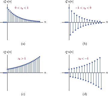
Case 1: All roots are distinct and real-valued.
This leads to the homogeneous solution
for n ≥ n0 as we have seen in Example 3.12. The value of the real root zk determines the type of contribution made to the homogeneous solution by the term . If |zk| < 1 then decays exponentially over time. Conversely, |zk| > 1 leads toa term that grows exponentially. A negative value for zk causes the corresponding term in the homogeneous solution to have alternating positive and negative sample amplitudes. Possible forms of the contribution are shown in Fig. 3.15.
Case 2: Characteristic polynomial has complex-valued roots.
Since the difference equation and its characteristic polynomial have only real-valued coefficients, any complex roots of the characteristic polynomial must appear in conjugate pairs. Therefore, if
is a complex root, then its conjugate
must also be a root. Let the part of the homogeneous solution that is due to these two roots be
The coefficients c1a and c1b are yet to be determined from the initial conditions. Since the coefficients of the difference equation are real-valued, the solution yh[n] must also be real. Furthermore, yh1 [n], the part of the solution that is due to the complex conjugate pair of roots we are considering must also be real. This implies that the coefficients c1a and c1b must form a complex conjugate pair. We will write the two coefficients in polar complex form as
Substituting Eqn. (3.68) into Eqn. (3.67) we obtain
The contribution of a complex conjugate pair of roots to the solution is in the form of a cosine signal multiplied by an exponential signal. The oscillation frequency of the discrete-time cosine signal is determined by Ω1. The magnitude of the complex conjugate roots,r1, impacts the amplitude behavior. If r1 < 1, then the amplitude of the cosine signal decays exponentially over time. If r1 > 1 on the other hand, the amplitude of the cosine signal grows exponentially over time. These two possibilities are illustrated in Fig. 3.16.
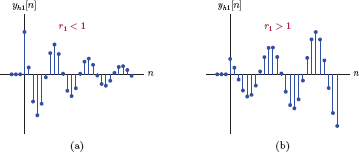
Terms corresponding to a pair of complex conjugate roots of the characteristic equation: (a) r1 < 0, (b) r1 > 1.
With the use of the the appropriate trigonometric identity1 Eqn. (3.69) can also be written in the alternative form
Case 3: Characteristic polynomial has some multiple roots.
Consider again the factored version of the characteristic equation first given by Eqn. (3.60):
What if the first two roots are equal, that is, z2 = z1? If we were to ignore the fact that the two roots are equal, we would have a natural response in the form
The equality of two roots leads to loss of one of the coefficients that we will need in order to satisfy the initial conditions. In order to gain back the coefficient we have lost, we need an additional term for the two roots at z = z1, and it can be obtained by considering a solution in the form
In general, a root of multiplicity r requires r terms in the homogeneous solution. If the characteristic polynomial has a factor (z − z1)r, the resulting homogeneous solution is
Example 3.13: Natural response of second-order system revisited
Determine the natural response of each of the second-order systems described by the difference equations below:
y[n] − 1.4y[n − 1] + 0.85y[n − 2] = 0
with initial conditions y[−1] = 5 and y[−2] = 7.
y[n] − 1.6y[n − 1] + 0.64y[n − 2] = 0
with initial conditions y[−1] = 2 and y[−2] = − 3.
The characteristic equation is
which can be solved to yield
Thus, the roots of the characteristic polynomial form a complex conjugate pair. They can be written in polar complex form as
which leads us to a homogeneous solution in the form
for n ≥ 0. The coefficients d1 and d2 need to be determined from the initial conditions. Evaluating yh[n] for n = −1 and n = − 2 we have
and
Solving Eqns. (3.74) and (3.75) yields d1 = 1.05 and d2 = −5.8583. The natural response of the system is
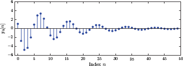
and is graphed in Fig. 3.17.
For this system the characteristic equation is
The roots of the characteristic polynomial are z1 = z2 = 0.8. Therefore we must look for a homogeneous solution in the form of Eqn. (3.72):
for n ≥ 0. Imposing the initial conditions at n = −1 and n = −2 we obtain
and
Eqns. (3.76) and (3.77) can be solved to obtain the coefficient values c1 = 5.12 and c2 = 3.52. The natural response is
and is graphed in Fig. 3.18.
Software resources:
ex_3_13a.m
ex_3_13b.m
Interactive Demo: nr_demo2
The interactive demo program nr_demo2.m illustrates different types of homogeneous solutions for a second-order discrete-time system based on the roots of the characteristic polynomial. Three possible scenarios were explored above, namely distinct real roots, complex conjugate roots and identical real roots.
In the demo program, the two roots can be specified in terms of their norms and angles using slider controls, and the corresponding natural response can be observed. If the roots are both real, then they can be controlled independently. If the roots are complex, then they move simultaneously to keep their complex conjugate relationship. The locations of the two roots z1 and z2 are marked on the complex plane. A circle with unit radius that is centered at the origin of the complex plane is also shown. The difference equation, the characteristic equation and the analytical solution for the natural response are displayed and updated as the roots are moved.
Start with two complex conjugate roots as given in part (a) of Example 3.13. Set the roots as
Set the initial values as they were set in the example, that is, y[−1] = 5 and y[−2] = 7. The natural response displayed should match the result obtained in Example 3.13.
Gradually increase the norm of the first root. Since the roots are complex, the second root will also change to keep the complex conjugate relationship of the roots. Observe the natural response as the norm of the complex roots become greater than unity and cross over the circle to the outside. What happens when the roots cross over?
Bring the norm of the roots back to z1,2 = 0.922. Gradually decrease the angle of z1. The angle of z2 will also change. How does this impact the shape of the natural response?
Set the angle of the z1 equal to zero, so that the angle of z2 also becomes zero, and the roots can be moved individually. Set the norms of the two roots as
and observe the natural response.
Gradually increase |z1| and observe the changes in the natural response, especially as the root moves outside the circle.
Software resources:
nr_demo2.m
3.5.2 Finding the forced response of a discrete-time system
In the preceding section we focused our efforts on determining the homogeneous solution of the constant-coefficient linear difference equation or, equivalently, the natural response yh[n] of the system when no external input signal exists. As stated in Eqn. (3.46), the complete solution is the sum of the homogeneous solution with the particular solution that corresponds to the input signal applied to the system. The procedure for finding a particular solution for a difference equation is similar to that employed for a differential equation. We start with an educated guess about the form of the particular solution we seek, and then adjust the values of its parameters so that the difference equation is satisfied. The form of the particular solution picked should include the input signal x[n] as well as the delayed input signals xn − k] that differ in form. For example, if the input signal is x[n] = K cos (Ω0n), then we assume a particular solution in the form
Both cosine and sine terms are needed since x[n − 1] is in the form
Other delays of x[n] do not produce any terms that differ from these. If the input signal is in the form x[n] = n m then the delays of x[n] would contain the terms nm− 1, nm−2,...,n1, n0, and the particular solution is in the form
Table 3.1 lists some of the common types of input signals and the forms of particular solutions to be used for them.
Choosing a particular solution for various discrete-time input signals.
Input signal |
Particular solution |
|---|---|
K (constant) |
k1 |
K ean |
k1 ean |
K cos (Ω0n) |
k1 cos (Ω0n) + k2 sin (Ω0n) |
K sin (Ω0n) |
k1 cos (Ω0n) + k 2 sin (Ω0n) |
K nm |
The unknown coefficients ki of the particular solution are determined from the difference equation by assuming all initial conditions are zero (recall that the particular solution does not depend on the initial conditions of the difference equation, or the initial state of the system). Initial conditions of the difference equation are imposed in the subsequent step for determining the unknown coefficients of the homogeneous solution, not the coefficients of the particular solution. The procedure for determining the complete forced solution of the difference equation is summarized below:
- Write the homogeneous difference equation, and then find the characteristic equation by replacing delays of the output signal with corresponding negative powers of the complex variable z.
- Solve for the roots of the characteristic equation and write the homogeneous solution in the form of Eqn. (3.66). If some of the roots appear as complex conjugate pairs, then use the form in Eqn. (3.70) for those roots. If there are any multiple roots, use the procedure outlined in Eqn. (3.73). Leave the homogeneous solution in parametric form with undetermined coefficients; do not attempt to compute the coefficients c1,c2,... of the homogeneous solution yet.
- Find the form of the particular solution by either picking the appropriate form of it from Table 3.1, or by constructing it as a linear combination of the input signal and its delays. (This latter approach requires that delays of the input signal produce a finite number of distinct signal forms.)
- Try the particular solution in the non-homogeneous difference equation and determine the coefficients k1, k2,... of the particular solution. At this point the particular solution should be uniquely determined. However, the coefficients of the homogeneous solution are still undetermined.
- Add the homogeneous solution and the particular solution together to obtain the total solution. Impose the necessary initial conditions and determine the coefficients c1, c2,... of the homogeneous solution.
The next two examples will illustrate these steps.
Example 3.14: Forced response of exponential smoother for unit-step input
Find the forced response of the exponential smoother of Example 3.6 when the input signal is a unit-step function, and y[−1] = 2.5.
Solution: In Example 3.11 the homogeneous solution of the difference equation for the exponential smoother was determined to be in the form
For a unit-step input, the particular solution is in the form
The particular solution must satisfy the difference equation. Substituting yp[n] into the difference equation we get
and consequently k1 = 1. The forced solution is the combination of homogeneous and particular solutions:
The constant c needs to be adjusted to satisfy the specified initial condition y[−1] = 2.5.
results in c = 1.5 (1 − α), and the forced response of the system is
This signal is shown in Fig. 3.19 for α = 0.1.

Software resources:
ex_3_14.m
Example 3.15: Forced response of exponential smoother for sinusoidal input
Find the forced response of the exponential smoother of Example 3.6 when the input signal is a sinusoidal function in the form
Use parameter values A = 20, Ω = 0.2π, and α = 0.1. The initial value of the output signal is y[−1] = 2.5.
Solution: Recall that the difference equation of the exponential smoother is
The homogeneous solution is in the form
For a sinusoidal input signal, the form of the appropriate particular solution is obtained from Table 3.1 as
The particular solution must satisfy the difference equation of the exponential smoother. Therefore we need
The term yp[n − 1] is needed in Eqn. (3.81). Time-shifting both sides of Eqn. (3.80)
Using the appropriate trigonometric identities 2 Eqn. (3.82) can be written as
Let us define
to simplify the notation. Substituting Eqns. (3.80) and (3.83) along with the input signal x[n] into the difference equation in Eqn. (3.81) we obtain
Since Eqn. (3.84) must be satisfied for all values of the index n, coefficients of cos(Ωn)and sin (Ωn) on both sides of the equal sign must individually be set equal to each other. This leads to the two equations
and
Eqns. (3.85) and (3.86) can be solved for the unknown coefficients k1 and k2 to yield
Now the forced solution of the system can be written by combining the homogeneous and particular solutions as
Using the specified parameter values of A = 20, Ω = 0.2π, α = 0.1 and β = 0.9, the coefficients k1 and k2 are evaluated to be
and the forced response of the system is
We need to impose the initial condition y[−1] = 2.5 to determine the remaining unknown coefficient c. For n = − 1 the output signal is
Solving for the coefficient c yields to c = 2.7129. The forced response can now be written in complete form:
for n ≥ 0. The forced response consists of two components. The first term in Eqn. (3.89) is the transient response
which is due to the initial state of the system. It disappears over time. The remaining terms in Eqn. (3.89) represent the steady-state response of the system:
Signals y[n], yt[n] and yss[n] are shown in Fig. 3.20.
![Figure showing the signals obtained in Example 3.15: (a) yt[n], (b) and yss[n], (c) y[n].](http://imgdetail.ebookreading.net/data/1/9781466598546/9781466598546__signals-and-systems__9781466598546__image__220x001.png)
Software resources:
ex_3_15.m
Interactive Demo: fr_demo2
The interactive demo program fr_demo2.m is based on Example 3.15, and allows experimentation with parameters of the problem. The amplitude A is fixed at A = 20 so that the input signal is
The exponential smoother parameter α, the angular frequency Ω and the initial output value y[−1] can be varied using slider controls. The effect of parameter changes on the transient response yt[n], the steady-state response yss[n] and the total forced response yt[n] + yss[n] can be observed.
- Start with the settings α = 0.1, Ω = 0.2π = 0.62832 radians, and y[−1] = 2.5. Observe the peak amplitude value of the steady-state component. Confirm that it matches with what was found in Example 3.15, Fig. 3.20.
- Now gradually increase the angular frequency Ω up to Ω = 0.5 π = 1.5708 radians, and observe the change in the peak amplitude of the steady-state component of the output. Compare with the result obtained in Eqn. (3.88).
- Set parameter values back to α = 0.1, Ω = 0.2π = 0.62832 radians, and y[−1] = 2.5. Pay attention to the transient response, and how many samples it takes for it to become negligibly small.
- Gradually decrease the value of α toward α = 0.05 and observe the changes in the transient behavior. How does the value of α impact the number of samples it takes for the output signal to reach steady state?
Software resources:
fr_demo2.m
3.6 Block Diagram Representation of Discrete-Time Systems
A discrete-time system can also be represented with a block diagram, and multiple solutions exist that are functionally equivalent. In this section we will discuss just one particular technique for obtaining a block diagram, and the discussion of other techniques will be deferred until Chapter 8.
Block diagrams are useful for discrete-time systems not only because they provide additional insight into the operation of a system, but also because they allow implementation of the system on a digital computer. We often use the block diagram as the first step in developing the computer code for implementing a discrete-time system. An example of this is given in MATLAB Exercise 3.5.
Three types of operators are utilized in the constant-coefficient linear difference equation of Eqn. (3.27): multiplication of a signal by a constant gain factor, addition of two signals, and time shift of a signal. Consequently, the fundamental building blocks for use in block diagrams of discrete-time systems are constant-gain amplifier, signal adder and one-sample delay element as shown in Fig. 3.21.

Block diagram components for discrete-time systems: (a) constant-gain amplifier, (b) one-sample delay, (c) signal adder.
We will begin the discussion with a simple third-order difference equation expressed as
This is a constant-coefficient linear difference equation in the standard form of Eqn. (3.27) with parameter values N = 3 and M = 2. Additionally, the coefficient of the term y[n] is chosen to be a0 = 1. This is not very restricting since, for the case of a0 = 1, we can always divide both sides of the difference equation by a0 to satisfy this condition. It can be shown that the following two difference equations that utilize an intermediate signal w (t) are equivalent to Eqn. (3.92):
The proof is straightforward. The terms on the right side of Eqn. (3.92) can be written using Eqn. (3.93) and its time-shifted versions. The following can be written:
We are now in a position to construct the right side of Eqn. (3.92) using Eqns. (3.95) through (3.97):
Rearranging the terms of Eqn. (3.98) we can write it in the form
and recognizing that the terms on the right side of Eqn. (3.99) are time-shifted versions of y[n] from Eqn. (3.94) we obtain
which is the original difference equation given by Eqn. (3.92). Therefore, Eqns. (3.93) and (3.94) form an equivalent representation of the system described by Eqn. (3.92).
One possible block diagram implementation of the difference equation in Eqn. (3.93) is shown in Fig. 3.22. It takes the discrete-time signal x[n] as input, and produces the intermediate signal w [n] as output.
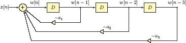
Three delay elements are used for obtaining the samples w[n − 1], w[n − 2] and w[n − 3]. The intermediate signal w[n] is then obtained via an adder that adds scaled versions of the three past samples of w[n]. Keep in mind that our ultimate goal is to obtain the signal y[n] which is related to the intermediate signal w[n] through Eqn. (3.94). The computation of y[n] requires the knowledge of w[n] as well as its two past samples w [n − 1] and w [n − 2], both of which are available in the block diagram of Fig. 3.22. The complete block diagram for the system is obtained by adding the necessary connections to the block diagram in Fig. 3.22, and is shown in Fig. 3.23.

The development above was based on a third-order difference equation, however, the extension of the technique to a general constant-coefficient linear difference equation is straightforward. In Fig. 3.23 the feed-forward gains of the block diagram are the right-side coefficients b0, b1,..., bM of the difference equation in Eqn. (3.92). Feedback gains of the block diagram are the negated left-side coefficients −a1, −a2,..., −aN of the difference equation. Recall that we must have a0 = 1 for this to work.
Imposing initial conditions
Initial conditions can easily be incorporated into the block diagram. The third-order difference equation given by Eqn. (3.92) would typically be solved subject to initial values specified for y[−1], y[−2] and y[−3]. For the block diagram we need to determine the corresponding values of w[−1], w[−2] and w[−3] through the use of Eqns. (3.93) and (3.94). This will be illustrated in Example 3.16.
Example 3.16: Block diagram for discrete-time system
Construct a block diagram to solve the difference equation
with the input signal x[n] = u[n] and subject to initial conditions
Solution: Using the intermediate variable w[n] as outlined in the preceding discussion we can write the following pair of difference equations that are equivalent to the original difference equation:
The block diagram can now be constructed as shown in Fig. 3.24.

Initial conditions specified in terms of the values of y[−1],y[−2] and y[−3] need to be translated to corresponding values of w[−1], w [−2] and w [−3]. Writing Eqn. (3.102) for n = −1, −2, −3 yields the following three equations:
These equations need to be solved for w[−1], w[−2] and w[−3]. The two additional unknowns, namely w[−4] and w[−5], need to be obtained in other ways. Writing Eqn. (3.101) for n = − 1 yields
Since x[n] = u[n] we know that x[−1] = 0, therefore w[−4] can be expressed as
which can be substituted into Eqn. (3.104) to yield
Similarly, writing Eqn. (3.101) for n = − 2 yields
We know that x [−2] = 0, therefore
Substituting Eqns. (3.107) and (3.110) into Eqn. (3.105) we obtain
Eqns. (3.103), (3.108) and (3.111) can be solved simultaneously to determine the initial conditions in terms of w[n] as
In the block diagram of Fig. 3.24 the outputs of the three delay elements should be set equal to these values before starting the simulation.
Interactive Demo: dgm_demo1
The interactive demo program dgm_demo1.m illustrates the solution of the difference equation of Example 3.16 through the use of the block diagram constructed and shown in Fig. 3.24. Two choices are given for the input signal x[n]: a unit-step signal and a periodic sawtooth signal both of which have x [−1] = x [−2] = 0. Numerical values of the node variables are shown on the block diagram. For n = 0, initial values w[n − 1] = w[−1], w[n − 2] = w[−2] and w[n − 3] = w[−3] are shown on the diagram as computed in Example 3.16.
Incrementing the sample index n by clicking the button to the right of the index field causes the node values to be updated in an animated fashion, illustrating the operation of the block diagram. Additionally, input and output samples of the system are shown as stem plots with the current samples indicated in red color.
Software resources:
dgm_demo1.m
See MATLAB Exercise 3.5. |
3.7 Impulse Response and Convolution
A constant-coefficient linear difference equation is sufficient for describing a DTLTI system such that the output signal of the system can be determined in response to any arbitrary input signal. However, we will often find it convenient to use additional description forms for DTLTI systems. One of these additional description forms is the impulse response which is simply the forced response of the system under consideration when the input signal is a unit impulse. This is illustrated in Fig. 3.25.
The impulse response also constitutes a complete description of a DTLTI system. The response of a DTLTI system to any arbitrary input signal x[n] can be uniquely determined from the knowledge of its impulse response.
In the next section we will discuss how the impulse response of a DTLTI system can be obtained from its difference equation. The reverse is also possible, and will be discussed in later chapters.
3.7.1 Finding impulse response of a DTLTI system
Finding the impulse response of a DTLTI system amounts to finding the forced response of the system when the forcing function is a unit impulse, i.e., x[n] = δ[n]. In the case of a difference equation with no feedback, the impulse response is found by direct substitution of the unit impulse input signal into the difference equation. If the difference equation has feedback, then finding an appropriate form for the particular solution may be a bit more difficult. This difficulty can be overcome by finding the unit-step response of the system as an intermediate step, and then determining the impulse response from the unit-step response.
The problem of determining the impulse response of a DTLTI system from the governing difference equation will be explored in the next two examples.
Example 3.17: Impulse response of moving average filters
Find the impulse response of the length-2, length-4 and length-N moving average filters discussed in Examples 3.3, 3.4 and 3.5.
Solution: Let us start with the length-2 moving average filter. The governing difference equation is
Let h2[n] denote the impulse response of the length-2 moving average filter (we will use the subscript to indicate the length of the window). It is easy to compute h2[n] is by setting x[n] = δ[n] in the difference equation:
The result can also be expressed in tabular form as
Similarly, for a length-4 moving average filter with the difference equation
the impulse response is
or in tabular form
These results are easily generalized to a length-N moving average filter. The difference equation of the length-N moving average filter is
Substituting x[n] = δ[n] into Eqn. (3.115) we get
The result in Eqn. (3.116) can be written in alternative forms as well. One of those alternative forms is
and another one is
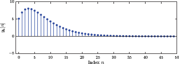
Example 3.18: Impulse response of exponential smoother
Find the impulse response of the exponential smoother of Example 3.6 with y[−1] = 0.
Solution: With the initial condition y[−1] = 0, the exponential smoother described by the difference equation in Eqn. (3.14) is linear and time-invariant (refer to the discussion in Section 3.4). These two properties will allow us to use superposition in finding its impulse response. Recall that the unit-impulse function can be expressed in terms of unit-step functions as
As a result, the impulse response of the linear exponential smoother can be found through the use of superposition in the form
We will first find the response of the system to a unit-step signal. The homogeneous solution of the difference equation at hand was already found in Example 3.11 as
For a unit-step input, the particular solution is in the form
Using this particular solution in the difference equation we get
which leads to k1 = 1. Combining the homogeneous and particular solutions, the forced solution is found to be in the form
with coefficient c yet to be determined. If we now impose the initial condition y[−1] = 0 on the result found in Eqn. (3.118) we get
and consequently
Thus, the unit-step response of the linear exponential smoother is
for n ≥ 0. In compact notation, this result can be written as
Since the system is time-invariant, its response to a delayed unit-step input is simply a delayed version of y[n] found in Eqn. (3.119):
The impulse response of the linear exponential smoother is found using Eqns. (3.119) and (3.120) as
and is shown in Fig. 3.26 for α = 0.1.

ex_3_18.m
3.7.2 Convolution operation for DTLTI systems
The development of the convolution operation for DTLTI systems will be based on the impulse decomposition of a discrete-time signal. It was established in Section 1.4.3 that any arbitrary discrete-time signal can be written as a sum of scaled and shifted impulse signals, leading to a decomposition in the form
Time-shifting a unit-impulse signal by k samples and multiplying it by the amplitude of the k-th sample of the signal x[n] produces the signal xk[n] = x[k]δ[n − k]. Repeating this process for all integer values of k and adding the resulting signals leads to Eqn. (3.122).
If x[n] is the input signal applied to a system, the output signal can be written as
The input signal is the sum of shifted and scaled impulse functions. If the system under consideration is linear, then using the additivity rule given by Eqn. (3.5) we can write
Furthermore, using the homogeneity rule given by Eqn. (3.6), Eqn. (3.124) becomes
For the sake of discussion, let us assume that we know the system under consideration to be linear, but not necessarily time-invariant. The response of the linear system to any arbitrary input signal x[n] can be computed through the use of Eqn. (3.125), provided that we already know the response of the system to impulse signals shifted in by all possible delay amounts. The knowledge necessary for determining the output of a linear system in response to an arbitrary signal x[n] is
Eqn. (3.125) provides us with a viable, albeit impractical, method of determining system output y[n] for any input signal x[n]. The amount of the prerequisite knowledge that we must possess about the system to be able to use Eqn. (3.125) diminishes its usefulness. Things improve, however, if the system under consideration is also time-invariant.
Let the impulse response of the system be defined as
If, in addition to being linear, the system is also known to be time-invariant, then the response of the system to any shifted impulse signal can be derived from the knowledge of h[n] through
consistent with the definition of time invariance given by Eqn. (3.10). This reduces the prerequisite knowledge to just the impulse response h[n], and we can compute the output signal as
Eqn. (3.128) is known as the convolution sum for discrete-time signals. The output signal y[n] of a DTLTI system is obtained by convolving the input signal x[n] and the impulse response h[n] of the system. This relationship is expressed in compact notation as
where the symbol * represents the convolution operator. We will show later in this section that the convolution operator is commutative, that is, the relationship in Eqn. (3.128) can also be written in the alternative form
by swapping the roles of h[n] and x[n] without affecting the end result.
Discrete-time convolution summary:
Example 3.19: A simple discrete-time convolution example
A discrete-time system is described through the impulse response
Use the convolution operation to find the response of the system to the input signal
Solution: Consider the convolution sum given by Eqn. (3.128). Let us express the terms inside the convolution summation, namely x[k] and h[n − k], as functions of k.
In its general form both limits of the summation in Eqn. (3.128) are infinite. On the other hand, x[k] = 0 for negative values of the summation index k, so setting the lower limit of the summation to k = 0 would have no effect on the result. Similarly, the last significant sample of x[k] is at index k = 2, so the upper limit can be changed to k =2 without affecting the result as well, leading to
If n < 0, we have h[n − k] = 0 for all terms of the summation in Eqn. (3.131), and the output amplitude is zero. Therefore we will only concern ourselves with samples for which n ≥ 0. The factor h[n − k] has significant samples in the range
which can be expressed in the alternative form
The upper limit of the summation in Eqn. (3.131) can be set equal to k = n without affecting the result, however, if n> 2 then we should leave it at k = 2. Similarly, the lower limit can be set to k = n − 3 provided that n − 3 > 0, otherwise it should be left at k = 0. So, a compact version of the convolution sum adapted to the particular signals of this example would be
where the lower limit is the larger of k = 0 and k = n − 3, and the upper limit is the smaller of k = 2 and k = n. We will use this result to compute the convolution of x[n] and h [n].
For n = 1:
For n = 2:
For n = 3:
For n = 4:
For n = 5:
Thus the convolution result is
Example 3.20: Simple discrete-time convolution example revisited
Rework the convolution problem of Example 3.19 with the following modifications applied to the two signals:
and
Assume the starting indices N1 and N2 are known constants.
Solution: We need to readjust limits of the summation index. The function x[k] has significant samples in the range
For the function h[n − k], the significant range of the index k is found from the inequality
the terms of which can be rearranged to yield
Using the inequalities in Eqns. (3.133) and (3.134) the convolution sum can be written as
with the limits
For example, suppose we have N1 = 5 and N2 = 7. Using Eqn. (3.135) with the limits in Eqn. (3.136) we can write the convolution sum as
For the summation to contain any significant terms, the lower limit must not be greater than the upper limit, that is, we need
As a result, the leftmost significant sample of y[n] will occur at index n = 12. In general, it can be shown (see Problem 3.23 at the end of this chapter) that the leftmost significant sample will be at the index n = N1 + N2. The sample y[12] is computed as
Other samples of y[n] can be computed following the procedure demonstrated in Example 3.19 and yield the same pattern of values with the only difference being the starting index. The complete solution is
Software resources: |
See MATLAB Exercise 3.7. |
In computing the convolution sum it is helpful to sketch the signals. The graphical steps involved in computing the convolution of two signals x[n] and h[n] at a specific index value n can be summarized as follows:
Sketch the signal x[k] as a function of the independent variable k. This corresponds to a simple name change on the independent variable, and the graph of the signal x[k] appears identical to the graph of the signal x[n]. (See Fig. 3.27.)
For one specific value of n, sketch the signal h[n − k] as a function of the independent variable k. This task can be broken down into two steps as follows:
Sketch h[−k] as a function of k. This step amounts to time-reversal of the signal h[k].
In h[−k] substitute k → k − n. This step yields
and amounts to time-shifting h[−k] by n samples.
See Fig. 3.28 for an illustration of the steps for obtaining h[n − k].
Multiply the two signals sketched in 1 and 2 to obtain the product x[k]h [n − k].
Sum the sample amplitudes of the product x[k]h[n − k] over the index k. The result is the amplitude of the output signal at the index n.
Repeat steps 1 through 4 for all values of n that are of interest.
![Figure showing Obtaining x [k] for the convolution sum.](http://imgdetail.ebookreading.net/data/1/9781466598546/9781466598546__signals-and-systems__9781466598546__image__234x001.png)
![Figure showing Obtaining h[n − k] for the convolution sum.](http://imgdetail.ebookreading.net/data/1/9781466598546/9781466598546__signals-and-systems__9781466598546__image__235x001.png)
The next example will illustrate the graphical details of the convolution operation for DTLTI systems.
Example 3.21: A more involved discrete-time convolution example
A discrete-time system is described through the impulse response
Use the convolution operation to find the response of a system to the input signal
Signals h[n] and x[n] are shown in Fig. 3.29.
![Figure showing the signals for Example 3.21: (a) Impulse response h[n], (b) input signal x[n].](http://imgdetail.ebookreading.net/data/1/9781466598546/9781466598546__signals-and-systems__9781466598546__image__235x002.png)
Solution: Again we will find it useful to sketch the functions x[k], h[n − k] and their product before we begin evaluating the convolution result. Such a sketch is shown in Fig. 3.30. It reveals three distinct possibilities for the overlap of x[k] and h[n − k]. The convolution sum needs to be set up for each of the three regions of index n.
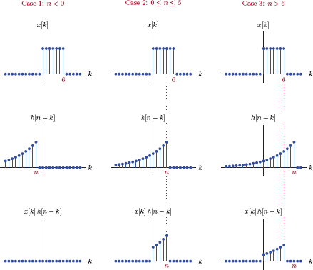
Case 1: n < 0
There is no overlap between the two functions in this case, therefore their product equals zero for all values of k. The output signal is
For this case, the two functions overlap for the range of the index 0 ≤ k ≤ n. Setting summation limits accordingly, the output signal can be written as
The expression in Eqn. (3.139) can be simplified by factoring out the common term (0.9)n and using the geometric series formula (see Appendix C) to yield
Case 3: n > 6
For n > 6 the overlap of the two functions will occur in the range 0 ≤ k ≤ 6, so the summation limits need to be adjusted.
Again factoring out the (0.9)n term and using the geometric series formula we get
Thus, we have computed the output signal in each of the three distinct intervals we have identified. Putting these three partial solutions together, the complete solution for the output signal is obtained as
and is shown in Fig. 3.31.

Software resources:
ex_3_21.m
Interactive Demo: conv_demo5.m
The demo program “conv_demo5.m” is based on the discrete-time convolution problem in Example 3.21. It facilitates visualization of the overlapping samples between the functions x[k] and h [n − k] as the index k is varied. The impulse response used in the demo program is in the general form
and can be made identical to the impulse response used in Example 3.21 by setting a = 0.9.
Software resources:
conv_demo5.m
See MATLAB Exercise 3.8. |
3.8 Causality in Discrete-Time Systems
Causality is an important feature of physically realizable systems. A system is said to be causal if the current value of the output signal depends only on current and past values of the input signal, but not on its future values. For example, a discrete-time system defined by the relationship
is causal, and one defined by
is non-causal. Causal systems can be implemented in real-time processing mode where a sample of the output signal is computed in response to each incoming sample of the input signal. On the order hand, implementation of non-causal systems may only be possible in post processing mode where the entire input signal must be observed and recorded before processing can begin.
In the case of a DTLTI system, the causality property can easily be related to the impulse response. Recall that the output signal y[n] of a DTLTI system can be computed as the convolution of its input signal x[n] with its impulse response h[n] as
For the system under consideration to be causal, the computation of y[n] should not require any future samples of the input signal. Thus, the term xn − k] in the summation should not contain index values in the future. This requires
The product h[k]x[n − k] should not have any non-zero values for k < 0. Therefore, the impulse response h[n] should be equal to zero for all negative index values:
For a causal DTLTI system, the convolution relationship in Eqn. (3.146) can be written in the right-sided form by setting the lower limit of the summation index equal to zero:
3.9 Stability in Discrete-Time Systems
A system is said to be stable in the bounded-input bounded-output (BIBO) sense if any bounded input signal is guaranteed to produce a bounded output signal.
A discrete-time input signal x[n] is said to be bounded if an upper bound Bx exists such that
for all values of the integer index n. A discrete-time system is stable if a finite upper bound By exists for the output signal in response to any input signal bounded as described in Eqn. (3.150).
For stability of a discrete-time system:
If the system under consideration is DTLTI, it is possible to relate the stability condition given by Eqn. (3.151) to the impulse response of the system as well as its difference equation. Derivation of the necessary condition follows:
The output signal of a DTLTI system is found from its input signal and impulse response through the use of the convolution sum expressed as
The absolute value of the output signal is
Absolute value of a sum is less than or equal to the sum of the absolute values, so an inequality involving y[n] can be written as
The summation term in Eqn. (3.154) can be expressed as
and the inequality in Eqn. (3.154) becomes
Replacing the term |x[n − k]| in Eqn. (3.156) with Bx makes the term on the right side of the inequality even greater, so we have
or, by factoring out the common factor Bx
Eqn. (3.158) leads us to the conclusion
For a DTLTI system to be stable, its impulse response must be absolute summable.
Example 3.22: Stability of a length-2 moving-average filter
Comment on the stability of the length-2 moving-average filter described by the difference equation
Solution: We will approach this problem in two different ways. First, let’s check directly to see if any arbitrary bounded input signal is guaranteed to produce a bounded output signal. The absolute value of the output signal is
Since absolute value of a sum is less than or equal to sum of absolute values, we can derive the following inequality from Eqn. (3.160):
Furthermore, since we assume |x[n]| < Bx for all n, replacing |x[n]| and |x[n − 1]| terms on the right side of the inequality in Eqn. (3.161) does not affect the validity of the inequality, so we have
proving that the output signal y[n] is bounded as long as the input signal x[n] is.
An alternative way to attack the problem would be to check the impulse response for the absolute summability condition in Eqn. (3.159). The impulse response of the length-2 moving-average filter is
which is clearly summable in an absolute sense.
Example 3.23: Stability of the loan balance system
Comment on the stability of the loan balance system discussed in Example 3.7.
Solution: Recall that the governing difference equation is
where c is a positive constant interest rate. This system can be analyzed in terms of its stability using the same approach that we have used in the previous example. However, we will take a more practical approach and analyze the system from a layperson’s perspective.
What if we borrowed the money and never made a payment? The loan balance would keep growing each period. If the initial value of the output signal is y[0] = A and if x[n] = 0 for n ≥ 1, then we would have
which indicates that the system is unstable since we were able to find at least one bounded input signal that leads to an unbounded output signal.
It is also worth noting that the characteristic equation is
and its only solution is at z1 = 1 + c.
The stability of a DTLTI system can also be associated with the modes of the difference equation that governs its behavior. We have seen in Section 3.5.1 that, for a causal DTLTI system, real and complex roots zk of the characteristic polynomial for which |zk| ≥ 1 are associated with unstable behavior. Thus, for a causal DTLTI system to be stable, the magnitudes of all roots of the characteristic polynomial must be less than unity. If a circle is drawn on the complex plane with its center at the origin and its radius equal to unity, all roots of the characteristic polynomial must lie inside the circle for the corresponding causal DTLTI system to be stable.
A side note: In describing the associations between the roots of the characteristic polynomial and stability, we referred to a causal DTLTI system. If we were to consider an anti-causal system, the impulse response of which proceeds in the negative direction toward n → −∞, then the associations described above would have to be reversed. In that case roots outside the unit circle of the complex plane would lead to stable behavior.
Why is stability important for a DTLTI system?
An unstable DTLTI system is one that is capable of producing an unbounded output signal in response to at least some bounded input signals. What is the practical significance of this? Since we are dealing with numerical algorithms implemented via software on a computer, an unstable algorithm may lead to an output signal containing numbers that keep growing until they reach magnitudes that can no longer be handled by the number representation conventions of the processor or the operating system. When this occurs, the software that implements the system ceases to function in the proper way.
3.10 Further Reading
[1] S. Elaydi. An Introduction to Difference Equations. Springer Undergraduate Texts in Mathematics and Technology. Springer, 2005.
[2] W.G. Kelley and A.C. Peterson.Difference Equations: An Introduction With Applications. Harcourt/Academic Press, 2001.
[3] V. Lakshmikantham. Theory of Difference Equations Numerical Methods and Applications. Marcel Dekker, 2002.
[4] R.E. Mickens. Difference Equations: Theory and Applications. Van Nostrand Reinhold Company, 1990.
MATLAB Exercises
MATLAB Exercise 3.1: Writing functions for moving average filters
In this exercise we will develop MATLAB functions for implementing the length-2 and length-4 moving average filters that were discussed in Examples 3.4 and 3.5 respectively. As stated before, our purpose is not the development of fastest and most efficient functions. MATLAB already includes some very powerful functions for implementing a wide variety of discrete-time systems, and those could certainly be used for the simulation of moving average filters as well. The use of two of these built-in MATLAB functions, namely conv(..) and filter(..), will be illustrated in later exercises. In this exercise, our purpose in developing our own functions for simulating moving average filters is to provide further insight into their operation. Therefore, we will sacrifice execution speed and efficiency in favor of a better understanding of coding a difference equation for a moving average filter.
Before developing any MATLAB function, it would be a good idea to consider how that function would eventually be used. Our development of the MATLAB code in this exercise will parallel the idea of real-time processing where the input and the output signals exist in the form of ”data streams” of unspecified length. Algorithmically, the following steps will be executed:
- Pick the current input sample from the input stream.
- Process the current input sample through the moving average filter to compute the current output sample.
- Put the current output sample into the output stream.
- Repeat steps 1 through 3.
Let us begin by developing a function named "ss movavg2" to implement step 2 above for a length-2 moving average filter. The function will be used with the syntax
y = ss_movavg2(x)
where "x" represents the current input sample, and "y" is the current output sample. Once developed, the function can be placed into the loop described above to simulate a length-2 moving average filter with any input data stream.
The difference equation of a length-2 moving average filter is
A local variable named "xnm1" will be used for keeping track of the previous sample x[n−1]. The following two lines would compute the output sample and update the previous input sample for future use.
y = (x+ xnm1)/2;
xnm1 = x;
Herein lies our first challenge: In MATLAB, local variables created within functions are discarded when the function returns. The next time the same function is called, its local variable "xnm1" would not have the value previously placed in it. The solution is to declare the variable "xnm1" to be a persistent variable, that is, a variable that retains its value between function calls. Following is a listing of the completed function ss_movavg2(..):
1 function y=ss_movavg2 (x)
2 persistent xnm1;
3 if isempty (xnm1)
4 xnm1 = 0;
5 end ;
6 y = (x+xnm1)/2;
7 xnm1 = x;
Another detail is that the first time a persistent variable is created (the first time the function ss_movavg2(..) is called), it is created as an empty matrix. Lines 3 through 5 of the code above set the variable "xnm1" equal to zero if it happens to be empty.
The function ss_movavg4(..) can be developed in a similar manner. Consider Eqn. (3.13). In addition to x[n − 1] we also need to keep track of two input samples prior to that, namely x[n − 2] and x[n − 3]. Therefore we will define two additional local variables with the names "xnm2" and "xnm3", and declare them to be persistent as well. The code for the function ss_movavg4(..) is listed below.
1 function y = ss_movavg4(x)
2 persistent xnm1 xnm2 xnm3;
3 if isempty (xnm1)
4 xnm1 = 0;
5 end;
6 if isempty (xnm2)
7 xnm2 = 0;
8 end;
9 if isempty (xnm3)
10 xnm3 = 0;
11 end;
12 y = (x+ xnm1 + xnm2 + xnm3)/4;
13 xnm3 = xnm2;
14 xnm2 = xnm1;
15 xnm1 = x;
In lines 13 through 15 of the code we perform bookkeeping, and prepare the three local variables for the next call to the function. The value x[n] we have now will be the ”previous sample” x[n − 1] the next time this function is called, and similar logic applies to the other two variables as well. Therefore the values of {“x”, “xnm1”, and “xnm2”} need to be moved into {“xnm1”, “xnm2”, and “xnm3”} respectively. In doing this, the order of assignments is critical. Had we used the order
13 xnm1 = x;
14 xnm2 = xnm1;
15 xnm3 = xnm2;
all three variables would have ended up (incorrectly) with the same value.
A final detail regarding persistent variables is that sometimes we may need to clear them from memory. Suppose we want to use the function ss_movavg2(..) with another data stream, and need to clear any persistent variables left over from a previous simulation. The following command accomplishes that:
>> clear ss_movavg2
ss_movavg2.m
ss_movavg4.m
MATLAB Exercise 3.2: Testing the functions written in MATLAB Exercise 3.1
In this exercise we will develop the code for testing the moving average filtering functions developed in Exercise 3.1. Daily values of the Dow Jones Industrial Average data for the years 2001 through 2003 are available in MATLAB data file “djia.mat”in MATLAB variables “x2001”, “x2002”and “x2003”. The following script computes the length-4 moving average for the 2003 data, and graphs both the input and the output signals.
1 % Script matex_3_2a.m
2 %
3 load 'djia mat'; % Load the input data stream.
4 output = []; % Create an empty output stream.
5 clear ss_movavg4; % Clear persistent variables.
6 nsamp = length(x2003); % Number of samples in the input stream.
7 for n=1: nsamp
8 x = x2003(n); % "x" is the current input sample.
9 y = ss_movavg4(x); % "y" is the current output sample.
10 output = [output,y]; % Append "y" to the output stream.
11 end;
12 % Graph input and output signals.
13 clf;
14 plot ([1: nsamp], x2003,[1: nsamp], output);
15 axis ([1,252,7500,10500]);
Note that the function ss_movavg4(..) begins with its persistent variables “xnm1”, “xnm2”, “xnm3” each set equal to 0. As a result, the first three samples of the output will be inaccurate. This problem can be alleviated by prepending the last three samples of the year 2002 data to the year 2003 data before we begin processing.
The MATLAB script above can be easily modified to simulate a length-2 moving average filter by substituting function ss_movavg2(..) in place of function ss_movavg4(..).
Software resources:
matex_3_2a.m
matex_3_2b.m
djia.mat
MATLAB Exercise 3.3: Writing and testing a function for the exponential smoother
Consider the exponential smoother introduced in Example 3.6 with the difference equation
We will implement the exponential smoother in MATLAB and test it with the Dow Jones Industrial Average data using the same algorithmic approach as in earlier exercises:
- Pick the current input sample from the input stream.
- Process the current input sample through the moving average filter to compute the current output sample.
- Put the current output sample into the output stream.
- Repeat steps 1 through 3.
A function named “ss_expsmoo” will be developed for implementing step 2 of the algorithm. The syntax of the function is
y = ss_expsmoo (x, alpha)
where “x” represents the current input sample, and “y” is the current output sample. The parameter “alpha” belongs to the exponential smoother. A persistent variable named “ynm1” is utilized for keeping track of the previous output sample y[n − 1]. The code for the function ss_expsmoo(..) is listed below:
1 function y = ss_expsmoo(x, alpha)
2 persistent ynm1;
3 if isempty (ynm1)
4 ynm1 = 0;
5 end;
6 y = (1- alpha)* ynm1 + alpha *x;
7 ynm1 = y;
The following script computes the output of the exponential smoother for the 2003 Dow Jones data as input, and graphs both the input and the output signals.
1 % Script : matex_3_3.m
2 %
3 load 'djia.mat'; % Load the input data stream.
4 output = []; % Create an empty output stream.
5 clear ss_expsmoo; % Clear persistent variables.
6 nsamp = length (x2003); % Number of samples in the input stream.
7 alpha = 0.1; % Parameter for exponential smoother.
8 for n =1:nsamp
9 x = x2003(n); % ”x” is the current input sample.
10 y = ss_expsmoo (x, alpha); % ”y” is the current output sample.
11 output = [output,y]; % Append ”y” to the output stream.
12 end;
13 % Graph input and output signals.
14 clf;
15 plot ([1:nsamp], x2003,[1:nsamp], output);
16 axis ([1,252,7500,10500]);
Software resources:
matex_3_3.m
ss_expsmoo.m
MATLAB Exercise 3.4: Iteratively solving a difference equation
It was shown in Section 3.5 that one way to solve a difference equation is to iterate through it one sample index at a time. In this exercise we will explore this concept in MATLAB, using the difference equation for the loan balance problem introduced in Example 3.7. While the specific problem at hand is quite simplistic, it will help us highlight some of the challenges encountered in adapting a signal-system interaction problem for MATLAB coding, in particular with the vector indexing scheme of MATLAB.
The system under consideration accepts monthly payment data x[n] as input and produces an output signal y[n] that represents the balance at the end of each month. The difference equation for the system was given by Eqn. (3.15) and will be repeated here:
Let the amount borrowed be $10,000 which we will place into y[0] as the initial value of the output signal. Let us also assume that $100 will be paid each month starting with month 1. Thus, the input signal would be
Using a monthly interest rate of 0.5 percent, meaning c = 0.5/100 = 0.005, we would like to compute the output signal for n = 1,..., 18. Following statements create two vectors “xvec”and “yvec”:
>> xvec = [0,100*ones(1,18)];
>> yvec = [10000,zeros(1,18)];
The length-19 vector “xvec” contains payment data. Its first element is zero, and all other elements are equal to 100. The vector “yvec” holds samples of the output signal. Its first element is initialized to 10000, the loan amount, and other elements are set equal to zero as place holders to be modified later.
One of the difficulties encountered in representing discrete-time signals with vectors is that MATLAB vectors do not have an element with index 0; the first element of a vector always has an index of 1. When we translate the difference equation of the system into code, we need to remember that
and so on. Fortunately, this is not a difficult problem to overcome. The method we will use in this exercise is not the most elegant, but it is one that will keep us continuously aware of the indexing differences between MATLAB vectors and our signals. The script listed below iterates through the difference equation. Notice how the MATLAB variable “offset”is used in line 9 to deal with the indexing problem.
1 % Script: matex_3_4a.m
2 %
3 xvec = [0,100*ones(1,18)]; % Vector to hold input signal.
4 yvec = [10000,zeros(1,18)]; % Vector to hold output signal.
5 c = 0.005; % Interest rate.
6 offset = 1; % Offset to fix index issues.
7 % Start the loop to compute the output signal.
8 for n =1:18
9 yvec(offset+n)=(1+c)*yvec(offset+n-1)-xvec(offset+n);
10 end;
11 % Display the output signal.
12 tmp = [[0:18]', yvec'];
13 disp (tmp);
The last two lines
12 tmp = [[0:18]', yvec'];
13 disp (tmp);
create a 19 by 2 matrix “tmp” in which the first column contains the indices from 0 to 19, and the second column contains the corresponding sample amplitudes of the output signal. A better looking tabulated display of the results can be produced with the use of the fprintf(..) function. The modified script shown below tabulates the results a bit more cleanly, and also graphs the output signal y[n].
1 % Script: matex_3_4b.m
2 %
3 xvec = [0,100*ones(1,18)]; % Vector to hold input signal.
4 yvec = [10000,zeros(1,18)]; % Vector to hold output signal.
5 c = 0.005; % Interest rate.
6 offset = 1; % Offset to fix index issues.
 7 fprintf (1, 'Index Input Output
'),  % Print header.
8 % Start the loop to compute and print the output signal.
9 for n=1:18
10 yvec(offset+n)=(1+c)* yvec(offset+n-1)-xvec(offset+n);
11 fprintf (1,'%5d %5.2f %5.2 f
',n, xvec(offset+n),yvec(offset+n));
12 end;
13 % Graph the output signal.
14 stem ([0:18], yvec);
Software resources:
matex_3_4a.m
matex_3_4b.m
MATLAB Exercise 3.5: Implementing a discrete-time system from its block diagram
In this exercise we will implement the discrete-time system for which a block diagram was obtained in Example 3.16, Fig. 3.24. A MATLAB function named “sys1” will be developed with the syntax
y = sys1(x)
where “x” represents the current input sample, and “y” is the current output sample. The function sys1(..) is used in a loop structure for processing samples from an input data stream one sample at a time.
Let the outputs w[n − 1], w[n − 2] and w[n − 3] of the three delay elements from left to right be represented by MATLAB variables “wnm1”, “wnm2” and “wnm3” respectively. These are the persistent variables in sys1(..). When the function is first called, the initial values obtained in Example 3.16 are placed into the persistent variables. A listing of the completed function sys1(..) is given below:
1 function y = sys1(x)
2 persistent wnm1 wnm2 wnm3;
3 if isempty(wnm1)
4 wnm1 = 1.0682; % Initial value w[-1]
5 end;
6 if isempty(wnm2)
7 wnm2 = 1.7149; % Initial value w[-2]
8 end;
9 if isempty(wnm3)
10 wnm3 = 0.1674; % Initial value w[-3]
11 end;
12 wn = x+0.7*wnm1+0.8*wnm2-0.84*wnm3; % Eqn. (3.101)
13 y = 0.1*wn+0.2*wnm1+0.3*wnm2; % Eqn. (3.102)
14 % Prepare for the next call to the function.
15 wnm3 = wnm2;
16 wnm2 = wnm1;
17 wnm1 = wn;
The script listed below can be used for testing the function sys1(..) with a unit-step input signal and graphing the resulting output signal.
1 % Script: matex_3_5.m
2 %
3 input = ones (1,50); % Input data stream.
4 output = []; % Create an empty output stream.
5 clear sys1; % Clear persistent variables.
6 nsamp = length(input); % Number of samples in the input stream.
7 for n=1:nsamp
8 x = input (n); % "x" is the current input sample.
9 y = sys1 (x); % "y" is the current output sample.
10 output = [output,y]; % Append "y" to the output stream.
11 end;
12 % Graph the output signal.
13 clf;
14 stem ([0:nsamp-1],output);
15 title ('The output signal'),
16 xlabel ('Index n'),
17 ylabel ('y[n]'),
The graph produced by this script is shown in Fig. 3.32. Compare it to the result displayed in the interactive demo program dgm_demo1.m.
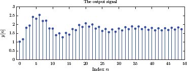
Software resources:
matex_3_5.m
sys1.m
MATLAB Exercise 3.6: Discrete-time system of MATLAB Exercise 3.5 revisited
Consider again the system that was implemented in MATLAB Exercise 3.5. In this exercise we will implement the same system using the function filter(..) that is part of MATLAB. Recall that the system in question was introduced in Example 3.16. Its difference equation is
The unit-step response of the system is to be determined subject to the initial conditions
The function filter(..) implements the difference equation
using a transposed direct-form II implementation which is different than the block diagram used in MATLAB Exercise 3.5. In both Example 3.16 and MATLAB Exercise 3.5 we have converted the initial output values y[−1], y[−2], and y[−3] to values w[−1], w[−2] and w[−3] for the block diagram in Fig. 3.24. This step will need to be revised when using the function filter(..).
The syntax of the function filter(..) is
y = filter(b,a,x,zi)
Meanings of parameters are explained below:
“b”: |
Vector of feed-forward coefficients b0, b1,..., bM |
“a”: |
Vector of feedback coefficients a0, a1,...,aN |
“x”: |
Vector containing samples of the input signal |
“y”: |
Vector containing samples of the output signal |
“zi”: |
Vector containing initial values of the delay elements for the transposed direct-form II block diagram |
The vector “zi” is obtained from the initial values of input and output samples through a call to the function filtic(..). The script listed below computes and graphs the output signal of the system using the two MATLAB functions mentioned. It can easily be verified that the output signal obtained is identical to that of MATLAB Exercise 3.5.
1 % Script : matex_3_6.m
2 %
3 a = [1,-0.7,-0.8,0.84]; % Feedback coefficients.
4 b = [0.1,0.2,0.3]; % Feed - forward coefficients,
5 y_init = [0.5,0.3,-0.4]; % y[-1], y[-2], and y[-3].
6 x_init = [0,0,0]; % x[-1], x[-2], and x[-3].
7 inp = ones(1,50); % Unit - step input signal.
8 zi = filtic(b,a,y_init,x_init);
9 out = filter (b,a,inp,zi);
10 % Graph the output signal.
11 clf;
12 stem([0:49],out);
13 title('The output signal'),
14 xlabel('Index n'),
15 ylabel('y[n]'),
Software resources:
matex_3_6.m
MATLAB Exercise 3.7: Convolution using MATLAB
In Example 3.19 we have discussed the convolution operation applied to two finite-length signals, namely
and
MATLAB has a very convenient function conv(..) for performing the convolution operation on two vectors that hold samples of the signals h[n] and x[n]. The following set of statements create two vectors “h” and “x” corresponding to the signals we are considering, and then compute their convolution:
>> h = [4,3,2,1];
>> x = [-3,7,4];
>> y = conv(h,x)
y =
-12 19 31 23 15 4
The convolution operator is commutative, that is, the roles of h[n] and x[n] can be reversed with no effect on the result. Therefore, the statement
>> y = conv(x,h)
produces exactly the same result.
The MATLAB vector “y” produced by the function conv(..) starts with index 1, a characteristic of all MATLAB vectors. Consequently, an attempt to graph it with a statement like
>> stem(y);
results in the stem graph shown in Fig. 3.33.
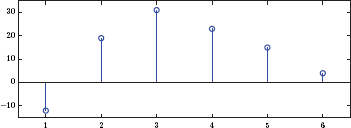
A correctly indexed stem graph can be obtained by the statements
>> n = [0:5];
>> stem(n,y);
and is shown in Fig. 3.34.
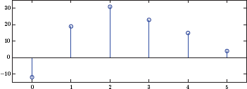
What if the starting indices of the two signals h[n] and x[n] are notat n = 0 but are specified as arbitrary values Nh and Nx respectively? (See Example 3.20.) We could simply adjust the vector “n” to accommodate the change. Instead, we will use this as an opportunity to develop a wrapper function that utilizes the built-in conv(..) function of MATLAB, but also automates the process of generating the appropriate index vector “n” to go with it. The listing for the function ss_conv(..) is given below:
1 function [y,n] = ss_conv(h,x,Nh,Nx)
2 y = conv (h,x);
3 Ny = length(y); % Number of samples in y[n].
4 nfirst = Nh+Nx; % Correct index for the first sample
5 % in vector "y".
6 nlast = nfirst+Ny-1; % Correct index for the last sample
7 % in vector "y".
8 n = [nfirst:nlast];
Parameters “Nh” and “Nx” are the correct indices that should be associated with the first samples of vectors “h” and “x” respectively. Example usage of the function ss_conv(..) is given below:
>> [y,n] = ss_conv(h,x,5,7)
>> stem(n,y);
Software resources:
matex_3_7.m
ss_conv.m
MATLAB Exercise 3.8: Implementing a moving average filter through convolution
Consider again the problem of applying a moving-average filter to a signal for the purpose of producing a smoother version of it at the filter output. Suppose the signal x[n] contains samples of the Dow Jones Industrial average data for the calendar year 2003, and we would like to apply a length-50 moving-average filter to it. While it is possible to write a function to implement a length-50 moving-average filter in a way similar to the development of the functions ss_movavg2(..) and ss_movavg4(..) in MATLAB Exercise 3.1, that would be greatly impractical due to the fact that we need to perform bookkeeping on 49 prior input samples at any given time. Instead, we will solve the problem using convolution.
The impulse response of the length-50 moving-average filter is
which can be represented with a MATLAB vector obtained with the statement
>> h = 1/50*ones (1,50);
The following set of statements statements load the MATLAB data file “djia.mat”into memory, and list the contents of MATLAB workspace so far.
>> load 'djia. mat';
>> whos
Name Size Bytes Class Attributes
h 1x50 400 double
x2001 1x248 1984 double
x2002 1x252 2016 double
x2003 1x252 2016 double
We are assuming that we have started a fresh session for this exercise; otherwise there may be additional variables listed above. The data for the calendar year is in vector “x2003”, and has 252 samples. Thus, we have an input signal x[n] for n = 0,...,251. Its convolution with the impulse response in vector “h” can be obtained with the statements
>> x = x2003;
>> y2003 = conv (h,x);
There is one practical problem with this result. Recall the discussion in Example 3.3 about observing the input signal through a window that holds as many samples as the length of the filter, and averaging the window contents to obtain the output signal. For the first 49 samples of the output signal, the window is only partially full. (Refer to Fig. 3.6.) In the computation of y[0], the only meaningful sample in the window is x[0], and all samples to the left of it are zero-valued. The next output sample y[n] will be based on averaging two meaningful samples x[1] and x[0] along with 48 zero-amplitude samples, and so on. As a result, the first meaningful sample of the output signal (meaningful in the sense of a moving average) will occur at index n = 49 when, for the first time, the window is full.
To circumvent this problem and obtain meaningful moving-average values for all 2003 data, we will prepend the signal x[n] with an additional set of 49 samples borrowed from the last part of the data for calendar year 2002. The following MATLAB statement accomplishes that:
>> x = [x2002(204:252),x2003];
The resulting vector “x” represents the signal x[n] that starts with index n = −49. We can now convolve this signal with the impulse response of the length-50 moving-average filter to obtain the output signal y[n] which will also begin at index n = −49. The statement
>> y = conv(h,x);
produces a vector “y” with 350 elements. Its first 49 elements correspond to signal samples y[−49] through y[−1], and represent averages computed with incomplete data due to empty slots on the left side of the window. In addition, the last 49 elements of the vector “y” corresponding to signal samples y[252] through y[300] also represent averages computed with incomplete data, in this case with empty slots appearing on the right side of the window. We will obtain the smoothed data for the index range n = 0,...,251 by discarding the first and the last 49 samples of the vector “y”.
>> y = y(50:301);
>> plot([0:251],x2003,':',[0:251],y, '-'),
The resulting graph is shown in Fig. 3.35.

Software resources:
matex_3_8.m
Problems
3.1. A number of discrete-time systems are specified below in terms of their input-output relationships. For each case determine if the system is linear and/or time-invariant.
- y[n] = x[n]u[n]
- y[n] = 3x[n] + 5
- y[n] = 3x[n] + 5u[n]
- y[n] = n x[n]
- y[n] = cos(0.2πn) x[n]
- y[n] = x[n] + 3x[n − 1]
- y[n] = x[n] + 3 x[n − 1]x[n − 2]
3.2. A number of discrete-time systems are described below. For each case determine if the system is linear and/or time-invariant.
3.3. Consider the cascade combination of two systems shown in Fig. P.3.3(a).
Let the input-output relationships of the two subsystems be given as
Write the relationship between x[n] and y[n].
Let the order of the two subsystems be changed as shown in Fig. P.3.3(b). Write the relationship between x[n] and . Does changing the order of two subsystems change the overall input-output relationship of the system?
3.4. Repeat Problem 3.3 with the following sets of subsystems:
3.5. The response of a linear and time-invariant system to the input signal x[n] = δ [n] is given by
Determine the response of the system to the following input signals:
- x[n] = δ[n] + δ [n − 1]
- x[n] = δ[n] − 2δ[n − 1] + δ[n − 2]
- x[n] = u[n] − u[n − 5]
- x[n] = n (u[n] − u[n − 5])
3.6. Consider a system that is known to be linear but not necessarily time-invariant. Its responses to three impulse signals are given below:
For each of the input signals listed below, state whether the response of the system can be determined from the information given. If the response can be determined, find it. If not, explain why it cannot be done.
- x[n] = 5δ[n − 1]
- x[n] = 3δ[n] + 2δ[n − 1]
- x[n] = δ[n] − 2δ[n − 1] + 4δ[n − 2]
- x[n] = u[n] − u[n − 3]
- x[n] = u[n] − u[n − 4]
-
is used as input to a length-2 moving average filter. Determine the response y[n] for n = 0,...,9. Use x[−1] = 0.
3.8. Consider again the signal x[n] specified in Problem 3.7. If it is applied to a length-4 moving average filter, determine the output signal y[n] for n = 0,...,9. Use x[−1] = x[−2] = x[−3] = 0.
3.9. The signal x[n] specified in Problem 3.7 is used as input to an exponential smoother with α = 0.2. The initial value of the output signal is y[−1] = 1. Determine y[n] for n = 0,...,9.
3.10. Consider the difference equation model for the loan payment system explored in Example 3.7. The balance at the end of month-n is given by
where c is the monthly interest rate and x[n] represents the payment made in month-n. Let the borrowed amount be $10,000 to be paid back at the rate of $250 per month and with a monthly interest rate of 0.5 percent, that is, c = 0.005. Determine the monthly balance for n = 1,...,12 by iteratively solving the difference equation.
Hint: Start with the initial balance of y[0] = 10000 and model the payments with the input signal
3.11. Refer to Example 3.9 in which a nonlinear difference equation was found for computing a root of a function. The idea was adapted to the computation of the square root of a positive number A by searching for a root of the function
By iteratively solving the difference equation given by Eqn. (3.25), approximate the square root of
- A = 5
- A = 17
- A = 132
In each case carry out the iterations until the result is accurate up to the fourth digit after the decimal point.
3.12. For each homogeneous difference equation given below, find the characteristic equation and show that it only has simple real roots. Find the homogeneous solution for n ≥ 0 in each case subject to the initial conditions specified.
Hint: For part (e) use MATLAB function roots(..) to find the roots of the characteristic polynomial.
3.13. For each homogeneous difference equation given below, find the characteristic equation and show that at least some of its roots are complex. Find the homogeneous solution for n ≥ 0 in each case subject to the initial conditions specified.
Hint: For part (d) use MATLAB function roots(..) to find the roots of the characteristic polynomial.
3.14. For each homogeneous difference equation given below, find the characteristic equation and show that it has multiple-order roots. Find the homogeneous solution for n ≥ 0 in each case subject to the initial conditions specified.
Hint: For parts (c) and (d) use MATLAB function roots(..) to find the roots of the characteristic polynomial.
3.15. Solve each difference equation given below for the specified input signal and initial conditions. Use the general solution technique outlined in Section 3.5.2.
3.16. Consider the exponential smoother explored in Examples 3.6 and 3.14. It is modeled with the difference equation
Let y[−1] = 0 so that the system is linear.
- Let the input signal be a unit step, that is, x[n] = u[n]. Determine the response of the linear exponential smoother as a function of α.
- Let the input signal be a unit ramp, that is, x[n] = n u[n]. Determine the response of the linear exponential smoother as a function of α.
3.17. Consider a first-order differential equation in the form
The derivative can be approximated using the backward difference
where T is the step size.
Using the approximation for the derivative in the differential equation, express ya (t) in terms of ya (t − T) and xa (t).
Convert the differential equation to a difference equation by defining discrete-time signals
Show that the resulting difference equation corresponds to an exponential smoother. Determine its parameter α in terms of A and T.
3.18. Construct a block diagram for each difference equation given below.
- y[n] + 0.2y[n − 1] − 0.63y[n − 2] = x[n] + x[n − 2]
- y[n]− 2.5y[n − 1] + 2.44y[n − 2]− 0.9y[n − 3] = x[n] − 3x[n − 1] + 2x[n − 2]
- y[n]− 0.49y[n − 2] = x[n]− x [n − 1]
- y[n] + 0.6y[n − 1]− 0.51y[n − 2]− 0.28y[n − 3] = x[n] − 2x[n − 2]
3.19. Two DTLTI systems with impulse responses h1[n] and h2[n] are connected in cascade as shown in Fig. P.3.19(a).
Determine the impulse response heq[n] of the equivalent system, as shown in Fig. P.3.19(b) in terms of h1[n] and h2[n].
Hint: Use convolution to express w[n] interms of x[n]. Afterwards use convolution again to express y[n] in terms of w[n].
Let h1[n] = h2[n] = u [n] − u[n − 5]. Determine and sketch heq[n] for the equivalent system.
With h1[n] and h2[n] as specified in part (b), let the input signal be a unit step, that is, x[n] = u [n]. Determine and sketch the signals w [n] and y[n].
3.20. Two DTLTI systems with impulse responses h1[n] and h2[n] are connected in parallel as shown in Fig. P.3.20(a).
Determine the impulse response heq[n] of the equivalent system, as shown in Fig. P.3.20(b) in terms of h1[n] and h2[n].
Hint: Use convolution to express the signals y1[n] and y2[n] in terms of x[n]. Afterwards express y[n] in terms of y1[n] and y2[n].
Let h1[n] = (0.9)n u[n] and h2[n] = (−0.7)n u[n]. Determine and sketch heq[n] for the equivalent system.
With h1[n] and h2[n] as specified in part (b), let the input signal be a unit step, that is, x[n] = u[n]. Determine and sketch the signals y1[n], y2[n] and y[n].
3.21. Three DTLTI systems with impulse responses h1[n], h2[n] and h3[n] are connected as shown in Fig. P.3.21(a).
- Determine the impulse response heq[n] of the equivalent system, as shown in Fig. P.3.21(b) in terms of h1[n], h2[n] and h3[n].
- Let h1[n] = e−0.1n u[n], h2[n] = δ[n − 2], and h3[n] = e−0.2n u[n]. Determine and sketch heq[n] for the equivalent system.
- With h1[n], h2[n] and h3[n] as specified in part (b), let the input signal be a unit step, that is, x[n] = u[n]. Determine and sketch the signals w[n], y1[n], y2[n] and y[n].
3.22. Consider the DTLTI system shown in Fig. P.3.22(a).
Express the impulse response of the system as a function of the impulse responses of the subsystems.
Let
and
Determine the impulse response heq[n] of the equivalent system.
- Let the input signal be a unit-step, that is, x[n] = u[n]. Determine and sketch the signals w [n], y1[n], y3[n] and y4[n].
3.23. Consider two finite-length signals x[n] and h[n] that are equal to zero outside the intervals indicated below:
In other words, significant samples of x[n] are in the index range Nx1,...,Nx2, and the significant samples of h[n] are in the index range Nh1,...,Nh2.
Let y[n] be the convolution of x[n] and h[n]. Starting with the convolution sum given by Eqn. (3.128), determine the index range of significant samples Ny1,...,Ny2 for y[n].
3.24. Let y[n] be the convolution of two discrete-time signals x[n] and h [n], that is
Show that time shifting either x[n] or h [n] by m samples causes the y[n] to be time shifted by m samples also. Mathematically prove that
and
3.25. Determine the impulse response of each system described below. Afterwards determine whether the system is causal and/or stable.

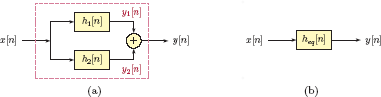


MATLAB Problems
3.26. Refer to the homogeneous difference equations in Problem 3.12. For each one, develop a MATLAB script to iteratively solve it for n = 0,..., 19 using the initial conditions specified. Compare the results of iterative solutions to the results obtained analytically in Problem 3.12.
3.27. Refer to Problem 3.3. The cascade combination of the two subsystems will be tested using the input signal
Write a script to do the following:
- Create an anonymous anonymous function “x” to compute the input signal at all index values specified in a vector “n”.
- Implement the cascade system as shown in Fig. P.3.3(a). Compute the signals w[n] and y[n] for n = 0,..., 29.
- Implement the cascade system in the alternative form shown in Fig. P.3.3(b). Compute the signals and for n = 0,..., 29. Compare y[n] and .
3.28. Repeat the steps of Problem 3.27 using the subsystems described in Problem 3.4.
3.29. Refer to Problem 3.1. Linearity and time invariance of the systems listed will be tested using the two input signals
and
Develop a script to do the following:
Express the two input signals by means of two anonymous functions “x1”and “x2”. Each anonymous function should take a single argument “n” which could either be a scalar or a vector of index values.
Express each of the systems described in Problem 3.1 as an anonymous function. Name the anonymous functions “sys1” through “sys5”. Each should take two arguments “n”and “x”.
Compute the response of each system to
Identify which systems fail the linearity test.
Compute the response of each system to
Identify which systems fail the time-invariance test.
-
Develop a function ss_lbal(..) to iteratively solve the loan balance difference equation explored in Problem 3.10. It should have the following interface:
bal = ss_lbal(A,B,c,n)The arguments are:
A:
Amount of the loan; this is also the balance at n = 0
B:
Monthly payment amount
c:
Monthly interest rate
n:
Index of the month in which the balance is sought
bal:
Computed balance after n months
Write a script to test the function with the values specified in Problem 3.10.
3.31. Refer to Problem 3.11.
Develop a MATLAB function ss_sqrt(..) that iteratively solves the nonlinear difference equation given by Eqn. (3.25) to approximate the square root of a positive number A. The syntax of the function should be
y = ss_sqrt(A,y_init,tol)The argument “A” represents the positive number the square root of which is being sought, “y init” is the initial value y[−1], and “tol” is the tolerance limit ∊. The function should return when the difference between two consecutive output samples is less than the tolerance limit, that is,
Write a script to test the function ss_sqrt(..) with the values A = 5, A = 17 and A = 132.
3.32. Refer to Problem 3.16 in which the response of the linear exponential smoother to unit-step and unit-ramp signals were found as functions of the parameter α. Consider the input signal shown in Fig. P.3.32.
Develop a script to do the following:
- Create an anonymous function yu(..) to compute the unit-step response of the linear exponential smoother. It should take two arguments, “alpha”and “n”, and should return the unit-step response evaluated at each index in the vector “n”.
- Create an anonymous function yr(..) to compute the unit-ramp response of the linear exponential smoother. Like the function yu(..), the function yr(..) should also take two arguments, “alpha”and “n”, and should return the unit-ramp response evaluated at each index in the vector “n”.
- Express the input signal x[n] using a combination of scaled and time shifted unit-step and unit-ramp functions.
- Use the anonymous functions yu(..) and yr(..) to compute and graph the output signal y[n]. Try with α = 0.1, 0.2, 0.3 and compare.

MATLAB Projects
3.33. Consider the logistic growth model explored in Example 3.8. The normalized value of the population at index n is modeled using the nonlinear difference equation
where r is the growth rate. This is an example of a chaotic system. Our goal in this project is to simulate the behavior of a system modeled by the nonlinear difference equation given, and to determine the dependency of the population growth on the initial value y[0] and the growth rate r.
Develop a function called ss_lgrowth(..) with the syntax
y = ss_lgrowth(y_init,r,N)where “y_init” is the initial value of the population at n = 0, “r” is the growth rate, and “N” is the number of iterations to be carried out. The vector returned by the function should have the values
- Write a script to compute y[n] for n = 1,..., 30 with specified values y[0] and r.
- With the growth rate set at r = 1.5, compute and graph y[n] for the cases of y[0] = 0.1, y[0] = 0.3, y[0] = 0.5, y[0] = 0.7. Does the population reach equilibrium? Comment on the dependency of the population at equilibrium on the initial value y[0].
- Repeat the experiment with r =2, 2.5, 2.75, 3. For each value of r compute and graph y[n] for the cases of y[0] = 0.1, y[0] = 0.3, y[0] = 0.5, y[0] = 0.7. Does the population still reach equilibrium? You should find that beyond a certain value of r population behavior should become oscillatory. What is the critical value of r?
3.34. Consider the second-order homogeneous difference equation
with initial conditions y[−1] = p1 and y[−2] = p2. The coefficients a1 and a2 of the difference equation and the initial values p1 and p2 are all real-valued, and will be left as parameters.
Let z1 and z2 be the roots of the characteristic polynomial. On paper, solve the homogeneous difference equation for the three possibilities for the roots:
- The roots are real and distinct.
- The roots are a complex conjugate pair.
- The two roots are real and equal.
Find the solution y[n] as a function of the roots z1 and z2 as well as the initial values p1 and p2.
Develop a MATLAB function ss_de2solve(..) with the syntax
y = ss_de2solve(a1,a2,p1,p2,n)The vector “n” contains the index values for which the solution should be computed. The returned vector “y” holds the solution at the index values in vector “n”so that the solution can be graphed with
stem(n,y)Your function should perform the following steps:
- Form the characteristic polynomial and find its roots.
- Determine which of the three categories the roots fit (simple real roots, complex conjugate pair or multiple roots).
- Compute the solution accordingly.
Test the function ss_de2solve(..) with the homogeneous difference equations in Problems 3.12a, b, c, d, Problems 3.13a, b, c, and Problem 3.14a and b.
3.35. One method of numerically approximating the integral of a function is the trapezoidal integration method. Consider the function xa (t) as shown in Fig. P.3.35.
The area under the function from t = (n − 1)T to t = nT may be approximated with the area of the shaded trapezoid:
Let
It follows that
If we define discrete-time signals x[n] and y[n] as
then y[n − 1] = ya(nT − T), and we obtain the difference equation
which is the basis of a trapezoidal integrator.
Develop a function ss_integ(..) with the following interface:
val = ss_integ(xa,lim1,lim2,y_init,k)The arguments are:
xa:
Handle to an anonymous function for xa (t)
lim1:
Lower limit of the integral
lim2:
Upper limit of the integral
y_init:
Initial value of the integral
k:
Number of time steps from lim1 to lim2
val:
Trapezoidal approximation to the integral
Write a script to test the function with the integrand
and compare its approximate integral with the correct result given by
Hint: Set the lower limit of the integral to t = 0.

1 cos (a + b) = cos(a) cos(b) − sin (a) sin(b).
2 cos (a + b) = cos(a) cos(b) − sin (a) sin(b) and sin (a + b) = sin(a) cos(b) + cos(a) sin(b).