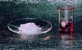
FIGURE 1.3 Physical appearance of ionic liquids. On the left is methyl-tri-n-butylammonium dioctyl sulfosuccinate with a melting point around 313 K. On the right is 1-butyl-3-methyl imidazolium (diethylene glycol monomethyl ether) sulfate which is liquid at room temperature [69].

FIGURE 1.4 A room temperature ionic liquid compared with common table salt [47].

FIGURE 1.5 Metal-based ionic liquids exhibit a wide range of colors. The liquids are from left to right: copper-based compound, cobalt-based compound, manganese-based compound, iron-based compound, nickel-based compound, and vanadium-based compound [84]. Source: Courtesy of Sandia National Laboratories, Albuquerque, NM.

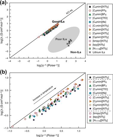
FIGURE 1.12 Walden plot of log (molar conductivity, Λ) against log (reciprocal viscosity η⁻¹) for ionic liquids. The upper figure (a) includes a classification of good and poor ionic liquids, as well as nonionic liquids [14]. The lower figure (b) is a close-up view of the region occupied by typical aprotic ionic liquids. The solid line indicates the ideal line for a completely dissociated strong electrolyte aqueous solution (KCl aq.) [221].

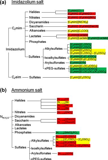
FIGURE 1.15 Proposed dendrograms to represent the toxicities of selected (a) imidazolium and (b) ammonium ionic liquids [276,282].

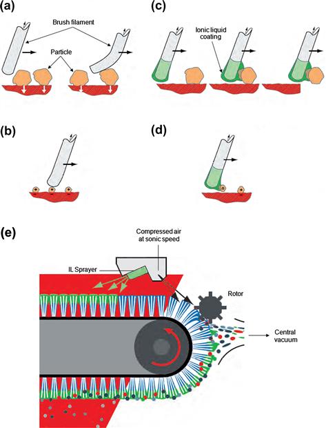
FIGURE 1.17 The removal of contaminant particles by brush cleaning (a and b) is much more efficient if the brush filaments are coated with a conducting ionic liquid film, applied by a spray from a fine nozzle (c, d and e). The adhering particles are removed by a rotor at the end of the process [334,335]. Source: Courtesy of IoLiTec GmbH and Wandres Micro-Cleaning, Germany.

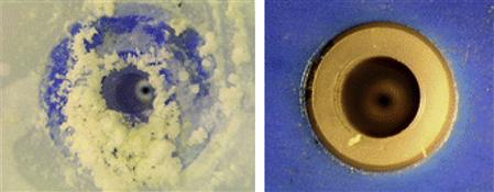
FIGURE 1.18 A spray nozzle for aqueous solutions of sodium chloride (left) and a hydrophilic ionic liquid (right), each after 10 h of operation [334]. Source: Courtesy of IoLiTec GmbH, Germany.

FIGURE 3.1 Cleaning process window depicting particle adhesion force distribution (left) compared with structural integrity force (right) with optimized cleaning forces located in between.

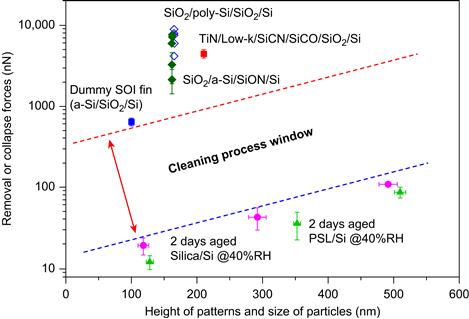
FIGURE 3.5 Cleaning process window showing less energy required to remove particles vs damage structures. Figure provided courtesy of Tae-Gon Kim and used with permission.

FIGURE 3.13 Droplet size and velocity distribution from atomized liquid spray with gas flow rate of 25 L/min. Reproduced by permission of ECS - The Electrochemical Society.

FIGURE 3.19 Damage to photoresist structures for two droplet sizes at varying velocity.

FIGURE 3.20 Correlation of droplet energy density with number of damage sites.

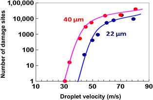
FIGURE 3.25 Threshold curves for particle removal and pattern damage generation with dual-fluid Nanospray2 and NanosprayÅ nozzles.

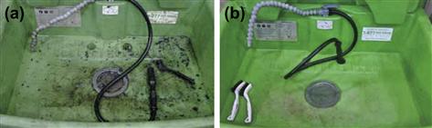
FIGURE 4.4 Parts cleaner sink (a) prior to cleaning, and (b) after cleaning [30]. Source: Courtesy of J. Walter Co. Ltd.

FIGURE 4.5 Photos of a truck fueling bay before (a) and after (b) microbial cleaning [36]. Source: Courtesy Worldware Enterprises, Canada.

FIGURE 4.6 A cleaning tank (a) after drainage but before cleaning, and (b) after microbial treatment [34]. Source: Courtesy of J. Walter Co. Ltd.

FIGURE 4.8 Effect of biocleaning with Pseudomonas stutzeri bacterial strain on the Stories of the Holy Fathers fresco before (a) and after (b) treatment [97].

FIGURE 5.15 The use of a 3D SRO to evaluate the results obtained by four operators (DP, DW, EN, and EN-repeat) using four contact angle measurement procedures (Circle, DSA, Ellipse, and Snake). The horizontal reference lines in each chart are the 95% upper confidence limit (UCL), the mean of all measurements in the study (X), the 95% lower confidence limit (LCL), and the mean of all ranges in the study (R).

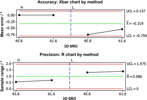
FIGURE 5.16 The half-angle method (H) was used to determine the accuracy and precision of the Langmuir method (L) against two 3D SROs (45.8° and 61.6°). The horizontal reference lines in each chart are the upper 95% confidence limit (UCL), the mean of all measurements in the study (X), the lower 95% confidence limit (LCL), and the mean of all ranges in the study (R).