
OpenGL ES: Going 3D
Super Jumper worked out rather well with the 2D OpenGL ES rendering engine. Now it’s time to go full 3D. We actually already worked in a 3D space when we defined our view frustum and the vertices of our sprites. In the latter case, the z coordinate of each vertex was simply set to 0 by default. The difference from 2D rendering really isn’t all that big:
- Vertices have not only x and y coordinates, but also a z coordinate.
- Instead of an orthographic projection, a perspective projection is used. Objects further away from the camera appear smaller.
- Transformations, such as rotations, translations, and scales, have more degrees of freedom in 3D. Instead of just moving the vertices in the x-y plane, we can now move them around freely on all three axes.
- We can define a camera with an arbitrary position and orientation in 3D space.
- The order in which we render the triangles of our objects is now important. Objects further away from the camera must be overlapped by objects that are closer to the camera.
The best thing is that we have already laid the groundwork for all of this in our framework. To go 3D, we just need to adjust a couple of classes slightly.
Before We Begin
As in previous chapters, we’ll write a couple of examples in this chapter. We’ll follow the same route as before by having a starter activity showing a list of examples. We’ll reuse the entire framework created over the previous three chapters, including the GLGame, GLScreen, Texture, and Vertices classes.
The starter activity of this chapter is called GL3DBasicsStarter. We can reuse the code of the GLBasicsStarter activity from Chapter 7 and just change the package name for the example classes that we are going to run to com.badlogic.androidgames.gl3d. We also have to add each of the tests to the manifest in the form of <activity> elements again. All our tests will be run in fixed landscape orientation, which we will specify per <activity> element.
Each of the tests is an instance of the GLGame abstract class, and the actual test logic is implemented in the form of a GLScreen instance contained in the GLGame implementation of the test, as seen in Chapter 9. We will present only the relevant portions of the GLScreen instance, to conserve some pages. The naming conventions are again XXXTest and XXXScreen for the GLGame and GLScreen implementation of each test.
Vertices in 3D
In Chapter 7, you learned that a vertex has a few attributes:
- Position
- Color (optional)
- Texture coordinates (optional)
We created a helper class called Vertices, which handles all the dirty details for us. We limited the vertex positions to have only x and y coordinates. All we need to do to go 3D is modify the Vertices class so that it supports 3D vertex positions.
Vertices3: Storing 3D Positions
Let’s write a new class called Vertices3 to handle 3D vertices based on our original Vertices class. Listing 10-1 shows the code.
Listing 10-1. Vertices3.java, Now with More Coordinates
package com.badlogic.androidgames.framework.gl;

import java.nio.ByteBuffer;
import java.nio.ByteOrder;
import java.nio.IntBuffer;
import java.nio.ShortBuffer;

import javax.microedition.khronos.opengles.GL10;

import com.badlogic.androidgames.framework.impl.GLGraphics;

public class Vertices3 {
    final GLGraphics glGraphics;
    final boolean hasColor;
    final boolean hasTexCoords;
    final int vertexSize;
    final IntBuffer vertices;
    final int [] tmpBuffer;
    final ShortBuffer indices;

    public Vertices3(GLGraphics glGraphics,int maxVertices,int maxIndices,
            boolean hasColor,boolean hasTexCoords) {
        this .glGraphics = glGraphics;
        this .hasColor = hasColor;
        this .hasTexCoords = hasTexCoords;
        this .vertexSize = (3 + (hasColor ? 4 : 0) + (hasTexCoords ? 2 : 0)) * 4;
        this .tmpBuffer =new int [maxVertices * vertexSize / 4];

        ByteBuffer buffer = ByteBuffer.allocateDirect(maxVertices * vertexSize);
        buffer.order(ByteOrder.nativeOrder());
        vertices = buffer.asIntBuffer();

        if (maxIndices > 0) {
            buffer = ByteBuffer.allocateDirect(maxIndices * Short.SIZE/ 8);
            buffer.order(ByteOrder.nativeOrder());
            indices = buffer.asShortBuffer();
        }else {
            indices =null ;
        }
    }

    public void setVertices(float [] vertices,int offset,int length) {
        this .vertices.clear();
        int len = offset + length;
        for (int i = offset, j = 0; i < len; i++, j++)
            tmpBuffer[j] = Float.floatToRawIntBits(vertices[i]);
        this .vertices.put(tmpBuffer, 0, length);
        this .vertices.flip();
    }

    public void setIndices(short [] indices,int offset,int length) {
        this .indices.clear();
        this .indices.put(indices, offset, length);
        this .indices.flip();
    }

    public void bind() {
        GL10 gl = glGraphics.getGL();

        gl.glEnableClientState(GL10.GL_VERTEX_ARRAY);
        vertices.position(0);
        gl.glVertexPointer(3, GL10.GL_FLOAT, vertexSize, vertices);

        if (hasColor) {
            gl.glEnableClientState(GL10.GL_COLOR_ARRAY);
            vertices.position(3);
            gl.glColorPointer(4, GL10.GL_FLOAT, vertexSize, vertices);
        }

        if (hasTexCoords) {
            gl.glEnableClientState(GL10.GL_TEXTURE_COORD_ARRAY);
            vertices.position(hasColor ? 7 : 3);
            gl.glTexCoordPointer(2, GL10.GL_FLOAT, vertexSize, vertices);
        }
    }

    public void draw(int primitiveType,int offset,int numVertices) {
        GL10 gl = glGraphics.getGL();

        if (indices !=null ) {
            indices.position(offset);
            gl.glDrawElements(primitiveType, numVertices,
                    GL10.GL_UNSIGNED_SHORT, indices);
        }else {
            gl.glDrawArrays(primitiveType, offset, numVertices);
        }
    }

    public void unbind() {
        GL10 gl = glGraphics.getGL();
        if (hasTexCoords)
            gl.glDisableClientState(GL10.GL_TEXTURE_COORD_ARRAY);

        if (hasColor)
            gl.glDisableClientState(GL10.GL_COLOR_ARRAY);
    }
}
Everything stays the same compared to Vertices, except for a few small things:
- In the constructor, we calculate vertexSize differently since the vertex position now takes three floats instead of two floats.
- In the bind() method, we tell OpenGL ES that our vertices have three rather than two coordinates in the call to glVertexPointer() (first argument).
- We have to adjust the offsets that we set in the calls to vertices.position() for the optional color and texture coordinate components.
That’s all we need to do. Using the Vertices3 class, we now have to specify the x, y, and z coordinates for each vertex when we call the Vertices3.setVertices() method. Everything else stays the same in terms of usage. We can have per-vertex colors, texture coordinates, indices, and so on.
An Example
Let’s write a simple example called Vertices3Test. We want to draw two triangles, one with z being −3 for each vertex and one with z being −5 for each vertex. We’ll also use per-vertex color. Since we haven’t discussed how to use a perspective projection, we’ll just use an orthographic projection with appropriate near and far clipping planes so that the triangles are in the view frustum (that is, near is 10 and far is −10). Figure 10-1 shows the scene.

Figure 10-1. A red triangle (front) and a green triangle (back) in 3D space
The red triangle is in front of the green triangle. It is possible to say “in front” because the camera is located at the origin looking down the negative z axis by default in OpenGL ES (which actually doesn’t have the notion of a camera). The green triangle is also shifted a little to the right so that we can see a portion of it when viewed from the front. It should be overlapped by the red triangle for the most part. Listing 10-2 shows the code for rendering this scene.
Listing 10-2. Vertices3Test.java; Drawing Two Triangles
package com.badlogic.androidgames.gl3d;

import javax.microedition.khronos.opengles.GL10;

import com.badlogic.androidgames.framework.Game;
import com.badlogic.androidgames.framework.Screen;
import com.badlogic.androidgames.framework.gl.Vertices3;
import com.badlogic.androidgames.framework.impl.GLGame;
import com.badlogic.androidgames.framework.impl.GLScreen;

public class Vertices3Test extends GLGame {

    public Screen getStartScreen() {
        return new Vertices3Screen(this );
    }

    class Vertices3Screen extends GLScreen {
        Vertices3 vertices;

        public Vertices3Screen(Game game) {
            super (game);

            vertices = new Vertices3(glGraphics, 6, 0,true ,false );
            vertices.setVertices(new float [] { −0.5f, -0.5f, -3, 1, 0, 0, 1,
                                                0.5f, -0.5f, -3, 1, 0, 0, 1,
                                                0.0f,  0.5f, -3, 1, 0, 0, 1,
                                                0.0f,  -0.5f, -5, 0, 1, 0, 1,
                                                1.0f,  -0.5f, -5, 0, 1, 0, 1,
                                                0.5f,  0.5f, -5, 0, 1, 0, 1}, 0, 7 * 6);
        }

        @Override
        public void present(float deltaTime) {
            GL10 gl = glGraphics.getGL();
            gl.glClear(GL10.GL_COLOR_BUFFER_BIT);
            gl.glViewport(0, 0, glGraphics.getWidth(), glGraphics.getHeight());
            gl.glMatrixMode(GL10.GL_PROJECTION);
            gl.glLoadIdentity();
            gl.glOrthof(−1, 1, -1, 1, 10, -10);
            gl.glMatrixMode(GL10.GL_MODELVIEW);
            gl.glLoadIdentity();
            vertices.bind();
            vertices.draw(GL10.GL_TRIANGLES, 0, 6);
            vertices.unbind();
        }

        @Override
        public void update(float deltaTime) {
        }

        @Override
        public void pause() {
        }

        @Override
        public void resume() {
        }

        @Override
        public void dispose() {
        }
    }
}
As you can see, this is the complete source file. The following examples will show only the relevant portions of this file, since the rest stays mostly the same, apart from the class names.
We have a Vertices3 member in Vertices3Screen, which we initialize in the constructor. We have six vertices in total, a color per vertex, and no texture coordinates. Since neither triangle shares vertices with the other, we don’t use indexed geometry. This information is passed to the Vertices3 constructor. Next, we set the actual vertices with a call to Vertices3.setVertices(). The first three lines specify the red triangle in the front, and the other three lines specify the green triangle in the back, slightly offset to the right by 0.5 units. The third float on each line is the z coordinate of the respective vertex.
In the present() method, we must first clear the screen and set the viewport, as always. Next, we load an orthographic projection matrix, setting up a view frustum big enough to show our entire scene. Finally, we just render the two triangles contained within the Vertices3 instance. Figure 10-2 shows the output of this program.

Figure 10-2. The two triangles—but something’s wrong
Now that is strange. According to our theory, the red triangle (in the middle) should be in front of the green triangle. The camera is located at the origin looking down the negative z axis, and from Figure 10-1 we can see that the red triangle is closer to the origin than the green triangle. What’s happening here?
OpenGL ES will render the triangles in the order in which we specify them in the Vertices3 instance. Since we specified the red triangle first, it will get drawn first. We could change the order of the triangles to fix this. But what if our camera wasn’t looking down the negative z axis, but instead was looking from behind? We’d again have to sort the triangles before rendering according to their distance from the camera. That can’t be the solution. And it isn’t. We’ll fix this in a minute. Let’s first get rid of this orthographic projection and use a perspective one instead.
A note on coordinate systems: You may notice that, in our examples, we start by looking down the z axis, where if z increases toward us, x increases to the right and y increases up. This is what OpenGL uses as the standard coordinate system. An easy way to remember this system is called the right-hand rule. Begin by pressing the tips of your pinky and ring fingers of your right hand against your right palm. Your thumb represents the x axis, your index finger pointed straight out represents the y axis, and your middle finger pointed toward you represents the z axis. See Figure 10-3 for an example. Just remember this rule and it will eventually come quite naturally to you.
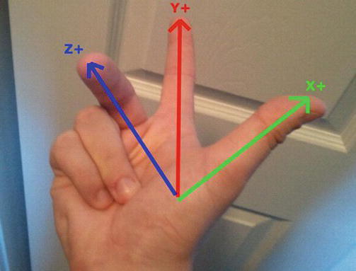
Figure 10-3. The right-hand rule
Perspective Projection: The Closer, the Bigger
Until now, we have always used an orthographic projection, meaning that no matter how far an object is from the near clipping plane, it will always have the same size on the screen. Our eyes show us a different picture of the world. The further away an object is, the smaller it appears to us. This is called perspective projection, which we discussed briefly in Chapter 7.
The difference between an orthographic projection and a perspective projection can be explained by the shape of the view frustum. In an orthographic projection, there is a box. In a perspective projection, there is a pyramid with a cut-off top as the near clipping plane, the pyramid’s base as the far clipping plane, and its sides as the left, right, top, and bottom clipping planes. Figure 10-4 shows a perspective view frustum through which we can view our scene.

Figure 10-4. A perspective view frustum containing the scene (left); the frustum viewed from above (right)
The perspective view frustum is defined by four parameters:
- The distance from the camera to the near clipping plane
- The distance from the camera to the far clipping plane
- The aspect ratio of the viewport, which is embedded in the near clipping plane given by viewport width divided by viewport height
- The field of view, specifying how wide the view frustum is, and therefore, how much of the scene it shows
While we’ve talked about a “camera,” there’s no such concept involved here yet. Just pretend that there is a camera sitting fixed at the origin looking down the negative z axis, as shown in Figure 10-4.
The near and far clipping plane distances are familiar to us from Chapter 7. We just need to set them up so that the complete scene is contained in the view frustum. The field of view is also easily understandable when looking at the right image in Figure 10-4.
The aspect ratio of the viewport is a little less intuitive. Why is it needed? It ensures that our world doesn’t get stretched if the screen to which we render has an aspect ratio that’s not equal to 1.
Previously, we used glOrthof() to specify the orthographic view frustum in the form of a projection matrix. For the perspective view frustum, we could use a method called glFrustumf(). However, there’s an easier way.
Traditionally, OpenGL ES comes with a utility library called GLU. It contains a couple of helper functions for things like setting up projection matrices and implementing camera systems. That library is also available on Android in the form of a class called GLU. It features a few static methods we can invoke without needing a GLU instance. The method in which we are interested is called gluPerspective():
GLU.gluPerspective(GL10 gl, float fieldOfView, float aspectRatio, float near, float far);
This method will multiply the currently active matrix (that is, the projection matrix or the model-view matrix) with a perspective projection matrix, similar to glOrthof(). The first parameter is an instance of GL10, usually the one used for all other OpenGL ES–related business; the second parameter is the field of view, given in angles; the third parameter is the aspect ratio of the viewport; and the last two parameters specify the distance of the near and far clipping planes from the camera position. Since we don’t have a camera yet, those values are given relative to the origin of the world, forcing us to look down the negative z axis, as shown in Figure 10-4. That’s totally fine for our purposes at the moment; we will make sure that all the objects we render stay within this fixed and immovable view frustum. As long as we only use gluPerspective(), we can’t change the position or orientation of our virtual camera. We will always only see a portion of the world when looking down the negative z axis.
Let’s modify Listing 10-2 so that it uses perspective projection. First, just copy over all code from Vertices3Test to a new class called PerspectiveTest, and also rename Vertices3Screen to PerspectiveScreen. The only thing we need to change is the present() method. Listing 10-3 shows the code.
Listing 10-3. Excerpt from PerspectiveTest.java; Perspective Projection
@Override
public void present(float deltaTime) {
    GL10 gl = glGraphics.getGL();
    gl.glClear(GL10.GL_COLOR_BUFFER_BIT);
    gl.glViewport(0, 0, glGraphics.getWidth(), glGraphics.getHeight());
    gl.glMatrixMode(GL10.GL_PROJECTION);
    gl.glLoadIdentity();
    GLU.gluPerspective(gl, 67,
                       glGraphics.getWidth() / (float )glGraphics.getHeight(),
                       0.1f, 10f);
    gl.glMatrixMode(GL10.GL_MODELVIEW);
    gl.glLoadIdentity();
    vertices.bind();
    vertices.draw(GL10.GL_TRIANGLES, 0, 6);
    vertices.unbind();
}
The only difference from the present() method in the previous example is that we are now using GLU.gluPerspective() instead of glOrtho(). We use a field of view of 67 degrees, which is close to the average human field of view. By increasing or decreasing this value, you can see more or less to the left and right. The next thing we specify is the aspect ratio, which is the screen’s width divided by its height. Note that this will be a floating-point number, so we have to cast one of the values to a float before dividing. The final arguments are the near and far clipping plane distances. Given that the virtual camera is located at the origin looking down the negative z axis, anything with a z value less than −0.1 and greater than −10 will be between the near and far clipping planes, and thus be potentially visible. Figure 10-5 shows the output of this example.

Figure 10-5. Perspective (mostly correct)
Now we are actually doing proper 3D graphics. As you can see, there is still a problem with the rendering order of our triangles. That can be fixed by using the almighty z-buffer.
Z-buffer: Bringing Order to Chaos
What is a z-buffer? In Chapter 3 we discussed the framebuffer. It stores the color for each pixel on the screen. When OpenGL ES renders a triangle to the framebuffer, it just changes the color of the pixels that make up that triangle.
The z-buffer is very similar to the framebuffer in that it also has a storage location for each pixel on the screen. Instead of storing colors, it stores depth values. The depth valueof a pixel is roughly the normalized distance of the corresponding point in 3D to the near clipping plane of the view frustum.
OpenGL ES will write a depth value for each pixel of a triangle to the z-buffer by default (if a z-buffer was created alongside the framebuffer). We simply have to tell OpenGL ES to use this information to decide whether a pixel being drawn is closer to the near clipping plane than the pixel that’s currently there. For this, we just need to call glEnable() with an appropriate parameter:
GL10.glEnable(GL10.GL_DEPTH_TEST);
OpenGL ES then compares the incoming pixel depth with the pixel depth that’s already in the z-buffer. If the incoming pixel depth is smaller, its corresponding pixel is closer to the near clipping plane and thus in front of the pixel that’s already in the frame- and z-buffer.
Figure 10-5 illustrates the process. The z-buffer starts off with all values set to infinity (or a very high number). When you render the first triangle, compare each of its pixels’ depth values to the value of the pixel in the z-buffer. If the depth value of a pixel is smaller than the value in the z-buffer, the pixel passes the so-called depth test, or z-test. The pixel’s color will be written to the framebuffer, and its depth will overwrite the corresponding value in the z-buffer. If it fails the test, neither the pixel’s color nor its depth value will be written to the buffers. This is shown in Figure 10-6, where the second triangle is rendered. Some of the pixels have smaller depth values and thus get rendered; other pixels don’t pass the test.

Figure 10-6. Image in the framebuffer (left); z-buffer contents after rendering each of the two triangles (right)
As with the framebuffer, we also have to clear the z-buffer for each frame; otherwise, the depth values from the last frame would still be in there. To do this, we can call glClear(), as per the following:
gl.glClear(GL10.GL_COLOR_BUFFER_BIT | GL10.GL_DEPTH_BUFFER_BIT);
This will clear the framebuffer (or colorbuffer) and the z-buffer (or depthbuffer) all in one go.
Fixing the Previous Example
Let’s fix the previous example’s problems by using the z-buffer. Simply copy all the code over to a new class called ZBufferTest and modify the present() method of the new ZBufferScreen class, as shown in Listing 10-4.
Listing 10-4. Excerpt from ZBufferTest.java; Using the Z-buffer
@Override
public void present(float deltaTime) {
    GL10 gl = glGraphics.getGL();
    gl.glClear(GL10.GL_COLOR_BUFFER_BIT| GL10.GL_DEPTH_BUFFER_BIT);
    gl.glViewport(0, 0, glGraphics.getWidth(), glGraphics.getHeight());
    gl.glMatrixMode(GL10.GL_PROJECTION);
    gl.glLoadIdentity();
    GLU.gluPerspective(gl, 67,
            glGraphics.getWidth() / (float )glGraphics.getHeight(),
            0.1f, 10f);
    gl.glMatrixMode(GL10.GL_MODELVIEW);
    gl.glLoadIdentity();

    gl.glEnable(GL10.GL_DEPTH_TEST);

    vertices.bind();
    vertices.draw(GL10.GL_TRIANGLES, 0, 6);
    vertices.unbind();

    gl.glDisable(GL10.GL_DEPTH_TEST);
}
We first changed the arguments to the call to glClear(). Now both buffers are cleared instead of just the framebuffer.
We also enable depth testing before we render the two triangles. After we are done with rendering all of the 3D geometry, we disable depth testing again. Why? Imagine that we want to render 2D UI elements on top of our 3D scene, such as the current score or buttons. Since we’d use the SpriteBatcher for this, which only works in 2D, we wouldn’t have any meaningful z coordinates for the vertices of the 2D elements. We wouldn’t need depth testing either, since we would explicitly specify the order in which we want the vertices to be drawn to the screen.
The output of this example, shown in Figure 10-7, looks as expected now.

Figure 10-7. The z-buffer in action, making the rendering order-independent
Finally, the green triangle in the middle is rendered correctly behind the red triangle, thanks to our new best friend, the z-buffer. As with most friends, however, there are times when your friendship suffers a little from minor issues. Let’s examine some caveats when using the z-buffer.
Blending: There’s Nothing Behind You
Assume that we want to enable blending for the red triangle at z = −3 in our scene. Say we set each vertex color’s alpha component to 0.5f, so that anything behind the triangle shines through. In this case, the green triangle at z = −5 should shine through. Let’s think about what OpenGL ES will do and what else will happen:
- OpenGL ES will render the first triangle to the z-buffer and colorbuffer.
- Next OpenGL ES will render the green triangle because it comes after the red triangle in our Vertices3 instance.
- The portion of the green triangle behind the red triangle will not get shown on the screen because the pixels will be rejected by the depth test.
- Nothing will shine through the red triangle in the front since nothing was there to shine through when it was rendered.
When using blending in combination with the z-buffer, you have to make sure that all transparent objects are sorted by increasing distance from the camera position and are rendered from back to front. All opaque objects must be rendered before any transparent objects. The opaque objects don’t have to be sorted, though.
Let’s write a simple example that demonstrates this. We keep our current scene composed of two triangles and set the alpha component of the vertex colors of the first triangle (z = −3) to 0.5f. According to our rule, we have to render the opaque objects first—in this case the green triangle (z = −5)—and then render all the transparent objects, from furthest to closest. In our scene, there’s only one transparent object: the red triangle.
We copy over all the code from Listing 10-4 to a new class called ZBlendingTest and rename the contained ZBufferScreen to ZBlendingScreen. We now simply need to change the vertex colors of the first triangle and enable the blending and rendering of the two triangles in proper order in the present() method. Listing 10-5 shows the two relevant methods.
Listing 10-5. Excerpt from ZBlendingTest.java; Blending with the Z-buffer Enabled
public ZBlendingScreen(Game game) {
    super (game);

    vertices = new Vertices3(glGraphics, 6, 0,true ,false );
    vertices.setVertices(new float [] { −0.5f, -0.5f, -3, 1, 0, 0, 0.5f,
                                        0.5f, -0.5f, -3, 1, 0, 0, 0.5f,
                                        0.0f,  0.5f, -3, 1, 0, 0, 0.5f,
                                        0.0f,  -0.5f, -5, 0, 1, 0, 1,
                                        1.0f,  -0.5f, -5, 0, 1, 0, 1,
                                        0.5f,  0.5f, -5, 0, 1, 0, 1}, 0, 7 * 6);
}

@Override
public void present(float deltaTime) {
    GL10 gl = glGraphics.getGL();
    gl.glClear(GL10.GL_COLOR_BUFFER_BIT| GL10.GL_DEPTH_BUFFER_BIT);
    gl.glViewport(0, 0, glGraphics.getWidth(), glGraphics.getHeight());
    gl.glMatrixMode(GL10.GL_PROJECTION);
    gl.glLoadIdentity();
    GLU.gluPerspective(gl, 67,
            glGraphics.getWidth() / (float )glGraphics.getHeight(),
            0.1f, 10f);
    gl.glMatrixMode(GL10.GL_MODELVIEW);
    gl.glLoadIdentity();

    gl.glEnable(GL10.GL_DEPTH_TEST);
    gl.glEnable(GL10.GL_BLEND);
    gl.glBlendFunc(GL10.GL_SRC_ALPHA, GL10.GL_ONE_MINUS_SRC_ALPHA);

    vertices.bind();
    vertices.draw(GL10.GL_TRIANGLES, 3, 3);
    vertices.draw(GL10.GL_TRIANGLES, 0, 3);
    vertices.unbind();

    gl.glDisable(GL10.GL_BLEND);
    gl.glDisable(GL10.GL_DEPTH_TEST);
}
In the constructor of the ZBlendingScreen class, we only change the alpha components of the vertex colors of the first triangle to 0.5. This will make the first triangle transparent. In the present() method, we do the usual things, like clearing the buffers and setting up the matrices. We also enable blending and set a proper blending function. The interesting bit is how we render the two triangles now. We first render the green triangle, which is the second triangle in the Vertices3 instance, as it is opaque. All opaque objects must be rendered before any transparent objects are rendered. Next, we render the transparent triangle, which is the first triangle in the Vertices3 instance. For both drawing calls, we simply use proper offsets and vertex counts as the second and third arguments to the vertices.draw() method. Figure 10-8 shows the output of this program.

Figure 10-8. Blending with the z-buffer enabled
Let’s reverse the order in which we draw the two triangles as follows:
vertices.draw(GL10.GL_TRIANGLES, 0, 3);
vertices.draw(GL10.GL_TRIANGLES, 3, 3);
So, we first draw the triangle starting from vertex 0 and then draw the second triangle starting from vertex 3. This will render the red triangle in the front first and the green triangle in the back second. Figure 10-9 shows the outcome.

Figure 10-9. Blending done wrong; the triangle in the back should shine through
The objects only consist of triangles so far, which is, of course, a bit simplistic. We’ll revisit blending in conjunction with the z-buffer again when we render more complex shapes. For now, let’s summarize how to handle blending in 3D:
- Render all opaque objects.
- Sort all transparent objects in increasing distance from the camera (furthest to closest).
- Render all transparent objects in the sorted order, furthest to closest.
The sorting can be based on the object center’s distance from the camera in most cases. You’ll run into problems if one of your objects is large and can span multiple objects. Without advanced tricks, it is not possible to work around that issue. There are a couple of bulletproof solutions that work great with the desktop variant of OpenGL, but they can’t be implemented on most Android devices due to their limited GPU functionality. Luckily, this is very rare, and you can almost always stick to simple center-based sorting.
Z-buffer Precision and Z-fighting
It’s always tempting to abuse the near and far clipping planes to show as much of our awesome scene as possible. We’ve put a lot of effort into adding a ton of objects to our world, after all, and that effort should be visible. The only problem with this is that the z-buffer has a limited precision. On most Android devices, each depth value stored in the z-buffer has no more than 16 bits; that’s 65,535 different depth values at most. Thus, instead of setting the near clipping plane distance to 0.00001 and the far clipping plane distance to 1000000, we should stick to more reasonable values. Otherwise, we’ll soon find out what nice artifacts an improperly configured view frustum can produce in combination with the z-buffer.
What is the problem? Imagine that we set our near and far clipping planes as just mentioned. A pixel’s depth value is more or less its distance from the near clipping plane—the closer it is, the smaller its depth value. With a 16-bit depth buffer, we’d quantize the near-to-far-clipping-plane depth value internally into 65,535 segments; each segment takes up 1,000,000 / 65,535 = 15 units in our world. If we choose our units to be meters, and we have objects of usual sizes like 1×2×1 meters, all within the same segment, the z-buffer won’t help us a lot because all the pixels will get the same depth value.
Note Depth values in the z-buffer are actually not linear, but the general idea is still true.
Another related problem when using the z-buffer is so-called z-fighting. Figure 10-10 illustrates the problem.

Figure 10-10. Z-fighting in action
The two rectangles in Figure 10-10 are coplanar; that is, they are embedded in the same plane. Since they overlap, they also share some pixels, which should have the same depth values. However, due to limited floating-point precision, the GPU might not arrive at the same depth values for pixels that overlap. Which pixel passes the depth test is then a sort of lottery. This can usually be resolved by pushing one of the two coplanar objects away from the other object by a small amount. The value of this offset is dependent on a few factors, so it’s usually best to experiment. To summarize:
- Do not use values that are too small or too large for your near and far clipping plane distances.
- Avoid coplanar objects by offsetting them a little.
Defining 3D Meshes
So far, we’ve only used a couple of triangles as placeholders for objects in our worlds. What about more complex objects?
We already talked about how the GPU is just a big, mean triangle-rendering machine. All our 3D objects, therefore, have to be composed of triangles as well. In the previous chapters, we used two triangles to represent a flat rectangle. The principles we used there, like vertex positioning, colors, texturing, and vertex indexing, are exactly the same in 3D. Our triangles are just not limited to lie in the x-y plane anymore; we can freely specify each vertex’s position in 3D space.
How do you go about creating such soups of triangles that make up a 3D object? We can do that programmatically, as we’ve done for the rectangles of our sprites. We could also use software that lets us sculpture 3D objects in a WYSIWYG fashion. There are various paradigms used in those applications, ranging from manipulating separate triangles to just specifying a few parameters that output a triangle mesh (a fancy name for a list of triangles).
Prominent software packages such as Blender, 3ds Max, ZBrush, and Wings 3D provide users with tons of functionality for creating 3D objects. Some of them are free (such as Blender and Wings 3D) and some are commercial (for example, 3ds Max and ZBrush). It’s not within the scope of this book to teach you how to use one of these programs. However, all these programs can save the 3D models to different file formats. The Web is also full of free-to-use 3D models. In the next chapter, we’ll write a loader for one of the simplest and most common file formats in use.
In this chapter, we’ll do everything programmatically. Let’s create one of the simplest 3D objects possible: a cube.
A Cube: Hello World in 3D
In the previous three chapters, we’ve made heavy use of the concept of model space. It’s the space in which to define models; it’s completely unrelated to the world space. We use the convention of constructing all objects around the model space’s origin so that an object’s center coincides with that origin. Such a model can then be reused for rendering multiple objects at different locations and with different orientations in world space, just as in the massive BobTest example in Chapter 7.
The first thing we need to figure out for our cube is its corner points. Figure 10-11 shows a cube with a side length of 1 unit (for example, 1 meter). We also exploded the cube a little so that we can see the separate sides made up of two triangles each. In reality, the sides would all meet at the edges and corner points, of course.

Figure 10-11. A cube and its corner points
A cube has six sides, and each side is made up of two triangles. The two triangles of each side share two vertices. For the front side of the cube, the vertices at (−0.5,0.5,0.5) and (0.5,–0.5,0.5) are shared. We only need four vertices per side; for a complete cube, that’s 6 × 4 = 24 vertices in total. However, we do need to specify 36 indices, not just 24. That’s because there are 6 × 2 triangles, each using 3 out of our 24 vertices. We can create a mesh for this cube using vertex indexing, as follows:
float[] vertices = { −0.5f, -0.5f,  0.5f,
                      0.5f, -0.5f,  0.5f,
                      0.5f,  0.5f,  0.5f,
                     -0.5f,  0.5f,  0.5f,

                      0.5f, -0.5f,  0.5f,
                      0.5f, -0.5f, -0.5f,
                      0.5f,  0.5f, -0.5f,
                      0.5f,  0.5f,  0.5f,

                      0.5f, -0.5f, -0.5f,
                     -0.5f, -0.5f, -0.5f,
                     -0.5f,  0.5f, -0.5f,
                      0.5f,  0.5f, -0.5f,

                     -0.5f, -0.5f, -0.5f,
                     -0.5f, -0.5f,  0.5f,
                     -0.5f,  0.5f,  0.5f,
                     -0.5f,  0.5f, -0.5f,

                     -0.5f,  0.5f,  0.5f,
                      0.5f,  0.5f,  0.5f,
                      0.5f,  0.5f, -0.5f,
                     -0.5f,  0.5f, -0.5f,

                     -0.5f, -0.5f,  0.5f,
                      0.5f, -0.5f,  0.5f,
                      0.5f, -0.5f, -0.5f,
                     -0.5f, -0.5f, -0.5f
};

short[] indices = { 0, 1, 3, 1, 2, 3,
                    4, 5, 7, 5, 6, 7,
                    8, 9, 11, 9, 10, 11,
                    12, 13, 15, 13, 14, 15,
                    16, 17, 19, 17, 18, 19,
                    20, 21, 23, 21, 22, 23,
};

Vertices3 cube = new Vertices3(glGraphics, 24, 36, false, false);
cube.setVertices(vertices, 0, vertices.length);
cube.setIndices(indices, 0, indices.length);
We are only specifying vertex positions in this code. We start with the front side and its bottom-left vertex at (−0.5,–0.5,0.5). We then specify the next three vertices of that side, going counterclockwise. The next side is the right side of the cube, followed by the back side, the left side, the top side, and the bottom side—all following the same pattern. Compare the vertex definitions with Figure 10-11.
Next we define the indices. There are a total of 36 indices—each line in the preceding code defines two triangles made up of three vertices each. The indices (0, 1, 3, 1, 2, 3) define the front side of the cube, the next three indices define the left side, and so on. Compare these indices with the vertices given in the preceding code, as well as with Figure 10-11 again.
Once we define all vertices and indices, we store them in a Vertices3 instance for rendering, which we do in the last couple of lines of the preceding snippet.
What about texture coordinates? Easy, we just add them to the vertex definitions. Let’s say there is a 128×128 texture containing the image of one side of a crate. We want each side of the cube to be textured with this image. Figure 10-12 shows how we can do this.

Figure 10-12. Texture coordinates for each of the vertices of the front, left, and top sides (which are the same for the other sides as well)
Adding texture coordinates to the front side of the cube would then look like the following in code:
float[] vertices = { −0.5f, -0.5f,  0.5f, 0, 1,
                      0.5f, -0.5f,  0.5f, 1, 1,
                      0.5f,  0.5f,  0.5f, 1, 0,
                     -0.5f,  0.5f,  0.5f, 0, 0,
                     // rest is analogous
Of course, we also need to tell the Vertices3 instance that it contains texture coordinates as well:
Vertices3 cube = new Vertices3(glGraphics, 24, 36, false, true);
All that’s left is to load the texture itself, enable texture mapping with glEnable(), and bind the texture with Texture.bind(). Let’s write an example.
An Example
We want to create a cube mesh, as shown in the preceding snippets, with the crate texture applied. Since we model the cube in model space around the origin, we have to use glTranslatef() to move it into world space, much like we did with Bob’s model in the BobTest example. We also want our cube to spin around the y axis, which we can achieve by using glRotatef(), again like in the BobTest example. Listing 10-6 shows the complete code of the CubeScreen class contained in a CubeTest class.
Listing 10-6. Excerpt from CubeTest.java; Rendering a Texture Cube
class CubeScreen extends GLScreen {
    Vertices3 cube;
    Texture texture;
    float angle = 0;

    public CubeScreen(Game game) {
        super(game);
        cube = createCube();
        texture = new Texture(glGame, "crate.png");
    }

    private Vertices3 createCube() {
        float [] vertices = { −0.5f, -0.5f,  0.5f, 0, 1,
                              0.5f, -0.5f,  0.5f, 1, 1,
                              0.5f,  0.5f,  0.5f, 1, 0,
                             -0.5f,  0.5f,  0.5f, 0, 0,

                              0.5f, -0.5f,  0.5f, 0, 1,
                              0.5f, -0.5f, -0.5f, 1, 1,
                              0.5f,  0.5f, -0.5f, 1, 0,
                              0.5f,  0.5f,  0.5f, 0, 0,

                              0.5f, -0.5f, -0.5f, 0, 1,
                             -0.5f, -0.5f, -0.5f, 1, 1,
                             -0.5f,  0.5f, -0.5f, 1, 0,
                              0.5f,  0.5f, -0.5f, 0, 0,

                             -0.5f, -0.5f, -0.5f, 0, 1,
                             -0.5f, -0.5f,  0.5f, 1, 1,
                             -0.5f,  0.5f,  0.5f, 1, 0,
                             -0.5f,  0.5f, -0.5f, 0, 0,

                             -0.5f,  0.5f,  0.5f, 0, 1,
                              0.5f,  0.5f,  0.5f, 1, 1,
                              0.5f,  0.5f, -0.5f, 1, 0,
                             -0.5f,  0.5f, -0.5f, 0, 0,

                             -0.5f, -0.5f,  0.5f, 0, 1,
                              0.5f, -0.5f,  0.5f, 1, 1,
                              0.5f, -0.5f, -0.5f, 1, 0,
                             -0.5f, -0.5f, -0.5f, 0, 0
        };

        short [] indices = { 0, 1, 3, 1, 2, 3,
                            4, 5, 7, 5, 6, 7,
                            8, 9, 11, 9, 10, 11,
                            12, 13, 15, 13, 14, 15,
                            16, 17, 19, 17, 18, 19,
                            20, 21, 23, 21, 22, 23,
        };

        Vertices3 cube = new Vertices3(glGraphics, 24, 36,false ,true );
        cube.setVertices(vertices, 0, vertices.length);
        cube.setIndices(indices, 0, indices.length);
        return cube;
    }

    @Override
    public void resume() {
        texture.reload();
    }

    @Override
    public void update(float deltaTime) {
        angle += 45 * deltaTime;
    }

    @Override
    public void present(float deltaTime) {
        GL10 gl = glGraphics.getGL();
        gl.glViewport(0, 0, glGraphics.getWidth(), glGraphics.getHeight());
        gl.glClear(GL10.GL_COLOR_BUFFER_BIT | GL10.GL_DEPTH_BUFFER_BIT);
        gl.glMatrixMode(GL10.GL_PROJECTION);
        gl.glLoadIdentity();
        GLU.gluPerspective(gl, 67,
                           glGraphics.getWidth() / (float) glGraphics.getHeight(),
                           0.1f, 10.0f);
        gl.glMatrixMode(GL10.GL_MODELVIEW);
        gl.glLoadIdentity();

        gl.glEnable(GL10.GL_DEPTH_TEST);
        gl.glEnable(GL10.GL_TEXTURE_2D);
        texture.bind();
        cube.bind();
        gl.glTranslatef(0,0,-3);
        gl.glRotatef(angle, 0, 1, 0);
        cube.draw(GL10.GL_TRIANGLES, 0, 36);
        cube.unbind();
        gl.glDisable(GL10.GL_TEXTURE_2D);
        gl.glDisable(GL10.GL_DEPTH_TEST);
    }

    @Override
    public void pause() {
    }

    @Override
    public void dispose() {
    }
}
We have a field in which to store the cube’s mesh, a Texture instance, and a float in which to store the current rotation angle. In the constructor, we create the cube mesh and load the texture from an asset file called crate.png, a 128×128-pixel image of one side of a crate.
The cube creation code is located in the createCube() method. It just sets up the vertices and indices, and creates a Vertices3 instance from them. Each vertex has a 3D position and texture coordinates.
The resume() method just tells the texture to reload it. Remember, textures must be reloaded after an OpenGL ES context loss.
The update() method just increases the rotation angle by which we’ll rotate the cube around the y axis.
The present() method first sets the viewport and then clears the framebuffer and depthbuffer. Next, we set up a perspective projection and load an identity matrix to the model-view matrix of OpenGL ES. We enable depth testing and texturing, and bind the texture as well as the cube mesh. We then use glTranslatef() to move the cube to the position (0,0,–3) in world space. With glRotatef(), we rotate the cube in model space around the y axis. Remember that the order in which these transformations get applied to the mesh is reversed. The cube will first be rotated (in model space), and then the rotated version will be positioned in world space. Finally, we draw the cube, unbind the mesh, and disable depth testing and texturing. We don’t need to disable those states; we simply disable those states in case we are going to render 2D elements on top of the 3D scene. Figure 10-13 shows the output of the first real 3D program.

Figure 10-13. A spinning texture cube in 3D
Matrices and Transformations, Again
In Chapter 7, you learned a bit about matrices. Let’s summarize some of their properties as a quick refresher:
- A matrix translates points (or vertices in our case) to a new position. This is achieved by multiplying the matrix with the point’s position.
- A matrix can translate points on each axis by some amount.
- A matrix can scale points, meaning that it multiplies each coordinate of a point by some constant.
- A matrix can rotate a point around an axis.
- Multiplying an identity matrix with a point has no effect on that point.
- Multiplying one matrix with another matrix results in a new matrix. Multiplying a point with this new matrix will apply both transformations encoded in the original matrices to that point.
- Multiplying a matrix with an identity matrix has no effect on the matrix.
OpenGL ES provides us with three types of matrices:
- Projection matrix: This is used to set up the view frustum’s shape and size, which governs the type of projection and how much of the world is shown.
- Model-view matrix: This is used to transform the models in model space and to place a model in world space.
- Texture matrix: This is used to manipulate texture coordinates on the fly, much like we manipulate vertex position with the model-view matrix. This functionality is broken on some devices. We won’t use it in this book.
Now that we are working in 3D, we have more options at our disposal. We can, for example, rotate a model not only around the z axis, as we did with Bob, but around any arbitrary axis. The only thing that really changes, though, is the additional z axis we can now use to place our objects. We were actually already working in 3D when we rendered Bob back in Chapter 7; we just ignored the z axis. But there’s more that we can do.
The Matrix Stack
Up until now, we have used matrices like this with OpenGL ES:
gl.glMatrixMode(GL10.GL_PROJECTION);
gl.glLoadIdentity();
gl.glOrthof(−1, 1, -1, 1, -10, 10);
The first statement sets the currently active matrix. All subsequent matrix operations will be executed on that matrix. In this case, we set the active matrix to an identity matrix and then multiply it by an orthographic projection matrix. We did something similar with the model-view matrix:
gl.glMatrixMode(GL10.GL_MODELVIEW);
gl.glLoadIdentity();
gl.glTranslatef(0, 0, -10);
gl.glRotate(45, 0, 1, 0);
This snippet manipulates the model-view matrix. It first loads an identity matrix to clear whatever was in the model-view matrix before that call. Next it multiplies the matrix with a translation matrix and a rotation matrix. This order of multiplication is important, as it defines in what order these transformations get applied to the vertices of the meshes. The last transformation specified will be the first to be applied to the vertices. In the preceding case, we first rotate each vertex by 45 degrees around the y axis. Then we move each vertex by −10 units along the z axis.
In both cases, all the transformations are encoded in a single matrix, in either the OpenGL ES projection or the model-view matrix. But it turns out that for each matrix type, there’s actually a stack of matrices at our disposal.
For now, we’re only using a single slot in this stack: the top of the stack (TOS). The TOS of a matrix stack is the slot actually used by OpenGL ES to transform the vertices, be it with the projection matrix or the model-view matrix. Any matrix below the TOS on the stack just sits there idly, waiting to become the new TOS. So how can we manipulate this stack?
OpenGL ES has two methods we can use to push and pop the current TOS:
GL10.glPushMatrix();
GL10.glPopMatrix();
Like glTranslatef() and consorts, these methods always work on the currently active matrix stack that we set via glMatrixMode().
The glPushMatrix() method takes the current TOS, makes a copy of it, and pushes it on the stack. The glPopMatrix() method takes the current TOS and pops it from the stack so that the element below it becomes the new TOS.
Let’s work through a little example:
gl.glMatrixMode(GL10.GL_MODELVIEW);
gl.glLoadIdentity();
gl.glTranslate(0,0,-10);
Up until this point, there has only been a single matrix on the model-view matrix stack. Let’s “save” this matrix:
gl.glPushMatrix();
Now we’ve made a copy of the current TOS and pushed down the old TOS. We have two matrices on the stack now, each encoding a translation on the z axis by −10 units.
gl.glRotatef(45, 0, 1, 0);
gl.glScalef(1, 2, 1);
Since matrix operations always work on the TOS, we now have a scaling operation, a rotation, and a translation encoded in the top matrix. The matrix we pushed still only contains a translation. When we now render a mesh given in model space, like our cube, it will first be scaled on the y axis, then rotated around the y axis, and then translated by −10 units on the z axis. Now let’s pop the TOS:
gl.glPopMatrix();
This will remove the TOS and make the matrix below it the new TOS. In our example, that’s the original translation matrix. After this call, there’s only one matrix on the stack again—the one initialized in the beginning of the example. If we render an object now, it will only be translated by −10 units on the z axis. The matrix containing the scaling, rotation, and translation is gone because we popped it from the stack. Figure 10-14 shows what happens to the matrix stack when we execute the preceding code.

Figure 10-14. Manipulating the matrix stack
So what’s this good for? The first thing we can use it for is to remember transformations that should be applied to all the objects in our world. Say we want all objects in our world to be offset by 10 units on each axis; we could do the following:
gl.glMatrixMode(GL10.GL_MODELVIEW);
gl.glLoadIdentity();
gl.glTranslatef(10, 10, 10);
for( MyObject obj: myObjects) {
   gl.glPushMatrix();
   gl.glTranslatef(obj.x, obj.y, obj.z);
   gl.glRotatef(obj.angle, 0, 1, 0);
   // render model of object given in model space, e.g., the cube
   gl.glPopMatrix();
}
We will use this pattern later in the chapter when we discuss how to create a camera system in 3D. The camera position and orientation are usually encoded as a matrix. We will load this camera matrix, which will transform all objects in such a way that we see them from the camera’s point of view. There’s something even better we can use the matrix stack for, though.
Hierarchical Systems with the Matrix Stack
What’s a hierarchical system? Our solar system is an example of one. In the center is the sun. Around the sun are the planets orbiting it at certain distances. Around some planets are one or more moons that orbit the planet itself. The sun, the planets, and the moons all rotate around their own centers (sort of). We can build such a system with the matrix stack.
The sun has a position in our world and rotates around itself. All planets move with the sun, so if the sun changes position, the planets must change position as well. We can use glTranslatef() to position the sun and glRotatef() to let the sun rotate around itself.
Each planet has a position relative to the sun and rotates around itself as well as around the sun. Rotating a planet around itself can be done via glRotatef(), and rotating it around the sun can be done by using glTranslatef() and glRotatef(). Letting the planet move with the sun can be done by using an additional glTranslatef().
Each moon has a position relative to the planet it orbits, and rotates around itself as well as around its planet. Rotating a moon around itself can be done via glRotatef(), and rotating it around its planet can be done by using glTranslatef() and glRotatef(). Letting the moon move with its planet can be done by using glTranslatef(). Since the planet moves with the sun, the moon must also move with the sun, which can again be done via a call to glTranslatef().
We have so-called parent-child relationships here. The sun is a parent of each planet, and each planet is a parent of each of its moons. Each planet is a child of the sun, and each moon is a child of its planet. This means that the position of a child is always given relative to its parent, not relative to the world’s origin.
The sun has no parent, so its position is indeed given relative to the world’s origin. A planet is a child of the sun, so its position is given relative to the sun. A moon is a child of a planet, so its position is given relative to its planet. We can think of each parent’s center as being the origin of the coordinate system in which we specify that parent’s children.
The self-rotation of each of the objects in the system is independent of its parent. The same would be true if we wanted to scale an object. These things are given relative to their center. This is essentially the same as the model space.
A Simple Crate Solar System
Let’s create a little example, a very simple crate solar system. There is one crate in the center of the system located at (0,0,5) in the world’s coordinate system. Around this “sun” crate, we want to have a “planet” crate orbiting that sun at a distance of 3 units. The planet crate should also be smaller than the sun crate, so we’ll scale it down to 0.2 units. Around the planet crate, we want to have a “moon” crate. The distance between the planet crate and the moon crate should be 1 unit, and the moon crate will also be scaled down, say to 0.1 units. The planet crate and the moon crate rotate around their respective parent in the x-z plane, and all the objects rotate around their own y axis. Figure 10-15 shows the basic setup of our scene.

Figure 10-15. The crate system
The HierarchicalObject Class
Let’s define a simple class that can encode a generic solar system object with the following properties:
- A position relative to its parent’s center
- A rotation angle around the parent
- A rotation angle around its own y axis
- A scale
- A list of children
- A reference to a Vertices3 instance to be rendered
Our HierarchicalObject instance should update its rotation angles and its children, and render itself and all its children. This is a recursive process since each child will render its own children. We will use glPushMatrix() and glPopMatrix() to save a parent’s transformations so that children will move along with the parent. Listing 10-7 shows the code.
Listing 10-7. HierarchicalObject.java, Representing an Object in the Crate System
package com.badlogic.androidgames.gl3d;

import java.util.ArrayList;
import java.util.List;

import javax.microedition.khronos.opengles.GL10;

import com.badlogic.androidgames.framework.gl.Vertices3;

public class HierarchicalObject {
    public float x, y, z;
    public float scale = 1;
    public float rotationY, rotationParent;
    public boolean hasParent;
    public final List<HierarchicalObject> children = new ArrayList<HierarchicalObject>();
    public final Vertices3 mesh;
The first three members encode the position of the object relative to its parent (or relative to the world’s origin if the object has no parent). The next member stores the scale of the object. The rotationY member stores the rotation of the object around itself, and the rotationParent member stores the rotation angle around the parent’s center. The hasParent member indicates whether this object has a parent or not. If it doesn’t, then we don’t have to apply the rotation around the parent. This is true for the “sun” in our system. Finally, we have a list of children, followed by a reference to a Vertices3 instance, which holds the mesh of the cube we use to render each object.
    public HierarchicalObject(Vertices3 mesh,boolean hasParent) {
        this .mesh = mesh;
        this .hasParent = hasParent;
    }
The constructor just takes a Vertices3 instance and a Boolean indicating whether this object has a parent or not.
    public void update(float deltaTime) {
        rotationY += 45 * deltaTime;
        rotationParent += 20 * deltaTime;
        int len = children.size();
        for (int i = 0; i < len; i++) {
            children.get(i).update(deltaTime);
        }
    }
In the update() method, we first update the rotationY and rotationParent members. Each object will rotate by 45 degrees per second around itself and by 20 degrees per second around its parent. We also call the update() method recursively for each child of the object.
    public void render(GL10 gl) {
        gl.glPushMatrix();
        if (hasParent)
            gl.glRotatef(rotationParent, 0, 1, 0);
        gl.glTranslatef(x, y, z);
        gl.glPushMatrix();
        gl.glRotatef(rotationY, 0, 1, 0);
        gl.glScalef(scale, scale, scale);
        mesh.draw(GL10.GL_TRIANGLES, 0, 36);
        gl.glPopMatrix();

        int len = children.size();
        for (int i = 0; i < len; i++) {
            children.get(i).render(gl);
        }
        gl.glPopMatrix();
    }
}
The render() method is where it gets interesting. The first thing we do is push the current TOS of the model-view matrix, which will be set active outside of the object. Since this method is recursive, we will save the parent’s transformations by this.
Next, we apply the transformations that rotate the object around the parent and place it relative to the parent’s center. Remember that transformations are executed in reverse order, so we actually first place the object relative to the parent and then rotate it around the parent. The rotation is executed only if the object actually has a parent. The sun crate doesn’t have a parent, so we don’t rotate it. These are transformations that are relative to the parent of the object and will also apply to the children of the object. Moving the planet crate around the sun crate also moves the “attached” moon crate.
The next thing we do is push the TOS again. Up until this point, it has contained the parent’s transformation and the object’s transformation relative to the parent. We need to save this matrix since it’s also going to be applied to the object’s children. The self-rotation of the object and its scaling do not apply to the children, and that’s why we perform this operation on a copy of the TOS (which we created by pushing the TOS). After applying the self-rotation and the scaling transformation, we can render this object with the crate mesh to which it stores a reference. Let’s think about what will happen to the vertices given in model space due to the TOS matrix. Remember the order in which transformations are applied: last to first.
The crate will be scaled to the appropriate size first. The next transformation that gets applied is the self-rotation. These two transformations are applied to the vertices in model space. Next the vertices will be translated to the position relative to the object’s parent. If this object has no parent, we’ll effectively translate the vertices to the world space. If it has a parent, we’ll translate the vertices to the parent’s space, with the parent being at the origin. We will also rotate the object around the parent, if it has one, in parent space. If you unroll the recursion, you will see that we also apply the transformations of this object’s parent, and so on. Through this mechanism, a moon crate will first be placed into a parent’s coordinate system, and then into the sun crate’s coordinate system, which is equivalent to world space.
After we are done rendering the current object, we pop the TOS so that the new TOS only contains the transformation and rotation of the object relative to its parent. We don’t want the children to also have the “local” transformations of the object applied to them (that is, rotation around the object’s y axis and object scale). All that’s left is recursing into the children.
Note We should actually encode the position of the HierarchicalObject instance in the form of a vector so that we can work with it more easily. However, we have yet to write a Vector3 class. We will do that in the next chapter.
Putting It All Together
Let’s use this HierarchicalObject class in a proper program. For this, simply copy over the code from the CubeTest class in Listing 10-6, which also contains the createCube() method that we’ll reuse. Rename the class HierarchyTest and also rename the CubeScreen to HierarchyScreen. All we need to do is create our object hierarchy and call the HierarchicalObject.update() and HierarchicalObject.render() methods in the appropriate place. Listing 10-8 shows the portions of HierarchyTest that are relevant.
Listing 10-8. Excerpt from HierarchyTest.java; Implementing a Simple Hierarchical System
class HierarchyScreen extends GLScreen {
        Vertices3 cube;
        Texture texture;
        HierarchicalObject sun;
We only added a single new member to the class, called sun. It represents the root of the object hierarchy. Since all other objects are stored as children inside this sun object, we don’t need to store them explicitly.
        public HierarchyScreen(Game game) {
            super(game);
            cube = createCube();
            texture = new Texture(glGame, "crate.png");

            sun = new HierarchicalObject(cube,false );
            sun.z = −5;

            HierarchicalObject planet = new HierarchicalObject(cube,true );
            planet.x = 3;
            planet.scale = 0.2f;
            sun.children.add(planet);

            HierarchicalObject moon = new HierarchicalObject(cube,true );
            moon.x = 1;
            moon.scale = 0.1f;
            planet.children.add(moon);
        }
In the constructor, we set up the hierarchical system. First, we load the texture and create the cube mesh to be used by all the objects. Next, we create the sun crate. It does not have a parent, and it is located at (0,0,–5) relative to the world’s origin (where the virtual camera sits). Next, we create the planet crate orbiting the sun. It’s located at (0,0,3) relative to the sun, and it has a scale of 0.2. Since the planet crate has a side length of 1 in model space, this scaling factor will make it render with a side length of 0.2 units. The crucial step here is that we add the planet crate to the sun crate as a child. For the moon crate, we do something similar. It is located at (0,0,1) relative to the planet crate, and it has a scale of 0.1 units. We also add it as a child to the planet crate. Refer to Figure 10-15, which uses the same unit system, to get a picture of the setup.
        @Override
        public void update(float deltaTime) {
            sun.update(deltaTime);
        }
In the update() method, we simply tell the sun crate to update itself. It will recursively call the same methods of all its children, which in turn call the same methods of all their children, and so on. This will update the rotation angles of all objects in the hierarchy.
        @Override
        public void present(float deltaTime) {
            GL10 gl = glGraphics.getGL();
            gl.glViewport(0, 0, glGraphics.getWidth(), glGraphics.getHeight());
            gl.glClear(GL10.GL_COLOR_BUFFER_BIT| GL10.GL_DEPTH_BUFFER_BIT);
            gl.glMatrixMode(GL10.GL_PROJECTION);
            gl.glLoadIdentity();
            GLU.gluPerspective(gl, 67, glGraphics.getWidth()
                    / (float ) glGraphics.getHeight(), 0.1f, 10.0f);
            gl.glMatrixMode(GL10.GL_MODELVIEW);
            gl.glLoadIdentity();
            gl.glTranslatef(0, -2, 0);

            gl.glEnable(GL10.GL_DEPTH_TEST);
            gl.glEnable(GL10.GL_TEXTURE_2D);
            texture.bind();
            cube.bind();

            sun.render(gl);
            cube.unbind();
            gl.glDisable(GL10.GL_TEXTURE_2D);
            gl.glDisable(GL10.GL_DEPTH_TEST);
        }
// rest as in CubeScreen
Finally, we have the render() method. We start off with the usual setting of the viewport and clearing of the framebuffer and depthbuffer. We also set up a perspective projection matrix and load an identity matrix to the model-view matrix of OpenGL ES. The call to glTranslatef() afterward is interesting: it will push our solar system down by 2 units on the y axis. This way, we sort of look down on the system. This could be thought of as actually moving the camera up by 2 units on the y axis. This interpretation is actually the key to a proper camera system, which we’ll investigate in the next section, “A Simple Camera System”.
Once we have all the basics set up, we enable depth testing and texturing, bind the texture and the cube mesh, and tell the sun to render itself. Since all the objects in the hierarchy use the same texture and mesh, we only need to bind these once. This call will render the sun and all of its children recursively, as outlined in the previous section. Finally, we disable depth testing and texturing, just for fun. Figure 10-16 shows the output of our program.

Figure 10-16. Our crate solar system in action
Great, everything works as expected. The sun is rotating only around itself. The planet is orbiting the sun at a distance of 3 units. It is also rotating around itself and is 20 percent as big as the sun. The moon orbits the planet, but also moves along with it around the sun due to the use of the matrix stack. It also has local transformations in the form of self-rotation and scaling.
The HierarchicalObject class is generic enough that you can play around with it. Add more planets and moons, and maybe even moons of moons. Go crazy with the matrix stack until you get the hang of it. It’s again something you can learn only through a lot of practice. You need to be able to visualize in your brain what’s actually going on when combining all the transformations.
Note Don’t go too crazy with the matrix stack. It has a maximum depth, usually between 16 and 32 entries, depending on the GPU/driver. Four hierarchy levels are the most we’ve ever had to use in an application.
A Simple Camera System
In the previous example, we saw a hint of how we could implement a camera system in 3D. We used glTranslatef() to push down the complete world by 2 units on the y axis. Since the camera is fixed to be at the origin, looking down the negative z axis, this approach gives the impression that the camera itself was moved up by 2 units. All the objects are still defined with their y coordinates set to 0.
Instead of actually moving the camera, we need to move the world around. Say we want our camera to be at position (10,4,2). All we need to do is use glTranslatef() as follows:
gl.glTranslatef(−10,-4,-2);
If we wanted our camera to be rotated around its y axis by 45 degrees, we could do the following:
gl.glRotatef(−45,0,1,0);
We can also combine these two steps, just as we do for “normal” objects:
gl.glTranslatef(−10,-4,-2);
gl.glRotatef(−45,0,1,0);
The secret is to invert the arguments to the transformation methods. Let’s think about it using the preceding example. We know that our “real” camera is doomed to sit at the origin of the world, looking down the z axis. By applying inverse camera transformations, we bring the world into the camera’s fixed view. Using a virtual camera rotated around the y axis by 45 degrees is the same as fixing the camera and rotating the world around the camera by −45 degrees. The same is true for translation. Our virtual camera could be placed at (10,4,2). However, since our real camera is fixed at the origin of the world, we just need to translate all objects by the inverse of that position vector, which is (−10,–4,–2).
When we modify the following three lines of the previous example’s present() method,
gl.glMatrixMode(GL10.GL_MODELVIEW);
gl.glLoadIdentity();
gl.glTranslatef(0, -2, 0);
with these four lines,
gl.glMatrixMode(GL10.GL_MODELVIEW);
gl.glLoadIdentity();
gl.glTranslatef(0, -3, 0);
gl.glRotatef(45, 1, 0, 0);
we get the output shown in Figure 10-17.

Figure 10-17. Looking down at our world from (0,3,0)
Conceptually, our camera is now located at (0,3,0), and it looks down at our scene at a −45 degree angle (which is the same as rotating the camera by −45 degrees around the x axis). Figure 10-18 shows the setup of our scene with the camera.

Figure 10-18. How the camera is positioned and oriented in the scene
We could actually specify a very simple camera with four attributes:
- Its position in world space.
- Its rotation around its x axis (pitch). This is equivalent to tilting your head up and down.
- Its rotation around its y axis (yaw). This is equivalent to turning your head left and right.
- Its rotation around its z axis (roll). This is equivalent to tilting your head to the left and right.
Given these attributes, we can use OpenGL ES methods to create a camera matrix. This is called a Euler rotation camera. Many first-person shooter games use this kind of camera to simulate the tilting of a head. Usually you’d leave out the roll and only apply the yaw and pitch. The order in which the rotations are applied is important. For a first-person shooter, you’d first apply the pitch rotation and then the yaw rotation:
gl.glTranslatef(−cam.x,- cam.y,-cam.z);
gl.glRotatef(cam.yaw, 0, 1, 0);
gl.glRotatef(cam.pitch, 1, 0, 0);
Many games still use this very simplistic camera model. If the roll rotation had been included, you might observe an effect called gimbal lock. This effect will cancel out one of the rotations given a certain configuration.
Note Explaining gimbal lock with text or even images is very difficult. Since we’ll only use yaw and pitch, we won’t have this problem. To get an idea of what gimbal lock actually is, look it up on your favorite video site on the Web. This problem can’t be solved with Euler rotations. The actual solution is mathematically complex, and we won’t go into that in this book.
A second approach to a very simple camera system is the use of the GLU.glLookAt() method:
GLU.gluLookAt(GL10 gl,
              float eyeX, float eyeY, float eyeZ,
              float centerX, float centerY, float centerZ,
              float upX, float upY, float upZ);
Like the GLU.gluPerspective() method, GLU.glLookAt() will multiply the currently active matrix with a transformation matrix. In this case, it’s a camera matrix that will transform the world:
- gl is just the GL10 instance used throughout the rendering.
- eyeX, eyeY, and eyeZ specify the camera’s position in the world.
- centerX, centerY, and centerZ specify a point in the world that the camera looks at.
- upX, upY, and upZ specify the up vector. Think of it as an arrow coming out at the top of your skull, pointing upward. Tilt your head to the left or right and the arrow will point in the same direction as the top of your head.
The up vector is usually set to (0,1,0), even if that’s not entirely correct. The gluLookAt() method can renormalize this up vector in most cases. Figure 10-19 shows our scene with the camera at (3,3,0), looking at (0,0,–5), as well as its “real” up vector.

Figure 10-19. Our camera at position (3,3,0), looking at (0,0,–3)
We can replace the code in the HierarchyScreen.present() method we changed before with the following code snippet:
gl.glMatrixMode(GL10.GL_MODELVIEW);
gl.glLoadIdentity();
GLU.gluLookAt(gl, 3, 3, 0, 0, 0, -5, 0, 1, 0);
This time, we also commented out the call to sun.update(), so the hierarchy will look like the one shown in Figure 10-19. Figure 10-20 shows the result of using the camera.

Figure 10-20. The camera in action
This kind of camera is great when you want to follow a character or want better control over how you view the scene by only specifying the camera’s position and look-at point. For now, that’s all you need to know about cameras. In the next chapter, we’ll write two simple classes, one for a first-person shooter–type camera and one for a look-at camera that can follow an object.
Summary
You should now know the basics of 3D graphics programming with OpenGL ES. You learned how to set up a perspective view frustum, how to specify 3D vertex positions, and what the z-buffer is. You also saw how the z-buffer can be both friend and foe, depending on whether it is used correctly. You created your first 3D object: a texture cube, which turned out to be really easy. Finally, you learned a little bit more about matrices and transformations, and how to create a hierarchical and very simple camera system. You’ll be happy to know that this was not even the tip of the iceberg. In the next chapter, we’ll revisit a couple of topics from Chapter 8 in the context of 3D graphics programming. We’ll also introduce a few new tricks that will come in handy when you write our final game. We highly recommend playing around with the examples in this chapter. Create new shapes, and go crazy with transformations and the camera systems.