
![]()
Procedural Code and CASE Expressions
T-SQL has always included support for procedural programming in the form of control-of-flow statements and cursors. One thing that throws developers from other languages off their guard when migrating to SQL is the peculiar three-valued logic (3VL) we enjoy. In Chapter 1 we introduced you to SQL 3VL and we will expand on this topic further in this chapter. SQL 3VL is different from most other programming languages’ simple two-valued Boolean logic. We will also discuss T-SQL control-of-flow constructs, which allow you to change the normally sequential order of statement execution. Control-of-flow statements allow you to branch your code logic with statements like IF. . .ELSE. . ., perform loops with statements like WHILE, and perform unconditional jumps with the GOTO statement. We will also introduce CASE expressions and CASE-derived functions that return values based on given comparison criteria in an expression. Finally, we will finish the chapter by explaining a topic closely tied to procedural code: SQL cursors.
![]() Note Technically the T-SQL TRY. . .CATCH and the newer TRY_PARSE and TRY_CONVERT are control-of-flow constructs but these are specifically used for error handling and will be discussed in Chapter 17 which describes error handling and dynamic SQL.
Note Technically the T-SQL TRY. . .CATCH and the newer TRY_PARSE and TRY_CONVERT are control-of-flow constructs but these are specifically used for error handling and will be discussed in Chapter 17 which describes error handling and dynamic SQL.
SQL Server 2012, like all ANSI-compatible SQL DBMS products, implements a peculiar form of logic known as 3VL. 3VL is necessary because SQL introduces the concept of NULL to serve as a placeholder for values that are not known at the time they are stored in the database. The concept of NULL introduces an unknown logical result into SQL’s ternary logic system. We will introduce SQL 3VL with a simple set of propositions:
- Consider the proposition “1 is less than 3.” The result is logically true because the value of the number 1 is less than the value of the number 3.
- The proposition “5 is equal to 6” is logically false because the value of the number 5 is not equal to the value of the number 6.
- The proposition “X is greater than 10” presents a bit of a problem. The variable X is an algebraic placeholder for an actual value. Unfortunately, we haven’t told you what value X stands for at this time. Because you don’t know what the value of X is, you can’t say the statement is true or false; instead you can say the result is unknown. SQL NULL represents an unknown value in the database in much the same way that the variable X represents an unknown value in this proposition, and comparisons with NULL produce the same unknown logical result in SQL.
Because NULL represents unknown values in the database, comparing anything with NULL (even other NULLs) produces an unknown logical result. Figure 3-1 is a quick reference for SQL Server 3VL, where p and q represent 3VL result values.
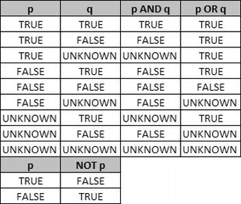
Figure 3-1. SQL 3VL Quick Reference Chart
As mentioned previously, the unknown logic values shown in the chart are the result of comparisons with NULL. The following predicates, for example, all evaluate to an unknown result:
@x  =  NULL
FirstName <> NULL
PhoneNumber  >  NULL
If you used one of these as the predicate in a WHERE clause of a SELECT statement, the statement would return no rows at all—SELECT with a WHERE clause returns only rows where the WHERE clause predicate evaluates to true; it discards rows for which the WHERE clause is false or unknown. Similarly, the INSERT, UPDATE, and DELETE statements with a WHERE clause only affect rows for which the WHERE clause evaluates to true.
SQL Server provides a proprietary mechanism, the SET ANSI_NULLS OFF option, to allow direct equality comparisons with NULL using the = and <> operators. The only ISO-compliant way to test for NULL is with the IS NULL and IS NOT NULL comparison predicates. We highly recommend that you stick with the ISO-compliant IS NULL and IS NOT NULL predicates for a few reasons:
- Many SQL Server features like computed columns, indexed views, and XML indexes require SET ANSI_NULLS ON at creation time.
- Mixing and matching SET ANSI_NULLS settings within your database can confuse other developers who have to maintain your code. Using ISO-compliant NULL-handling consistently eliminates confusion.
- SET ANSI_NULLS OFF allows direct equality comparisons with NULL, returning true if you compare a column or variable to NULL. It does not return true if you compare NULLs contained in two columns, though, which can be confusing.
- To top it all off, Microsoft has deprecated the SET ANSI_NULLS OFF setting. It will be removed in a future version of SQL Server, so it’s a good idea to start future-proofing your code now.
IT’S A CLOSED WORLD, AFTER ALL
The closed-world assumption (CWA) is an assumption in logic that the world is “black and white,” “true and false,” or “ones and zeros.” When applied to databases, the CWA basically states that all data stored within the database is true; everything else is false. The CWA presumes that only knowledge of the world that is complete can be stored within a database.
NULL introduces an open-world assumption (OWA) into the mix. It allows you to store information in the database that may or may not be true. This means that an SQL database can store incomplete knowledge of the world—a direct violation of the CWA. Many relational management (RM) theorists see this as an inconsistency in the SQL DBMS model. This argument fills many an RM textbook and academic blog, including web sites like Hugh Darwen and C. J. Date’s “The Third Manifesto” (www.thethirdmanifesto.com/), so we won’t go deeply into the details here. Just realize that many RM experts dislike SQL NULL. As an SQL practitioner in the real world, however, you may discover that NULL is often the best option available to accomplish many tasks.
T-SQL implements procedural language control-of-flow statements, including such constructs as BEGIN. . .END, IF. . .ELSE, WHILE, and GOTO. T-SQL’s control-of-flow statements provide a framework for developing rich server-side procedural code. Procedural code in T-SQL does come with some caveats, though, which we will discuss in this section.
T-SQL uses the keywords BEGIN and END to group multiple statements together in a statement block. The BEGIN and END keywords don’t alter execution order of the statements they contain, nor do they define an atomic transaction, limit scope, or perform any function other than defining a simple grouping of T-SQL statements.
Unlike other languages, such as C++ or C#, which use braces ({ }) to group statements in logical blocks, T-SQL’s BEGIN and END keywords do not define or limit scope. The following sample C# code, for instance, will not even compile:
{
int j  =  10; } Console.WriteLine (j);
C# programmers will automatically recognize that the variable j in the previous code is defined inside braces, limiting its scope and making it accessible only inside the braces. T-SQL’s roughly equivalent code, however, does not limit scope in this manner:
BEGIN
    DECLARE @j int  =  10;
END
PRINT @j;
The previous T-SQL code executes with no problem, as long as the DECLARE statement is encountered before the variable is referenced in the PRINT statement. The scope of variables in T-SQL is defined in terms of command batches and database object definitions (such as SPs, UDFs, and triggers). Declaring two or more variables with the same name in one batch or SP will result in errors.
![]() Caution T-SQL’s BEGIN and END keywords create a statement block but do not define a scope. Variables declared inside a BEGIN. . .END block are not limited in scope just to that block, but are scoped to the whole batch, SP, or UDF in which they are defined.
Caution T-SQL’s BEGIN and END keywords create a statement block but do not define a scope. Variables declared inside a BEGIN. . .END block are not limited in scope just to that block, but are scoped to the whole batch, SP, or UDF in which they are defined.
BEGIN. . .END is useful for creating statement blocks where you want to execute multiple statements based on the results of other control-of-flow statements like IF. . .ELSE and WHILE. BEGIN. . .END can also have another added benefit if you’re using SSMS 2012 or a good third-party SQL editor like ApexSQL Edit (www.apexsql.com/). In advanced editors like these, BEGIN. . .END can alert the GUI that a section of code is collapsible, as shown in Figure 3-2. This can speed up development and ease debugging, especially if you’re writing complex T-SQL scripts.

Figure 3-2. BEGIN. . .END Statement Blocks Marked Collapsible in ApexSQL Edit
![]() Tip Although it’s not required, we like to wrap the body of CREATE PROCEDURE statements with BEGIN. . .END. This clearly delineates the bodies of the SPs, separating them from other code in the same script.
Tip Although it’s not required, we like to wrap the body of CREATE PROCEDURE statements with BEGIN. . .END. This clearly delineates the bodies of the SPs, separating them from other code in the same script.
Like many procedural languages, T-SQL implements conditional execution of code using the simplest of procedural statements: the IF. . .ELSE construct. The IF statement is followed by a logical predicate. If the predicate evaluates to true, the single SQL statement or statement blocked wrapped in BEGIN. . .END is executed. If the predicate evaluates to either false or unknown, SQL Server falls through to the ELSE statement and executes the single statement or statement block following ELSE.
![]() Tip A predicate in SQL is an expression that evaluates to one of the logical results true, false, or unknown. Predicates are used in IF. . .ELSE statements, WHERE clauses, and anywhere that a logical result is needed.
Tip A predicate in SQL is an expression that evaluates to one of the logical results true, false, or unknown. Predicates are used in IF. . .ELSE statements, WHERE clauses, and anywhere that a logical result is needed.
The example in Listing 3-1 performs up to three comparisons to determine whether a variable is equal to a specified value. The second ELSE statement executes if and only if the tests for both true and false conditions fail.
Listing 3-1. Simple IF . . . ELSE Example
DECLARE @i int  =  NULL;
IF @i  =  10
    PRINT 'TRUE.';
ELSE IF NOT (@i  =  10)
    PRINT 'FALSE.';
ELSE
    PRINT 'UNKNOWN.';
Because the variable @i is NULL in the example, SQL Server reports that the result is unknown. If you assign the value 10 to the variable @i, SQL Server will report that the result is true; all other values will report false.
To create a statement block containing multiple T-SQL statements after either the IF statement or the ELSE statement, simply wrap your statements with the T-SQL BEGIN and END keywords discussed in the previous section. The simple example in Listing 3-2 is an IF. . .ELSE statement with statement blocks. The example uses IF. . .ELSE to check the value of the variable @direction. If @direction is ASCENDING, a message is printed, and the top ten names, in order of last name, are selected from the Person.Contact table. If @direction is DESCENDING, a different message is printed, and the bottom ten names are selected from the Person.Contact table. Any other value results in a message that @direction was not recognized. The results of Listing 3-2 are shown in Figure 3-3.
Listing 3-2. IF . . . ELSE with Statement Blocks
DECLARE @direction NVARCHAR(20)  =  N'DESCENDING';

IF @direction  =  N'ASCENDING'
BEGIN
        PRINT 'Start at the top!';

        SELECT TOP (10)
        LastName,
        FirstName,
        MiddleName
        FROM Person.Person
        ORDER BY LastName ASC;
END
ELSE  IF @direction  =  N'DESCENDING'
BEGIN
        PRINT 'Start at the bottom!';

        SELECT TOP (10)
        LastName,
        FirstName,
        MiddleName
        FROM Person.Person
        ORDER BY LastName DESC;
END
ELSE
PRINT '@direction was not recognized!';

Figure 3-3. The Last Ten Contact Names in the AdventureWorks Database
The WHILE, BREAK, and CONTINUE Statements
Looping is a standard feature of procedural languages, and T-SQL provides looping support through the WHILE statement and its associated BREAK and CONTINUE statements. The WHILE loop is immediately followed by a predicate, and WHILE will execute a given SQL statement or statement block bounded by the BEGIN and END keywords as long as the associated predicate evaluates to true. If the predicate evaluates to false or unknown, the code in the WHILE loop will not execute and control will pass to the next statement after the WHILE loop. The WHILE loop in Listing 3-3 is a very simple example that counts from 1 to 10. The result is shown in Figure 3-4.
Listing 3-3. WHILE Statement Example
DECLARE @i int  =  1;
WHILE @i <  = 10
BEGIN
   PRINT @i;
   SET @i  =  @i  +  1;
END

Figure 3-4. Counting from 1 to 10 with WHILE
![]() Tip Be sure to update your counter or other flag inside the WHILE loop. The WHILE statement will keep looping until its predicate evaluates to false or unknown. A simple coding mistake could create a nasty infinite loop.
Tip Be sure to update your counter or other flag inside the WHILE loop. The WHILE statement will keep looping until its predicate evaluates to false or unknown. A simple coding mistake could create a nasty infinite loop.
T-SQL also includes two additional keywords that can be used with the WHILE statement: BREAK and CONTINUE. The CONTINUE keyword forces the WHILE loop to immediately jump to the start of the code block, as in the modified example in Listing 3-4.
Listing 3-4. WHILE . . . CONTINUE Example
DECLARE @i int  =  1;
WHILE @i <  = 10
BEGIN
   PRINT @i;
   SET @i  =  @i  +  1;

CONTINUE; -- Force the WHILE loop to restart

PRINT 'The CONTINUE keyword ensures that this will never be printed.';

END
The BREAK keyword, on the other hand, forces the WHILE loop to terminate immediately. In Listing 3-5, BREAK forces the WHILE loop to exit during the first iteration so that the numbers 2 through 10 are never printed.
Listing 3-5. WHILE . . . BREAK Example
DECLARE @i int  =  1;
WHILE @i <  = 10
BEGIN
   PRINT @i;
   SET @i  =  @i  +  1;

   BREAK; -- Force the WHILE loop to terminate

   PRINT 'The BREAK keyword ensures that this will never be printed.';
END
![]() Tip BREAK and CONTINUE can and should be avoided in most cases. It’s not uncommon to see a WHILE l = l statement with a BREAK in the body of the loop. This can always be rewritten, usually very easily, to remove the BREAK statement. Most of the time, the BREAK and CONTINUE keywords introduce additional complexity to your logic and cause more problems than they solve.
Tip BREAK and CONTINUE can and should be avoided in most cases. It’s not uncommon to see a WHILE l = l statement with a BREAK in the body of the loop. This can always be rewritten, usually very easily, to remove the BREAK statement. Most of the time, the BREAK and CONTINUE keywords introduce additional complexity to your logic and cause more problems than they solve.
Despite Edsger W. Dijkstra’s best efforts at warning developers (see Dijkstra’s 1968 letter, “Go To Statement Considered Harmful”), T-SQL still has a GOTO statement. The GOTO statement transfers control of your program to a specified label unconditionally. Labels are defined by placing the label identifier on a line followed by a colon (:), as shown in Listing 3-6. This simple example executes its step 1 and uses GOTO to dive straight into step 3, skipping step 2. The results are shown in Figure 3-5.
Listing 3-6. Simple GOTO Example
PRINT 'Step 1 Begin.';
GOTO Step3_Label;

PRINT 'Step 2 will not be printed.';

Step3_Label:
PRINT 'Step 3 End.';

Figure 3-5. GOTO Statement Transfers Control Unconditionally
The GOTO statement is best avoided, since it can quickly degenerate your programs into unstructured spaghetti code. When you have to write procedural code, you’re much better off using structured programming constructs like IF. . .ELSE and WHILE statements.
The WAITFOR Statement
The WAITFOR statement suspends execution of a transaction, SP, or T-SQL command batch until a specified time is reached, a time interval has elapsed, or a message is received from Service Broker.
![]() Note Service Broker is an SQL Server messaging system. We don’t detail Service Broker in this book, but you can find out more about it in Pro SQL Server 2008 Service Broker, by Klaus Aschenbrenner and Remus Rusana (Apress, 2008).
Note Service Broker is an SQL Server messaging system. We don’t detail Service Broker in this book, but you can find out more about it in Pro SQL Server 2008 Service Broker, by Klaus Aschenbrenner and Remus Rusana (Apress, 2008).
The WAITFOR statement has a DELAY option that tells SQL Server to suspend code execution until one of the following criteria is met or a specified time interval has elapsed. The time interval is specified as a valid time string in the format hh:mm:ss. The time interval cannot contain a date portion; it must only include the time, and it can be up to 24 hours. Listing 3-7 is an example of the WAITFOR statement with the DELAY option, which blocks execution of the batch for 3 seconds.
WAITFOR CAVEATS
There are some caveats associated with the WAITFOR statement. In some situations, WAITFOR can cause longer delays than the interval you specify. SQL Server also assigns each WAITFOR statement its own thread, and if SQL Server begins experiencing thread starvation, it can randomly stop WAITFOR threads to free up thread resources. If you need to delay execution for an exact amount of time, you can guarantee more consistent results by suspending execution through an external application like SSIS.
In addition to its DELAY and TIME options, you can use WAITFOR with the RECEIVE and GET CONVERSATION GROUP options with Service Broker-enabled applications. When you use WAITFOR with RECEIVE, the statement waits for receipt of one or more messages from a specified queue.
When you use WAITFOR with the GET CONVERSATION GROUP option, it waits for a conversation group identifier of a message. GET CONVERSATION GROUP allows you to retrieve information about a message and lock the conversation group for the conversation containing the message, all before retrieving the message itself.
A detailed description of Service Broker is beyond the scope of this book, but Accelerated SQL Server 2008, by Rob Walters et al. (Apress, 2008) gives a good description of Service Broker functionality and options still applicable to SQL Server 2012.
Listing 3-7. WAITFOR Example
PRINT 'Step 1 complete. ';
GO

DECLARE @time_to_pass nvarchar(8);
SELECT @time_to_pass  =  N'00:00:03';
WAITFOR DELAY @time_to_pass;
PRINT 'Step 2 completed three seconds later. ';
You can also use the TIME option with the WAITFOR statement. If you use the TIME option, SQL Server will wait until the appointed time before allowing execution to continue. Datetime variables are allowed, but the date portion is ignored when the TIME option is used.
The RETURN statement exits unconditionally from an SP or command batch. When you use RETURN, you can optionally specify an integer expression as a return value. The RETURN statement returns a given integer expression to the calling routine or batch. If you don’t specify an integer expression to return, a value of 0 is returned by default. RETURN is not normally used to return calculated results, except for UDFs, which offer more RETURN options (we will detail these in Chapter 4). For SPs and command batches, the RETURN statement is used almost exclusively to return a success indicator, failure indicator, or error code.
WHAT NUMBER, SUCCESS?
All system SPs return 0 to indicate success, or a nonzero value to indicate failure (unless otherwise documented in BOL). It is considered bad form to use the RETURN statement to return anything other than an integer status code from a script or SP.
UDFs, on the other hand, have their own rules. UDFs have a flexible variation of the RETURN statement, which exits the body of the UDF. In fact, a UDF requires the RETURN statement be used to return scalar or tabular results to the caller. You will see UDFs again in detail in Chapter 4.
![]() Note There are a couple of methods in T-SQL to redirect logic flow based on errors. These include the TRY. . .CATCH statement and the THROW statement. Both statements will be discussed in detail in Chapter 17.
Note There are a couple of methods in T-SQL to redirect logic flow based on errors. These include the TRY. . .CATCH statement and the THROW statement. Both statements will be discussed in detail in Chapter 17.
The CASE Expression
The T-SQL CASE function is SQL Server’s implementation of the ISO SQL CASE expression. While the previously discussed T-SQL control-of-flow statements allow for conditional execution of SQL statements or statement blocks, the CASE expression allows for set-based conditional processing inside a single query. CASE provides two syntaxes, simple and searched, which we will discuss in this section.
The Simple CASE Expression
The simple CASE expression returns a result expression based on the value of a given input expression. The simple CASE expression compares the input expression to a series of expressions following WHEN keywords. Once a match is encountered, CASE returns a corresponding result expression following the keyword THEN. If no match is found, the expression following the keyword ELSE is returned, and NULL is returned if no ELSE keyword is supplied.
Consider the example in Listing 3-8, which uses a simple CASE expression to count all the AdventureWorks customers on the West Coast (which we arbitrarily defined as the states of California, Washington, and Oregon). The query also uses a CTE (common table expression) which we will discuss more thoroughly in Chapter 8. The results are shown in Figure 3-6.
Listing 3-8. Counting West Coast Customers with a Simple CASE Expression
WITH  EmployeesByRegion(Region)
AS
(
    SELECT
        CASE sp.StateProvinceCode
        WHEN 'CA' THEN 'West Coast'
        WHEN 'WA' THEN 'West Coast'
        WHEN 'OR' THEN 'West Coast'
        ELSE 'Elsewhere'
        END
    FROM  HumanResources.Employee e
    INNER JOIN Person.Person p
        ON e.BusinessEntityID  =  p.BusinessEntityID
       INNER JOIN Person.BusinessEntityAddress bea
              ON bea.BusinessEntityID  =  e.BusinessEntityID
       INNER JOIN Person.Address a
           ON a.AddressID  =  bea.AddressID
       INNER JOIN Person.StateProvince sp
              ON sp.StateProvinceID  =  a.StateProvinceID
    WHERE sp.CountryRegionCode  =  'US'
)
SELECT  COUNT(Region)  AS  NumOfEmployees,  Region
FROM    EmployeesByRegion
GROUP BY Region;
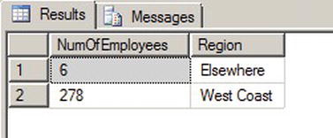
Figure 3-6. Results of the West Coast Customer Count
The CASE expression in the subquery compares the StateProvinceCode value to each of the state codes following the WHEN keywords, returning the name West Coast when the StateProvinceCode is equal to CA, WA, or OR. For any other StateProvinceCode in the United States, it returns a value of Elsewhere.
SELECT CASE sp.StateProvinceCode
        WHEN 'CA' THEN 'West Coast'
        WHEN 'WA' THEN 'West Coast'
        WHEN 'OR' THEN 'West Coast'
        ELSE 'Elsewhere'
    END
The remainder of the example simply counts the number of rows returned by the query, grouped by Region.
A SIMPLE CASE OF NULL
The simple CASE expression performs basic equality comparisons between the input expression and the expressions following the WHEN keywords. This means that you cannot use the simple CASE expression to check for NULLs. Recall from the “Three-Valued Logic” section of this chapter that a NULL, when compared to anything, returns unknown. The simple CASE expression only returns the expression following the THEN keyword when the comparison returns true. This means that if you ever try to use NULL in a WHEN expression, the corresponding THEN expression will not be returned. If you need to check for NULL in a CASE expression, use a searched CASE expression with the IS NULL or IS NOT NULL comparison operators.
The searched CASE expression provides a mechanism for performing more complex comparisons. The searched CASE evaluates a series of predicates following WHEN keywords until it encounters one that evaluates to true. At that point, it returns the corresponding result expression following the THEN keyword. If none of the predicates evaluates to true, the result following the ELSE keyword is returned. If none of the predicates evaluates to true and ELSE is not supplied, the searched CASE expression returns NULL.
Predicates in the searched CASE expression can take advantage of any valid SQL comparison operators (e.g., <, >, =, LIKE, and IN). The simple CASE expression from Listing 3-8 can be easily expanded to cover multiple geographic regions using the searched CASE expression and the IN logical operator, as shown in Listing 3-9. This example uses a searched CASE expression to group states into West Coast, Pacific, and New England regions. The results are shown in Figure 3-7.
Listing 3-9. Counting Employees by Region with a Searched CASE Expression
WITH  EmployeesByRegion(Region)
AS
(
    SELECT
        CASE WHEN sp.StateProvinceCode IN ('CA', 'WA', 'OR') THEN 'West Coast'
        WHEN sp.StateProvinceCode IN ('HI', 'AK') THEN 'Pacific'
        WHEN  sp.StateProvinceCode  IN  ('CT',  'MA', 'ME', 'NH', 'RI', 'VT')
        THEN 'New England'
        ELSE 'Elsewhere'
        END
    FROM  HumanResources.Employee e
    INNER JOIN Person.Person p
        ON e.BusinessEntityID  =  p.BusinessEntityID
       INNER JOIN Person.BusinessEntityAddress bea
           ON bea.BusinessEntityID  =  e.BusinessEntityID
       INNER JOIN Person.Address a
           ON a.AddressID  =  bea.AddressID
       INNER JOIN Person.StateProvince sp
           ON sp.StateProvinceID  =  a.StateProvinceID
    WHERE sp.CountryRegionCode  =  'US'
)
SELECT  COUNT(Region)  AS  NumOfCustomers,  Region
FROM    EmployeesByRegion
GROUP BY Region;
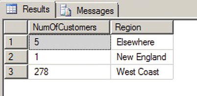
Figure 3-7. Results of the Regional Customer Count
The searched CASE expression in the example uses the IN operator to return the geographic area that StateProvinceCode is in: California, Washington, and Oregon all return West Coast; and Connecticut, Massachusetts, Maine, New Hampshire, Rhode Island, and Vermont all return New England. If the StateProvinceCode does not fit in one of these regions, the searched CASE expression will return Elsewhere.
SELECT
    CASE WHEN sp.StateProvinceCode IN ('CA', 'WA', 'OR') THEN 'West Coast'
        WHEN sp.StateProvinceCode IN ('HI', 'AK') THEN 'Pacific'
        WHEN  sp.StateProvinceCode  IN  ('CT',  'MA', 'ME', 'NH', 'RI', 'VT')
        THEN 'New England'
        ELSE  'Elsewhere'
    END
The balance of the sample code in Listing 3-9 counts the rows returned, grouped by Region. The CASE expression, either simple or searched, can be used in SELECT, UPDATE, INSERT, MERGE, and DELETE statements.
A CASE BY ANY OTHER NAME
Many programming and query languages offer expressions that are analogous to the SQL CASE expression. C++ and C#, for instance, offer the ?: operator, which fulfills the same function as a searched CASE expression. XQuery has its own flavor of if. . .then. . .else expression that is also equivalent to the SQL searched CASE.
C# and Visual Basic also supply the switch and Select statements, respectively, which are semi-analogous to SQL’s simple CASE expression. The main difference, of course, is that SQL’s CASE expression simply returns a scalar value, while the C# and Visual Basic statements actually control program flow, allowing you to execute statements based on an expression’s value. The similarities and differences between SQL expressions and statements and similar constructs in other languages provide a great starting point for learning the nitty-gritty details of T-SQL.
Many times, business reporting requirements dictate that a result should be returned in pivot table format. Pivot table format simply means that the labels for columns and/or rows are generated from the data contained in rows. Microsoft Access and Excel users have long had the ability to generate pivot tables on their data, and SQL Server 2012 supports the PIVOT and UNPIVOT operators introduced in SQL Server 2005. Back in the days of SQL Server 2000 and before, however, CASE expressions were the only method of generating pivot table-type queries. And even though SQL Server 2012 provides the PIVOT and UNPIVOT operators, truly dynamic pivot tables still require using CASE expressions and dynamic SQL. The static pivot table query shown in Listing 3-10 returns a pivot table-formatted result with the total number of orders for each AdventureWorks sales region in the United States. The results are shown in Figure 3-8.
Listing 3-10. CASE-Style Pivot Table
SELECT
    t.CountryRegionCode,
    SUM
    (
        CASE WHEN t.Name  =  'Northwest' THEN 1
        ELSE    0
        END
    )  AS       Northwest,
    SUM
    (
        CASE WHEN t.Name  =  'Northeast' THEN 1
        ELSE    0
        END
    )  AS       Northeast,
    SUM
    (
        CASE WHEN t.Name  =  'Southwest' THEN 1
        ELSE    0
        END
    )  AS       Southwest,
    SUM
    (
        CASE WHEN t.Name  =  'Southeast' THEN 1
        ELSE    0
        END
    )  AS       Southeast,
    SUM
    (
        CASE WHEN t.Name  =  'Central' THEN 1
        ELSE    0
        END
    )  AS  Central
FROM  Sales.SalesOrderHeader soh
INNER  JOIN  Sales.SalesTerritory  t
    ON  soh.TerritoryID  =  t.TerritoryID
WHERE  t.CountryRegionCode  =  'US'
GROUP  BY  t.CountryRegionCode;

Figure 3-8. Number of Sales by Region in Pivot Table Format
This type of static pivot table can also be used with the SQL Server 2012 PIVOT operator. The sample code in Listing 3-11 uses the PIVOT operator to generate the same result as the CASE expressions in Listing 3-10.
Listing 3-11. PIVOT Operator Pivot Table
SELECT
    CountryRegionCode,
    Northwest,
    Northeast,
    Southwest,
    Southeast,
    Central
FROM
(
    SELECT
        t.CountryRegionCode,
        t.Name
    FROM  Sales.SalesOrderHeader  soh
    INNER JOIN Sales.SalesTerritory t
        ON  soh.TerritoryID  =  t.TerritoryID
    WHERE t.CountryRegionCode  =  'US'
)  p
PIVOT
(
    COUNT (Name)
    FOR  Name
    IN
    (
        Northwest,
        Northeast,
        Southwest,
        Southeast,
        Central
    )
)  AS  pvt;
On occasion, you might need to run a pivot table-style report where you don’t know the column names in advance. This is a dynamic pivot table script that uses a temporary table and dynamic SQL to generate a pivot table, without specifying the column names in advance. Listing 3-12 demonstrates one method of generating dynamic pivot tables in T-SQL. The results are shown in Figure 3-9.
Listing 3-12. Dynamic Pivot Table Query
-- Declare variables
DECLARE @sql nvarchar(4000);

DECLARE @temp_pivot table
 (
  TerritoryID int NOT NULL PRIMARY KEY,
  CountryRegion nvarchar(20) NOT NULL,
  CountryRegionCode nvarchar(3) NOT NULL
 );

-- Get column names from source table rows
INSERT INTO @temp_pivot
 (
  TerritoryID,
  CountryRegion,
  CountryRegionCode
 )
 SELECT
  TerritoryID,
  Name,
  CountryRegionCode
  FROM Sales.SalesTerritory
  GROUP BY
     TerritoryID,
     Name,
     CountryRegionCode;

-- Generate dynamic SQL query
SET @sql  =  N'SELECT' +
    SUBSTRING(
       (
         SELECT N', SUM(CASE WHEN t.TerritoryID  =  ' +
           CAST(TerritoryID AS NVARCHAR(3)) +
        N' THEN 1 ELSE 0 END) AS '  +  QUOTENAME(CountryRegion) AS "*"
        FROM @temp_pivot
        FOR XML PATH('')
    ), 2, 4000) +
    N' FROM Sales.SalesOrderHeader soh ' +
       N' INNER JOIN Sales.SalesTerritory t ' +
       N' ON soh.TerritoryID  =  t.TerritoryID; ' ;

-- Print and execute dynamic SQL
PRINT @sql;
EXEC (@sql);
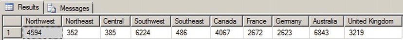
Figure 3-9. Dynamic Pivot Table Result
The script in Listing 3-12 first declares an nvarchar variable that will hold the dynamically generated SQL script and a table variable that will hold all of the column names, which are retrieved from the row values in the source table.
-- Declare variables
DECLARE @sql nvarchar(4000);

DECLARE @temp_pivot table
 (
  TerritoryID int NOT NULL PRIMARY KEY,
  CountryRegion nvarchar(20) NOT NULL,
  CountryRegionCode nvarchar(3) NOT NULL
 );
Next, the script grabs a list of distinct territory-specific values from the table and stores them in the @temp_pivot table variable. These values from the table will become column names in the pivot table result.
-- Get column names from source table rows
INSERT INTO @temp_pivot
 (
  TerritoryID,
  CountryRegion,
  CountryRegionCode
 )
 SELECT
  TerritoryID,
  Name,
  CountryRegionCode
  FROM Sales.SalesTerritory
  GROUP BY
     TerritoryID,
     Name,
     CountryRegionCode;
The script then uses FOR XML PATH to efficiently generate the dynamic SQL SELECT query that contains CASE expressions and column names generated dynamically based on the values in the @temppivot table variable. This SELECT query will create the dynamic pivot table result.
-- Generate dynamic SQL query
SET @sql  =  N'SELECT' +
    SUBSTRING(
       (
         SELECT N', SUM(CASE WHEN t.TerritoryID  =  ' +
           CAST(TerritoryID AS NVARCHAR(3)) +
        N' THEN 1 ELSE 0 END) AS '  +  QUOTENAME(CountryRegion) AS "*"
        FROM @temp_pivot
        FOR XML PATH('')
    ), 2, 4000) +
    N' FROM Sales.SalesOrderHeader soh ' +
       N' INNER JOIN Sales.SalesTerritory t ' +
       N' ON soh.TerritoryID  =  t.TerritoryID; ' ;
Finally, the dynamic pivot table query is printed out and executed with the T-SQL PRINT and EXEC statements.
-- Print and execute dynamic SQL
PRINT @sql;
EXEC (@sql);
Listing 3-13 shows the dynamic SQL pivot table query generated by the code in Listing 3-12.
Listing 3-13. Autogenerated Dynamic SQL Pivot Table Query
SELECT SUM
(
    CASE  WHEN  t.TerritoryID  =  1  THEN       1
        ELSE 0
    END
)  AS   [Northwest],
SUM
(
    CASE  WHEN  t.TerritoryID  =  2  THEN       1
        ELSE 0
    END
)  AS   [Northeast],
SUM
(
    CASE  WHEN  t.TerritoryID  =  3  THEN       1
        ELSE 0
    END
)  AS  [Central],
SUM
(
    CASE  WHEN  t.TerritoryID  =  4  THEN       1
        ELSE 0
    END
)  AS   [Southwest],
SUM
(
    CASE  WHEN  t.TerritoryID  =  5  THEN       1
        ELSE 0
    END
)  AS   [Southeast],
SUM
(
    CASE  WHEN  t.TerritoryID  =  6  THEN       1
        ELSE 0
    END
)  AS  [Canada],
SUM
(
    CASE  WHEN  t.TerritoryID  =  7  THEN       1
        ELSE 0
    END
)  AS  [France],
SUM
(
    CASE  WHEN  t.TerritoryID  =  8  THEN       1
        ELSE 0
    END
)  AS  [Germany],
SUM
(
    CASE  WHEN  t.TerritoryID  =  9  THEN       1
        ELSE 0
    END
)  AS  [Australia],
SUM
(
    CASE  WHEN  t.TerritoryID  =  10  THEN       1
        ELSE 0
    END
)  AS  [United Kingdom]
FROM  Sales.SalesOrderHeader soh
INNER  JOIN  Sales.SalesTerritory  t
    ON  soh.TerritoryID  =  t.TerritoryID;
![]() Caution Anytime you use dynamic SQL, make sure that you take precautions against SQL injection—that is, malicious SQL code being inserted into your SQL statements. In this instance, we’re using the QUOTENAME function to quote the column names being dynamically generated to help avoid SQL injection problems. We’ll cover dynamic SQL and SQL injection in greater detail in Chapter 17.
Caution Anytime you use dynamic SQL, make sure that you take precautions against SQL injection—that is, malicious SQL code being inserted into your SQL statements. In this instance, we’re using the QUOTENAME function to quote the column names being dynamically generated to help avoid SQL injection problems. We’ll cover dynamic SQL and SQL injection in greater detail in Chapter 17.
SQL Server 2012 simplifies the standard CASE statement by introducing the concept of an IIF statement. You get the same results as you would using the CASE statement but with much less code. Those familiar with Microsoft .NET will be glad to see the same functionality is now part of T-SQL.
The syntax is simple. The command takes a Boolean expression, a value when the expression equates to true and a value when the expression equates to false. Listing 3-14 show two examples. One example uses variables and the other uses table columns. The output for both statements is shown in Figure 3-10.
Listing 3-14. Examples Using the IIF statement
--Example 1. IIF Statement Using Variables

DECLARE @valueA int  =  85
DECLARE @valueB int  =  45

SELECT IIF (@valueA  <  @valueB, 'True', 'False') AS Result

--Example 2. IIF Statement Using Table Column

SELECT IIF (Name in ('Alberta', 'British Columbia'), 'Canada', Name)
FROM [Person].[StateProvince]

Figure 3-10. Partial Output of IIF Statements
CHOOSE
Another logical function introduced in SQL Server 2012 is the CHOOSE function. The CHOOSE function allows you to select a member of an array based on an integer index value. Simply put, the CHOOSE function lets you select a member from a list. The member you select can either be based off a static index value or computed value. The syntax for the CHOOSE function is as follows:
CHOOSE ( index, val_1, val_2 [, val_n ] )
If the index value is not an integer (let’s say it’s a decimal), then SQL will convert it to an integer. If the index value is out of range for the index, then the function will return a NULL. Listing 3-15 shows a simple example and Figure 3-11 shows the output. The example uses the integer value of the PhoneNumberTypeID to determine the type of phone. In this case the phone type is defined in the table so a CHOOSE function would not be necessary but in other cases the value may not be defined.
Listing 3-15. Example Using the CHOOSE Statement
SELECT p.FirstName,
       pp.PhoneNumber,
       CHOOSE(pp.PhoneNumberTypeID, 'Cell', 'Home', 'Work') 'Phone Type'
FROM Person.Person p
JOIN Person.PersonPhone pp
ON p.BusinessEntityID  =  pp.BusinessEntityID
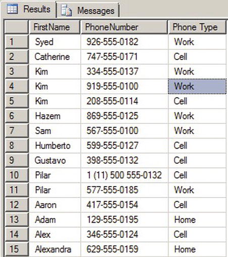
Figure 3-11. Partial Output of CHOOSE Statement
The COALESCE function takes a list of expressions as arguments and returns the first non-NULL value from the list. The COALESCE function is defined by ISO as shorthand for the following equivalent searched CASE expression:
CASE
WHEN expressionl IS NOT NULL THEN expression! WHEN expression IS NOT NULL THEN expression
[ .  .  . " ] END
The following COALESCE function example returns the value of MiddleName when MiddleName is not NULL, and the string No Middle Name when MiddleName is NULL:
COALESCE (MiddleName, 'No Middle Name')
The NULLIF function accepts exactly two arguments. NULLIF returns NULL if the two expressions are equal, and it returns the value of the first expression if the two expressions are not equal. NULLIF is defined by the ISO standard as equivalent to the following searched CASE expression:
CASE WHEN expressionl  =  expression2 THEN NULL
ELSE expressionl
END
NULLIF is often used in conjunction with COALESCE. Consider Listing 3-16, which combines COALESCE with NULLIF to return the string This is NULL or A if the variable @s is set to the character value A or NULL.
Listing 3-16. Using COALESCE with NULLIF
DECLARE @s varchar(10);
SELECT @s  =  'A';
SELECT COALESCE(NULLIF(@s, 'A'), 'This is NULL or A'),
T-SQL has long had alternate functionality similar to COALESCE. Specifically, the ISNULL function accepts two parameters and returns NULL if they are equal.
COALESCE OR ISNULL?
The T-SQL functions COALESCE and ISNULL perform similar functions, but which one should you use? COALESCE is more flexible than ISNULL and is compliant with the ISO standard to boot. This means that it is also the more portable option among ISO-compliant systems. COALESCE also implicitly converts the result to the data type with the highest precedence from the list of expressions. ISNULL implicitly converts the result to the data type of the first expression. Finally, COALESCE is a bit less confusing than ISNULL, especially considering that there’s already a comparison operator called IS NULL. In general, we recommend using the COALESCE function instead of ISNULL.
The word cursor comes from the Latin word for runner, and that is exactly what a T-SQL cursor does: it “runs” through a result set, returning one row at a time. Many T-SQL programming experts rail against the use of cursors for a variety of reasons—the chief among these include the following:
- Cursors use a lot of overhead, often much more than an equivalent set-based approach.
- Cursors override SQL Server’s built-in query optimizations, often making them much slower than an equivalent set-based solution.
Because cursors are procedural in nature, they are often the slowest way to manipulate data in T-SQL. Rather than spend the balance of the chapter ranting against cursor use, however, we’d like to introduce T-SQL cursor functionality and play devil’s advocate to point out some areas where cursors provide an adequate solution.
The first such area where we can recommend the use of cursors is in scripts or procedures that perform administrative tasks. In administrative tasks, the following items often hold true:
- Unlike normal data queries and data manipulations that are performed dozens, hundreds, or potentially thousands of times per day, administrative tasks are often performed on a one-off basis or on a regular schedule like once per day.
- Administrative tasks often require calling an SP or executing a procedural code block once for each row when performing administrative tasks based on a table of entries.
- Administrative tasks generally don’t need to query or manipulate massive amounts of data to perform their jobs.
- The order of the steps in which administrative tasks are performed and the order of the database objects they touch are often important.
The sample SP in Listing 3-17 is an example of an administrative task performed with a T-SQL cursor. The sample uses a cursor to loop through all indexes on all user tables in the current database. It then creates dynamic SQL statements to rebuild every index whose fragmentation level is above a user-specified threshold. The results are shown in Figure 3-12. Be aware that your results may return different values for each row.
Listing 3-17. Sample Administrative Task Performed with a Cursor
CREATE PROCEDURE dbo.RebuildIndexes
@ShowOrRebuiId nvarchar(10)  =  N'show',
@MaxFrag decimal(20, 2)  =  20.0
AS
BEGIN
-- Declare variables
SET NOCOUNT ON;

DECLARE
   @Schema nvarchar(128),
   @Table nvarchar(128),
   @Index nvarchar(128),
   @Sql nvarchar(4000),
   @DatabaseId int,
   @SchemaId int,
   @TableId int,
   @lndexId int;

-- Create the index list table
DECLARE @IndexList TABLE
(
   DatabaseName nvarchar(128) NOT NULL,
   DatabaseId int NOT NULL,
   SchemaName nvarchar(128) NOT NULL,
   SchemaId int NOT NULL,
   TableName nvarchar(128) NOT NULL,
   TableId int NOT NULL,
   IndexName nvarchar(128),
   IndexId int NOT NULL,
   Fragmentation decimal(20, 2),
PRIMARY KEY (DatabaseId, SchemaId, TableId, IndexId) );

-- Populate index list table
INSERT INTO @IndexList
(
   DatabaseName,
   DatabaseId,
   SchemaName,
   SchemaId,
   TableName,
   TableId,
   IndexName,
   IndexId,
   Fragmentation
)
SELECT
   db_name(),
   db_id(),
   s.Name,
   s.schema_id,
   t.Name,
   t.object_id,
   i.Name,
   i.index_id,
MAX(ip.avg_fragmentation_in_percent) FROM sys.tables t INNER JOIN sys.schemas s
ON t.schema_id  =  s.schema_id INNER JOIN sys.indexes i
ON t.object_id  =  i.object_id INNER JOIN sys.dm_db_index_physical_stats (db_id(), NULL, NULL, NULL, NULL) ip
ON ip.object_id  =  t.object_id AND ip.index_id  =  i.index_id WHERE ip.database_id  =  db_id()
 GROUP BY
   s.Name,
   s.schema_id,
   t.Name,
   t.object_id,
   i.Name,
   i.index_id;
-- If user specified rebuiId, use a cursor to loop through all indexes
-- rebuiId them
IF @ShowOrRebuiId  =  N'rebuiId'
BEGIN

-- Declare a cursor to create the dynamic SQL statements
DECLARE Index_Cursor CURSOR FAST_FORWARD
FOR SELECT SchemaName, TableName, IndexName
FROM @IndexList
WHERE Fragmentation  >  @MaxFrag
ORDER BY Fragmentation DESC, TableName ASC, IndexName ASC;

-- Open the cursor for reading
OPEN Index_Cursor;
-- Loop through all the tables in the database
FETCH NEXT FROM Index_Cursor
INTO @Schema, @Table, @Index;

WHILE @@FETCH_STATUS  =  0 BEGIN -- Create ALTER INDEX statement to rebuiId inddex
SET @Sql  =  N'ALTER INDEX ' +
 QUOTENAME(RTRIM(@Index))  +  N' ON '  +  QUOTENAME(RTRIM(@Table))  +  N'.' +
 QUOTENAME(RTRIM(@Table))  +  N' REBUIId WITH (ONLINE  =  OFF); ';

PRINT @Sql;

-- Execute dynamic SQL
EXEC (@Sql);

-- Get the next index
FETCH NEXT FROM Index_Cursor
INTO @Schema, @Table, @Index;
END

-- Close and deallocate the cursor.
CLOSE Index_Cursor;
DEALLOCATE Index_Cursor;
END
-- Show results, including oId fragmentation and new fragmentation
-- after index rebuiId
SELECT
il.DatabaseName,
il.SchemaName,
il.TableName,
il.IndexName,
il.Fragmentation AS FragmentationStart,
MAX(
  CAST(ip.avg_fragmentation_in_percent AS DECIMAL(20, 2))
) AS FragmentationEnd
FROM @IndexList il
INNER JOIN sys.dm_db_index_physical_stats(@DatabaseId, NULL, NULL, NULL, NULL) ip
ON DatabaseId  =  ip.database_id
   AND TableId  =  ip.object_id
   AND IndexId  =  ip.index_id
GROUP BY
   il.DatabaseName,
   il.SchemaName,
   il.TableName,
   il.IndexName,
   il.Fragmentation ORDER BY
   Fragmentation DESC,
   TableName ASC,
   IndexName ASC;
  RETURN;
END
GO
-- Execute index rebuild stored procedure
EXEC dbo.RebuildIndexes N'rebuild', 30;
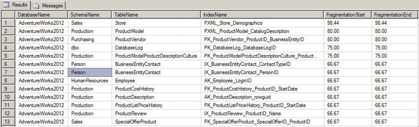
Figure 3-12. The Results of a Cursor-based Index Rebuild in the AdventureWorks Database
The dbo.RebuildIndexes procedure shown in Listing 3-17 populates a table variable with the information necessary to identify all indexes on all tables in the current database. It also uses the sys.dm_db_indexphysical_stats catalog function to retrieve initial index fragmentation information.
--Populate index list table

INSERT INTO @IndexList
(
DatabaseName,
DatabaseId,
SchemaName,
SchemaId,
TableName,
TableId,
IndexName,
IndexId,
Fragmentation
)
SELECT
  db_name(),
db_id(),
s.Name,
s.schema_id,
t.Name,
t.object_id,
i.Name,
i.index_id,
MAX(ip.avg_fragmentation_in_percent)
FROM sys.tables t
INNER JOIN sys.schemas s
  ON t.schema_id  =  s.schema_id
INNER JOIN sys.indexes i
  ON t.object_id  =  i.object_id
INNER JOIN sys.dm_db_index_physical_stats (db_id(), NULL, NULL,NULL, NULL) ip
ON ip.object_id  =  t.object_id
   AND ip.index_id  =  i.index_id
WHERE ip.database_id  =  db_id()
 GROUP BY
   s.Name,
   s.schema_id,
   t.Name,
   t.object_id,
   i.Name,
   i.index_id;
If you specify a rebuild action when you call the procedure, it creates a cursor to loop through the rows of the @IndexList table, but only for indexes with a fragmentation percentage higher than the level that you specified when calling the procedure.
-- Declare a cursor to create the dynamic SOL statements
DECLARE Index_Cursor CURSOR FAST_FORWARD
FOR
SELECT
  SchemaName,
  TableName,
  IndexName FROM @IndexList
WHERE Fragmentation  >  @MaxFrag
ORDER BY
  Fragmentation DESC,
  TableName ASC,
  IndexName ASC;
The procedure then loops through all the indexes in the @IndexList table, creating an ALTER INDEX statement to rebuild each index. Each ALTER INDEX statement is created as dynamic SQL to be printed and executed using the SQL PRINT and EXEC statements.
-- Open the cursor for reading
OPEN Index_Cursor;

-- Loop through all the tables in the database
FETCH NEXT FROM Index_Cursor
INTO @Schema,@Table, @Index;

WHILE @@FETCH_STATUS  =  0
BEGIN
 -- Create ALTER INDEX statement to rebuild index
SET @Sql  =  N'ALTER INDEX ' +
 QUOTENAME(RTRIM(@Index))  +  N' ON '  +  OUOTENAME(l@Schema)  +  N'.' +
 OUOTENAME(RTRIM(@Table))  +  N' REBUILD WITH (ONLINE  =  OFF); ';

PRINT @Sql;

-- Execute dynamic SQL
EXEC (@Sql);

-- Get the next index
FETCH NEXT FROM Index_Cursor
INTO @Schema, @Table, @lndex;
END

-- Close and deallocate the cursor.
CLOSE Index_Cursor;
DEALLOCATE Index_Cursor;
The dynamic SQL statements generated by the procedure look similar to the following:
ALTER INDEX [IX_PurchaseOrderHeader_EmployeeID]
ON [Purchasing].[PurchaseOrderHeader] REBUILD WITH (ONLINE  =  OFF);
The balance of the code simply displays the results, including the new fragmentation percentage after the indexes are rebuilt.
NO DBCC?
You’ll notice in the sample code in Listing 3-17 that we specifically avoided using database console commands (DBCCs) like DBCC DBREINDEX and DBCC SHOWCONTIG to manage index fragmentation and rebuild the indexes in the database. There’s a very good reason for this—these DBCC statements, and many others, are deprecated. Microsoft is planning to do away with many common DBCC statements in favor of catalog views and enhanced T-SQL statement syntax. The DBCC DBREINDEX statement, for instance, is now being replaced by the ALTER INDEX REBUILD syntax, and DBCC SHOWCONTIG is replaced by the sys.dm_db_index_physical_stats catalog function. Keep this in mind when porting code from legacy systems and creating new code.
Another situation where we would advise developers to use cursors is when the solution required is a one-off task, a set-based solution would be very complex, and time is short. Examples include creating complex running sum-type calculations or performing complex data-scrubbing routines on a very limited timeframe. We would not advise using a cursor as a permanent production application solution without exploring all available set-based options, however. Remember that whenever you use a cursor, you override SQL Server’s automatic optimizations; and the SQL Server query engine has much better and more current information to optimize operations than you will have access to at any given point in time. Also keep in mind that the tasks you consider extremely complex today will become much easier as SQL’s set-based processing becomes second nature to you.
CURSORS, CURSORS EVERYWHERE
Although cursors commonly get a lot of bad press from SQL gurus, there is nothing inherently evil about them. They are just another tool in the toolkit and should be viewed as such. What is wrong, however, is the ways in which developers abuse them. Generally speaking, and perhaps as much as 90 percent of the time, cursors are absolutely not the best tool for the job when you’re writing T-SQL code. Unfortunately, many SQL newbies find set-based logic difficult to grasp at first. Cursors provide a comfort zone for procedural developers because they lend themselves to procedural design patterns.
One of the worst design patterns you can adopt is the “cursors, cursors everywhere” design pattern. Believe it or not, there are people out there who have been writing SQL code for years and have never bothered learning about SQL’s set-based processing. These people tend to approach every SQL problem as if it were a C# or Visual Basic problem, and their code tends to reflect it with the “cursors, cursors everywhere” design pattern. And remember, replacing cursor-based code with WHILE loops does not solve the problem. Simulating the behavior of cursors with WHILE loops doesn’t solve the design flaw inherent in the cursor-based solution: row-by-row processing of data. WHILE loops might, under some circumstances, perform comparably to cursors; in many situations, however, even a cursor will outperform a WHILE loop.
Another horrible design pattern results from what are actually best practices in other procedural languages. Code reuse is not SQL’s strong point. Many programmers coming from object-oriented languages that promote heavy code reuse tend to write layers and layers of SPs that call one another. These SPs often have cursors, and cursors within cursors, to feed each layer of procedures. While it does promote code reuse, this design pattern causes severe performance degradation. A commonly used term for this type of design pattern, popularized by SQL professional Jeff Moden, is “row-by-agonizing-row” (or RBAR) processing. This design pattern is high on our top ten list of ways to abuse SQL Server and will cause you far more problems than it ever solves. SQL Server 2012 offers a feature, the table-valued parameter, which may help increase manageability and performance of the layered SP design methodology. We’ll discuss table-valued parameters in Chapter 5.
SQL Server supports syntax for both ISO standard cursors and T-SQL extended syntax cursors. The ISO standard supports the following cursor options:
- The INSENSITIVE option makes a temporary copy of the cursor result set and uses that copy to fulfill cursor requests. This means that changes to the underlying tables are not reflected when you request rows from the cursor.
- The SCROLL option allows you to use all cursor fetch options to position the cursor on any row in the cursor result set. The cursor fetch options include FIRST, LAST, NEXT, PRIOR, ABSOLUTE, and RELATIVE. If the SCROLL option is not specified, only the NEXT cursor fetch option is allowed.
- The READ ONLY option in the cursor FOR clause prevents updates to the underlying data through the cursor. In a non-read only cursor, you can update the underlying data with the WHERE CURRENT OF clause in the UPDATE and DELETE statements.
- The UPDATE OF option allows you to specify a list of updatable columns in the cursor’s result set. You can specify UPDATE without the OF keyword and its associated column list to allow updates to all columns.
The T-SQL extended syntax provides many more options than the ISO syntax. In addition to supporting read-only cursors (the keyword is READONLY, however), the UPDATE OF option, the SCROLL option, and insensitive cursors (using the STATIC keyword), T-SQL extended syntax cursors support the following options:
- Cursors that are local to the current batch, procedure, or trigger in which they are created via the LOCAL keyword. Cursors that are global to the connection in which they are created can be defined using the GLOBAL keyword.
- The FORWARDONLY option, which is the opposite of the SCROLL option, allowing you to only fetch rows from the cursor using the NEXT option.
- The KEYSET option, which specifies that the number and order of rows is fixed at the time the cursor is created. Trying to fetch rows that are subsequently deleted does not succeed, and a @@FETCH_STATUS value of −2 is returned.
- The DYNAMIC option, which specifies a cursor that reflects all data changes made to the rows in its underlying result set. This type of cursor is one of the slowest, since every change to the underlying data must be reflected whenever you scroll to a new row of the result set.
- The FAST_FORWARD option, which specifies a performance-optimized combination forward-only/read-only cursor.
- The SCROLLLOCKS option, which locks underlying data rows as they are read to ensure that data modifications will succeed. The SCROLLLOCKS option is mutually exclusive with the FAST_FORWARD and STATIC options.
- The OPTIMISTIC option, which uses timestamps to determine if a row has changed since the cursor was loaded. If a row has changed, the OPTIMISTIC option will not allow the current cursor to update the same row. The OPTIMISTIC option is incompatible with the FAST_FORWARD option.
- The TYPEWARNING option, which sends a warning if a cursor will be automatically converted from the requested type to another type. This can happen, for instance, if SQL Server needs to convert a forward-only cursor to a static cursor.
![]() Note If you don’t specify a cursor as LOCAL or GLOBAL, cursors that are created default to the setting defined by the default to local cursor database setting.
Note If you don’t specify a cursor as LOCAL or GLOBAL, cursors that are created default to the setting defined by the default to local cursor database setting.
CURSOR COMPAR ISONS
Cursors come in several flavors, and you could spend a lot of time just trying to figure out which one you need to perform a given task. Most of the time, the cursors you’ll need are forward-only/read-only cursors. These cursors are efficient because they move in only one direction and do not need to perform updates on the underlying data. Maximizing cursor efficiency by choosing the right type of cursor for the job is a quick-win strategy that you should keep in mind when you have to resort to a cursor.
Summary
In this chapter, we introduced SQL 3VL, which consists of three logical result values: true, false, and unknown. This is a key concept to understanding SQL development in general, but it can be a foreign idea to developers coming from backgrounds in other programming languages. If you’re not yet familiar with the 3VL chart, we highly recommend revisiting Figure 3-1. This chart summarizes the logic that governs SQL 3VL.
We also introduced T-SQL’s control-of-flow statement offerings, which allow you to branch conditionally and unconditionally within your code, loop, handle exceptions, and force delays within your code. We also covered the two flavors of CASE expression, and some of the more advanced uses of CASE, including dynamic pivot table queries and CASE-based functions like COALESCE and NULLIF.
Finally, we discussed the redheaded stepchild of SQL development, the cursor. Although cursors commonly get a bad rap, there’s nothing inherently bad about them; the problem is with how people use them. We focused our discussion of cursors on some common scenarios where they might be considered the best tool for the job, including administrative and complex one-off tasks. Finally, we presented the options available for ISO-compliant cursors and T-SQL extended syntax cursors, both of which are supported by SQL Server 2012.
In the next chapter, we’ll begin discussing T-SQL programmability features, starting with an in-depth look at T-SQL UDFs in all their various forms.
EXERCISES
1. [True/False] SQL 3VL supports the logical result values true, false, and unknown.
2. [Choose one] SQL NULL represents which of the following:
- An unknown or missing value
- The number 0
- An empty (zero-length) string
- All of the above
3. [True/False] The BEGIN and END keywords delimit a statement block and limit the scope of variables declared within that statement block, like curly braces ({ }) in C#.
4. [Fill in the blank] The ____keyword forces a WHILE loop to terminate immediately.
5. [True/False] The TRY. . .CATCH block can catch every possible SQL Server error.
6. [Fill in the blanks] SQL CASE expressions come in two forms, ___ and ___.
7. [Choose all that apply] T-SQL supports which of the following cursor options:
- Read-only cursors
- Forward-only cursors
- Backward-only cursors
- Write-only cursors
8. Modify the code in Listing 3-10 to generate a pivot table result set that returns the total dollar amount (TotalDue) of orders by region, instead of the count of orders by region.