
Chapter 3
The Graphics Processing Unit
“The display is the computer.”
—Jen-Hsun Huang
Historically, graphics acceleration started with interpolating colors on each pixel scanline overlapping a triangle and then displaying these values. Including the ability to access image data allowed textures to be applied to surfaces. Adding hardware for interpolating and testing z-depths provided built-in visibility checking. Because of their frequent use, such processes were committed to dedicated hardware to increase performance. More parts of the rendering pipeline, and much more functionality for each, were added in successive generations. Dedicated graphics hardware’s only computational advantage over the CPU is speed, but speed is critical.
Over the past two decades, graphics hardware has undergone an incredible transformation. The first consumer graphics chip to include hardware vertex processing (NVIDIA’s GeForce256) shipped in 1999. NVIDIA coined the term graphics processing unit (GPU) to differentiate the GeForce 256 from the previously available rasterizationonly chips, and it stuck. During the next few years, the GPU evolved from configurable implementations of a complex fixed-function pipeline to highly programmable blank slates where developers could implement their own algorithms. Programmable shaders of various kinds are the primary means by which the GPU is controlled. For efficiency, some parts of the pipeline remain configurable, not programmable, but the trend is toward programmability and flexibility [175].
GPUs gain their great speed from a focus on a narrow set of highly parallelizable tasks. They have custom silicon dedicated to implementing the z-buffer, to rapidly accessing texture images and other buffers, and to finding which pixels are covered by a triangle, for example. How these elements perform their functions is covered in Chapter 23. More important to know early on is how the GPU achieves parallelism for its programmable shaders.
Section 3.3 explains how shaders function. For now, what you need to know is that a shader core is a small processor that does some relatively isolated task, such as transforming a vertex from its location in the world to a screen coordinate, or computing the color of a pixel covered by a triangle. With thousands or millions of triangles being sent to the screen each frame, every second there can be billions of shader invocations, that is, separate instances where shader programs are run.
To begin with, latency is a concern that all processors face. Accessing data takes some amount of time. A basic way to think about latency is that the farther away the information is from the processor, the longer the wait. Section 23.3 covers latency in more detail. Information stored in memory chips will take longer to access than that in local registers. Section 18.4.1 discusses memory access in more depth. The key point is that waiting for data to be retrieved means the processor is stalled, which reduces performance.
3.1 Data-Parallel Architectures
Various strategies are used by different processor architectures to avoid stalls. A CPU is optimized to handle a wide variety of data structures and large code bases. CPUs can have multiple processors, but each runs code in a mostly serial fashion, limited SIMD vector processing being the minor exception. To minimize the effect of latency, much of a CPU’s chip consists of fast local caches, memory that is filled with data likely to be needed next. CPUs also avoid stalls by using clever techniques such as branch prediction, instruction reordering, register renaming, and cache prefetching [715]
GPUs take a different approach. Much of a GPU’s chip area is dedicated to a large set of processors, called shader cores, often numbering in the thousands. The GPU is a stream processor, in which ordered sets of similar data are processed in turn. Because of this similarity—a set of vertices or pixels, for example—the GPU can process these data in a massively parallel fashion. One other important element is that these invocations are as independent as possible, such that they have no need for information from neighboring invocations and do not share writable memory locations. This rule is sometimes broken to allow new and useful functionality, but such exceptions come at a price of potential delays, as one processor may wait on another processor to finish its work.
The GPU is optimized for throughput, defined as the maximum rate at which data can be processed. However, this rapid processing has a cost. With less chip area dedicated to cache memory and control logic, latency for each shader core is generally considerably higher than what a CPU processor encounters [462].
Say a mesh is rasterized and two thousand pixels have fragments to be processed; a pixel shader program is to be invoked two thousand times. Imagine there is only a single shader processor, the world’s weakest GPU. It starts to execute the shader program for the first fragment of the two thousand. The shader processor performs a few arithmetic operations on values in registers. Registers are local and quick to access, so no stall occurs. The shader processor then comes to an instruction such as a texture access; e.g., for a given surface location the program needs to know the pixel color of the image applied to the mesh. A texture is an entirely separate resource, not a part of the pixel program’s local memory, and texture access can be somewhat involved. A memory fetch can take hundreds to thousands of clock cycles, during which time the GPU processor is doing nothing. At this point the shader processor would stall, waiting for the texture’s color value to be returned.
To make this terrible GPU into something considerably better, give each fragment a little storage space for its local registers. Now, instead of stalling on a texture fetch, the shader processor is allowed to switch and execute another fragment, number two of two thousand. This switch is extremely fast, nothing in the first or second fragment is affected other than noting which instruction was executing on the first. Now the second fragment is executed. Same as with the first, a few arithmetic functions are performed, then a texture fetch is again encountered. The shader core now switches to another fragment, number three. Eventually all two thousand fragments are processed in this way. At this point the shader processor returns to fragment number one. By this time the texture color has been fetched and is available for use, so the shader program can then continue executing. The processor proceeds in the same fashion until another instruction that is known to stall execution is encountered, or the program completes. A single fragment will take longer to execute than if the shader processor stayed focused on it, but overall execution time for the fragments as a whole is dramatically reduced.
In this architecture, latency is hidden by having the GPU stay busy by switching to another fragment. GPUs take this design a step further by separating the instruction execution logic from the data. Called single instruction, multiple data (SIMD), this arrangement executes the same command in lock-step on a fixed number of shader programs. The advantage of SIMD is that considerably less silicon (and power) needs to be dedicated to processing data and switching, compared to using an individual logic and dispatch unit to run each program. Translating our two-thousandfragment example into modern GPU terms, each pixel shader invocation for a fragment is called a thread. This type of thread is unlike a CPU thread. It consists of a bit of memory for the input values to the shader, along with any register space needed for the shader’s execution. Threads that use the same shader program are bundled into groups, called warps by NVIDIA and wavefronts by AMD. A warp/wavefront is scheduled for execution by some number GPU shader cores, anywhere from 8 to 64, using SIMD-processing. Each thread is mapped to a SIMD lane.
Say we have two thousand threads to be executed. Warps on NVIDIA GPUs contain 32 threads. This yields 2000/32 = 62.5 warps, which means that 63 warps are allocated, one warp being half empty. A warp’s execution is similar to our single GPU processor example. The shader program is executed in lock-step on all 32 processors. When a memory fetch is encountered, all threads encounter it at the same time, because the same instruction is executed for all. The fetch signals that this warp of threads will stall, all waiting for their (different) results. Instead of stalling, the warp is swapped out for a different warp of 32 threads, which is then executed by the 32 cores. This swapping is just as fast as with our single processor system, as no data within each thread is touched when a warp is swapped in or out. Each thread has its own registers, and each warp keeps track of which instruction it is executing. Swapping in a new warp is just a matter of pointing the set of cores at a different set of threads to execute; there is no other overhead. Warps execute or swap out until all are completed. See Figure 3.1.
In our simple example the latency of a memory fetch for a texture can cause a warp to swap out. In reality warps could be swapped out for shorter delays, since the cost of swapping is so low. There are several other techniques used to optimize execution [945], but warp-swapping is the major latency-hiding mechanism used by all GPUs. Several factors are involved in how efficiently this process works. For example, if there are few threads, then few warps can be created, making latency hiding problematic.
The shader program’s structure is an important characteristic that influences efficiency. A major factor is the amount of register use for each thread. In our example we assume that two thousand threads can all be resident on the GPU at one time. The more registers needed by the shader program associated with each thread, the fewer threads, and thus the fewer warps, can be resident in the GPU. A shortage of warps can mean that a stall cannot be mitigated by swapping. Warps that are resident are said to be “in flight,” and this number is called the occupancy. High occupancy means that there are many warps available for processing, so that idle processors are less likely. Low occupancy will often lead to poor performance. The frequency of memory fetches also affects how much latency hiding is needed. Lauritzen [993] outlines how occupancy is affected by the number of registers and the shared memory that a shader uses. Wronski [1911, 1914] discusses how the ideal occupancy rate can vary depending on the type of operations a shader performs.
Another factor affecting overall efficiency is dynamic branching, caused by “if” statements and loops. Say an “if” statement is encountered in a shader program. If all the threads evaluate and take the same branch, the warp can continue without any concern about the other branch. However, if some threads, or even one thread, take the alternate path, then the warp must execute both branches, throwing away the results not needed by each particular thread [530, 945]. This problem is called thread divergence, where a few threads may need to execute a loop iteration or perform an “if” path that the other threads in the warp do not, leaving them idle during this time.
All GPUs implement these architectural ideas, resulting in systems with strict limitations but massive amounts of compute power per watt. Understanding how this system operates will help you as a programmer make more efficient use of the power it provides. In the sections that follow we discuss how the GPU implements the rendering pipeline, how programmable shaders operate, and the evolution and function of each GPU stage.

Figure 3.1 Simplified shader execution example. A triangle’s fragments, called threads, are gathered into warps. Each warp is shown as four threads but have 32 threads in reality. The shader program to be executed is five instructions long. The set of four GPU shader processors executes these instructions for the first warp until a stall condition is detected on the “txr” command, which needs time to fetch its data. The second warp is swapped in and the shader program’s first three instructions are applied to it, until a stall is again detected. After the third warp is swapped in and stalls, execution continues by swapping in the first warp and continuing execution. If its “txr” command’s data are not yet returned at this point, execution truly stalls until these data are available. Each warp finishes in turn.

Figure 3.2 GPU implementation of the rendering pipeline. The stages are color coded according to the degree of user control over their operation. Green stages are fully programmable. Dashed lines show optional stages. Yellow stages are configurable but not programmable, e.g., various blend modes can be set for the merge stage. Blue stages are completely fixed in their function.
3.2 GPU Pipeline Overview
The GPU implements the conceptual geometry processing, rasterization, and pixel processing pipeline stages described in Chapter 2. These are divided into several hardware stages with varying degrees of configurability or programmability. Figure 3.2 shows the various stages color coded according to how programmable or configurable they are. Note that these physical stages are split up somewhat differently than the functional stages presented in Chapter 2.
We describe here the logical model of the GPU, the one that is exposed to you as a programmer by an API. As Chapters 18 and 23 discuss, the implementation of this logical pipeline, the physical model, is up to the hardware vendor. A stage that is fixed-function in the logical model may be executed on the GPU by adding commands to an adjacent programmable stage. A single program in the pipeline may be split into elements executed by separate sub-units, or be executed by a separate pass entirely. The logical model can help you reason about what affects performance, but it should not be mistaken for the way the GPU actually implements the pipeline.
The vertex shader is a fully programmable stage that is used to implement the geometry processing stage. The geometry shader is a fully programmable stage that operates on the vertices of a primitive (point, line, or triangle). It can be used to perform per-primitive shading operations, to destroy primitives, or to create new ones. The tessellation stage and geometry shader are both optional, and not all GPUs support them, especially on mobile devices.
The clipping, triangle setup, and triangle traversal stages are implemented by fixed-function hardware. Screen mapping is affected by window and viewport settings, internally forming a simple scale and repositioning. The pixel shader stage is fully programmable. Although the merger stage is not programmable, it is highly configurable and can be set to perform a wide variety of operations. It implements the “merging” functional stage, in charge of modifying the color, z-buffer, blend, stencil, and any other output-related buffers. The pixel shader execution together with the merger stage form the conceptual pixel processing stage presented in Chapter 2.
Over time, the GPU pipeline has evolved away from hard-coded operation and toward increasing flexibility and control. The introduction of programmable shader stages was the most important step in this evolution. The next section describes the features common to the various programmable stages.
3.3 The Programmable Shader Stage
Modern shader programs use a unified shader design. This means that the vertex, pixel, geometry, and tessellation-related shaders share a common programming model. Internally they have the same instruction set architecture (ISA). A processor that implements this model is called a common-shader core in DirectX, and a GPU with such cores is said to have a unified shader architecture. The idea behind this type of architecture is that shader processors are usable in a variety of roles, and the GPU can allocate these as it sees fit. For example, a set of meshes with tiny triangles will need more vertex shader processing than large squares each made of two triangles. A GPU with separate pools of vertex and pixel shader cores means that the ideal work distribution to keep all the cores busy is rigidly predetermined. With unified shader cores, the GPU can decide how to balance this load.
Describing the entire shader programming model is well beyond the scope of this book, and there are many documents, books, and websites that already do so. Shaders are programmed using C-like shading languages such as DirectX’s High-Level Shading Language (HLSL) and the OpenGL Shading Language (GLSL). DirectX’s HLSL can be compiled to virtual machine bytecode, also called the intermediate language (IL or DXIL), to provide hardware independence. An intermediate representation can also allow shader programs to be compiled and stored offline. This intermediate language is converted to the ISA of the specific GPU by the driver. Console programming usually avoids the intermediate language step, since there is then only one ISA for the system.
The basic data types are 32-bit single-precision floating point scalars and vectors, though vectors are only part of the shader code and are not supported in hardware as outlined above. On modern GPUs 32-bit integers and 64-bit floats are also supported natively. Floating point vectors typically contain data such as positions (xyzw), normals, matrix rows, colors (rgba), or texture coordinates (uvwq). Integers are most often used to represent counters, indices, or bitmasks. Aggregate data types such as structures, arrays, and matrices are also supported.
A draw call invokes the graphics API to draw a group of primitives, so causing the graphics pipeline to execute and run its shaders. Each programmable shader stage has two types of inputs: uniform inputs, with values that remain constant throughout a draw call (but can be changed between draw calls), and varying inputs, data that come from the triangle’s vertices or from rasterization. For example, a pixel shader may provide the color of a light source as a uniform value, and the triangle surface’s location changes per pixel and so is varying. A texture is a special kind of uniform input that once was always a color image applied to a surface, but that now can be thought of as any large array of data.
The underlying virtual machine provides special registers for the different types of inputs and outputs. The number of available constant registers for uniforms is much larger than those registers available for varying inputs or outputs. This happens because the varying inputs and outputs need to be stored separately for each vertex or pixel, so there is a natural limit as to how many are needed. The uniform inputs are stored once and reused across all the vertices or pixels in the draw call. The virtual machine also has general-purpose temporary registers, which are used for scratch space. All types of registers can be array-indexed using integer values in temporary registers. The inputs and outputs of the shader virtual machine can be seen in Figure 3.3.

Figure 3.3 Unified virtual machine architecture and register layout, under Shader Model 4.0. The maximum available number is indicated next to each resource. Three numbers separated by slashes refer to the limits for vertex, geometry, and pixel shaders (from left to right).
Operations that are common in graphics computations are efficiently executed on modern GPUs. Shading languages expose the most common of these operations (such as additions and multiplications) via operators such as * and +. The rest are exposed through intrinsic functions, e.g., atan(), sqrt(), log(), and many others, optimized for the GPU. Functions also exist for more complex operations, such as vector normalization and reflection, the cross product, and matrix transpose and determinant computations.
The term flow control refers to the use of branching instructions to change the flow of code execution. Instructions related to flow control are used to implement high-level language constructs such as “if” and “case” statements, as well as various types of loops. Shaders support two types of flow control. Static flow control branches are based on the values of uniform inputs. This means that the flow of the code is constant over the draw call. The primary benefit of static flow control is to allow the same shader to be used in a variety of different situations (e.g., a varying numbers of lights). There is no thread divergence, since all invocations take the same code path. Dynamic flow control is based on the values of varying inputs, meaning that each fragment can execute the code differently. This is much more powerful than static flow control but can cost performance, especially if the code flow changes erratically between shader invocations.
3.4 The Evolution of Programmable Shading and APIs
The idea of a framework for programmable shading dates back to 1984 with Cook’s shade trees [287]. A simple shader and its corresponding shade tree are shown in Figure 3.4. The RenderMan Shading Language [63, 1804] was developed from this idea in the late 1980s. It is still used today for film production rendering, along with other evolving specifications, such as the Open Shading Language (OSL) project [608]. Consumer-level graphics hardware was first successfully introduced by 3dfx Interactive on October 1, 1996. See Figure 3.5 for a timeline from this year. Their Voodoo graphics card’s ability to render the game Quake with high quality and performance led to its quick adoption. This hardware implemented a fixed-function pipeline throughout. Before GPUs supported programmable shaders natively, there were several attempts to implement programmable shading operations in real time via multiple rendering passes. The Quake III: Arena scripting language was the first widespread commercial success in this area in 1999. As mentioned at the beginning of the chapter, NVIDIA’s GeForce256 was the first hardware to be called a GPU, but it was not programmable. However, it was configurable.

Figure 3.4 Shade tree for a simple copper shader, and its corresponding shader language program. (After Cook [287].)

Figure 3.5 A timeline of some API and graphics hardware releases.
In early 2001, NVIDIA’s GeForce 3 was the first GPU to support programmable vertex shaders [1049], exposed through DirectX 8.0 and extensions to OpenGL. These shaders were programmed in an assembly-like language that was converted by the drivers into microcode on the fly. Pixel shaders were also included in DirectX 8.0, but pixel shaders fell short of actual programmability—the limited “programs” supported were converted into texture blending states by the driver, which in turn wired together hardware “register combiners.” These “programs” were not only limited in length (12 instructions or less) but also lacked important functionality. Dependent texture reads and floating point data were identified by Peercy et al. [1363] as crucial to true programmability, from their study of RenderMan.
Shaders at this time did not allow for flow control (branching), so conditionals had to be emulated by computing both terms and selecting or interpolating between the results. DirectX defined the concept of a Shader Model (SM) to distinguish hardware with different shader capabilities. The year 2002 saw the release of DirectX
9.0 including Shader Model 2.0, which featured truly programmable vertex and pixel shaders. Similar functionality was also exposed under OpenGL using various extensions. Support for arbitrary dependent texture reads and storage of 16-bit floating point values was added, finally completing the set of requirements identified by Peercy et al. Limits on shader resources such as instructions, textures, and registers were increased, so shaders became capable of more complex effects. Support for flow control was also added. The growing length and complexity of shaders made the assembly programming model increasingly cumbersome. Fortunately, DirectX 9.0 also included HLSL. This shading language was developed by Microsoft in collaboration with NVIDIA. Around the same time, the OpenGL ARB (Architecture Review Board) released GLSL, a fairly similar language for OpenGL [885]. These languages were heavily influenced by the syntax and design philosophy of the C programming language and included elements from the RenderMan Shading Language.
Shader Model 3.0 was introduced in 2004 and added dynamic flow control, making shaders considerably more powerful. It also turned optional features into requirements, further increased resource limits and added limited support for texture reads in vertex shaders. When a new generation of game consoles was introduced in late 2005 (Microsoft’s Xbox 360) and late 2006 (Sony Computer Entertainment’s PLAYSTATION 3 system), they were equipped with Shader Model 3.0–level GPUs. Nintendo’s Wii console was one of the last notable fixed-function GPUs, which initially shipped in late 2006. The purely fixed-function pipeline is long gone at this point. Shader languages have evolved to a point where a variety of tools are used to create and manage them. A screenshot of one such tool, using Cook’s shade tree concept, is shown in Figure 3.6.
The next large step in programmability also came near the end of 2006. Shader Model 4.0, included in DirectX 10.0 [175], introduced several major features, such as the geometry shader and stream output. Shader Model 4.0 included a uniform programming model for all shaders (vertex, pixel, and geometry), the unified shader design described earlier. Resource limits were further increased, and support for integer data types (including bitwise operations) was added. The introduction of GLSL 3.30 in OpenGL 3.3 provided a similar shader model.

Figure 3.6 A visual shader graph system for shader design. Various operations are encapsulated in function boxes, selectable on the left. When selected, each function box has adjustable parameters, shown on the right. Inputs and outputs for each function box are linked to each other to form the final result, shown in the lower right of the center frame. (Screenshot from “mental mill,” mental images inc.)
In 2009 DirectX 11 and Shader Model 5.0 were released, adding the tessellation stage shaders and the compute shader, also called DirectCompute. The release also focused on supporting CPU multiprocessing more effectively, a topic discussed in Section 18.5. OpenGL added tessellation in version 4.0 and compute shaders in 4.3. DirectX and OpenGL evolve differently. Both set a certain level of hardware support needed for a particular version release. Microsoft controls the DirectX API and so works directly with independent hardware vendors (IHVs) such as AMD, NVIDIA, and Intel, as well as game developers and computer-aided design software firms, to determine what features to expose. OpenGL is developed by a consortium of hardware and software vendors, managed by the nonprofit Khronos Group. Because of the number of companies involved, the API features often appear in a release of OpenGL some time after their introduction in DirectX. However, OpenGL allows extensions, vendor-specific or more general, that allow the latest GPU functions to be used before official support in a release.
The next significant change in APIs was led by AMD’s introduction of the Mantle API in 2013. Developed in partnership with video game developer DICE, the idea of Mantle was to strip out much of the graphics driver’s overhead and give this control directly to the developer. Alongside this refactoring was further support for effective CPU multiprocessing. This new class of APIs focuses on vastly reducing the time the CPU spends in the driver, along with more efficient CPU multiprocessor support (Chapter 18). The ideas pioneered in Mantle were picked up by Microsoft and released as DirectX 12 in 2015. Note that DirectX 12 is not focused on exposing new GPU functionality—DirectX 11.3 exposed the same hardware features. Both APIs can be used to send graphics to virtual reality systems such as the Oculus Rift and HTC Vive. However, DirectX 12 is a radical redesign of the API, one that better maps to modern GPU architectures. Low-overhead drivers are useful for applications where the CPU driver cost is causing a bottleneck, or where using more CPU processors for graphics could benefit performance [946]. Porting from earlier APIs can be difficult, and a naive implementation can result in lower performance [249, 699, 1438].
Apple released its own low-overhead API called Metal in 2014. Metal was first available on mobile devices such as the iPhone 5S and iPad Air, with newer Macintoshes given access a year later through OS X El Capitan. Beyond efficiency, reducing CPU usage saves power, an important factor on mobile devices. This API has its own shading language, meant for both graphics and GPU compute programs.
AMD donated its Mantle work to the Khronos Group, which released its own new API in early 2016, called Vulkan. As with OpenGL, Vulkan works on multiple operating systems. Vulkan uses a new high-level intermediate language called SPIRV, which is used for both shader representation and for general GPU computing. Precompiled shaders are portable and so can be used on any GPU supporting the capabilities needed [885]. Vulkan can also be used for non-graphical GPU computation, as it does not need a display window [946]. One notable difference of Vulkan from other low-overhead drivers is that it is meant to work with a wide range of systems, from workstations to mobile devices.
On mobile devices the norm has been to use OpenGL ES. “ES” stands for Embedded Systems, as this API was developed with mobile devices in mind. Standard OpenGL at the time was rather bulky and slow in some of its call structures, as well as requiring support for rarely used functionality. Released in 2003, OpenGL ES 1.0 was a stripped-down version of OpenGL 1.3, describing a fixed-function pipeline. While releases of DirectX are timed with those of graphics hardware that support them, developing graphics support for mobile devices did not proceed in the same fashion. For example, the first iPad, released in 2010, implemented OpenGL ES 1.1. In 2007 the OpenGL ES 2.0 specification was released, providing programmable shading. It was based on OpenGL 2.0, but without the fixed-function component, and so was not backward-compatible with OpenGL ES 1.1. OpenGL ES 3.0 was released in 2012, providing functionality such as multiple render targets, texture compression, transform feedback, instancing, and a much wider range of texture formats and modes, as well as shader language improvements. OpenGL ES 3.1 adds compute shaders, and 3.2 adds geometry and tessellation shaders, among other features. Chapter 23 discusses mobile device architectures in more detail.
An offshoot of OpenGL ES is the browser-based API WebGL, called through JavaScript. Released in 2011, the first version of this API is usable on most mobile devices, as it is equivalent to OpenGL ES 2.0 in functionality. As with OpenGL, extensions give access to more advanced GPU features. WebGL 2 assumes OpenGL ES 3.0 support.
WebGL is particularly well suited for experimenting with features or use in the classroom:
- It is cross-platform, working on all personal computers and almost all mobile devices.
- Driver approval is handled by the browsers. Even if one browser does not support a particular GPU or extension, often another browser does.
- Code is interpreted, not compiled, and only a text editor is needed for development.
- A debugger is built in to most browsers, and code running at any website can be examined.
- Programs can be deployed by uploading them to a website or Github, for example.
Higher-level scene-graph and effects libraries such as three.js [218] give easy access to code for a variety of more involved effects such as shadow algorithms, post-processing effects, physically based shading, and deferred rendering.
3.5 The Vertex Shader
The vertex shader is the first stage in the functional pipeline shown in Figure 3.2. While this is the first stage directly under programmer control, it is worth noting that some data manipulation happens before this stage. In what DirectX calls the input assembler [175, 530, 1208], several streams of data can be woven together to form the sets of vertices and primitives sent down the pipeline. For example, an object could be represented by one array of positions and one array of colors. The input assembler would create this object’s triangles (or lines or points) by creating vertices with positions and colors. A second object could use the same array of positions (along with a different model transform matrix) and a different array of colors for its representation. Data representation is discussed in detail in Section 16.4.5. There is also support in the input assembler to perform instancing. This allows an object to be drawn several times with some varying data per instance, all with a single draw call. The use of instancing is covered in Section 18.4.2.
A triangle mesh is represented by a set of vertices, each associated with a specific position on the model surface. Besides position, there are other optional properties associated with each vertex, such as a color or texture coordinates. Surface normals are defined at mesh vertices as well, which may seem like an odd choice. Mathematically, each triangle has a well-defined surface normal, and it may seem to make more sense to use the triangle’s normal directly for shading. However, when rendering, triangle meshes are often used to represent an underlying curved surface, and vertex normals are used to represent the orientation of this surface, rather than that of the triangle mesh itself. Section 16.3.4 will discuss methods to compute vertex normals. Figure 3.7 shows side views of two triangle meshes that represent curved surfaces, one smooth and one with a sharp crease.
The vertex shader is the first stage to process the triangle mesh. The data describing what triangles are formed is unavailable to the vertex shader. As its name implies, it deals exclusively with the incoming vertices. The vertex shader provides a way to modify, create, or ignore values associated with each triangle’s vertex, such as its color, normal, texture coordinates, and position. Normally the vertex shader program transforms vertices from model space to homogeneous clip space (Section 4.7). At a minimum, a vertex shader must always output this location.
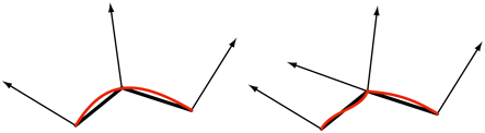
Figure 3.7 Side views of triangle meshes (in black, with vertex normals) representing curved surfaces (in red). On the left smoothed vertex normals are used to represent a smooth surface. On the right the middle vertex has been duplicated and given two normals, representing a crease.
A vertex shader is much the same as the unified shader described earlier. Every vertex passed in is processed by the vertex shader program, which then outputs a number of values that are interpolated across a triangle or line. The vertex shader can neither create nor destroy vertices, and results generated by one vertex cannot be passed on to another vertex. Since each vertex is treated independently, any number of shader processors on the GPU can be applied in parallel to the incoming stream of vertices.
Input assembly is usually presented as a process that happens before the vertex shader is executed. This is an example where the physical model often differs from the logical. Physically, the fetching of data to create a vertex might happen in the vertex shader and the driver will quietly prepend every shader with the appropriate instructions, invisible to the programmer.
Chapters that follow explain several vertex shader effects, such as vertex blending for animating joints, and silhouette rendering. Other uses for the vertex shader include:
- Object generation, by creating a mesh only once and having it be deformed by the vertex shader.
- Animating character’s bodies and faces using skinning and morphing techniques.
- Procedural deformations, such as the movement of flags, cloth, or water [802, 943].
- Particle creation, by sending degenerate (no area) meshes down the pipeline and having these be given an area as needed.
- Lens distortion, heat haze, water ripples, page curls, and other effects, by using the entire framebuffer’s contents as a texture on a screen-aligned mesh undergoing procedural deformation.
- Applying terrain height fields by using vertex texture fetch [40, 1227].
Some deformations done using a vertex shader are shown in Figure 3.8.
The output of the vertex shader can be consumed in several different ways. The usual path is for each instance’s primitives, e.g., triangles, to then be generated and rasterized, and the individual pixel fragments produced to be sent to the pixel shader program for continued processing. On some GPUs the data can also be sent to the tessellation stage or the geometry shader or be stored in memory. These optional stages are discussed in the following sections.

Figure 3.8 On the left, a normal teapot. A simple shear operation performed by a vertex shader program produces the middle image. On the right, a noise function creates a field that distorts the model. (Images produced by FX Composer 2, courtesy of NVIDIA Corporation.)
3.6 The Tessellation Stage
The tessellation stage allows us to render curved surfaces. The GPU’s task is to take each surface description and turn it into a representative set of triangles. This stage is an optional GPU feature that first became available in (and is required by) DirectX 11. It is also supported in OpenGL 4.0 and OpenGL ES 3.2.
There are several advantages to using the tessellation stage. The curved surface description is often more compact than providing the corresponding triangles themselves. Beyond memory savings, this feature can keep the bus between CPU and GPU from becoming the bottleneck for an animated character or object whose shape is changing each frame. The surfaces can be rendered efficiently by having an appropriate number of triangles generated for the given view. For example, if a ball is far from the camera, only a few triangles are needed. Up close, it may look best represented with thousands of triangles. This ability to control the level of detail can also allow an application to control its performance, e.g., using a lower-quality mesh on weaker GPUs in order to maintain frame rate. Models normally represented by flat surfaces can be converted to fine meshes of triangles and then warped as desired [1493], or they can be tessellated in order to perform expensive shading computations less frequently [225].
The tessellation stage always consists of three elements. Using DirectX’s terminology, these are the hull shader, tessellator, and domain shader. In OpenGL the hull shader is the tessellation control shader and the domain shader the tessellation evaluation shader, which are a bit more descriptive, though verbose. The fixed-function tessellator is called the primitive generator in OpenGL, and as will be seen, that is indeed what it does.
How to specify and tessellate curves and surfaces is discussed at length in Chapter 17. Here we give a brief summary of each tessellation stage’s purpose. To begin, the input to the hull shader is a special patch primitive. This consists of several control points defining a subdivision surface, B′ezier patch, or other type of curved element. The hull shader has two functions. First, it tells the tessellator how many triangles should be generated, and in what configuration. Second, it performs processing on each of the control points. Also, optionally, the hull shader can modify the incoming patch description, adding or removing control points as desired. The hull shader outputs its set of control points, along with the tessellation control data, to the domain shader. See Figure 3.9.

Figure 3.9 The tessellation stage. The hull shader takes in a patch de_ned by control points. It sends the tessellation factors (TFs) and type to the _xed-function tessellator. The control point set is transformed as desired by the hull shader and sent on to the domain shader, along with TFs and related patch constants. The tessellator creates the set of vertices along with their barycentric coordinates. These are then processed by the domain shader, producing the triangle mesh (control points shown for reference).
The tessellator is a fixed-function stage in the pipeline, only used with tessellation shaders. It has the task of adding several new vertices for the domain shader to process. The hull shader sends the tessellator information about what type of tessellation surface is desired: triangle, quadrilateral, or isoline. Isolines are sets of line strips, sometimes used for hair rendering [1954]. The other important values sent by the hull shader are the tessellation factors (tessellation levels in OpenGL). These are of two types: inner and outer edge. The two inner factors determine how much tessellation occurs inside the triangle or quadrilateral. The outer factors determine how much each exterior edge is split (Section 17.6). An example of increasing tessellation factors is shown in Figure 3.10. By allowing separate controls, we can have adjacent curved surfaces’ edges match in tessellation, regardless of how the interiors are tessellated. Matching edges avoids cracks or other shading artifacts where patches meet. The vertices are assigned barycentric coordinates (Section 22.8), which are values that specify a relative location for each point on the desired surface.
The hull shader always outputs a patch, a set of control point locations. However, it can signal that a patch is to be discarded by sending the tessellator an outer tessellation level of zero or less (or not-a-number, NaN). Otherwise, the tessellator generates a mesh and sends it to the domain shader. The control points for the curved surface from the hull shader are used by each invocation of the domain shader to compute the output values for each vertex. The domain shader has a data flow pattern like that of a vertex shader, with each input vertex from the tessellator being processed and generating a corresponding output vertex. The triangles formed are then passed on down the pipeline.

Figure 3.10 The effect of varying the tessellation factors. The Utah teapot is made of 32 patches. Inner and outer tessellation factors, from left to right, are 1, 2, 4, and 8. (Images generated by demo from Rideout and Van Gelder [1493].)
While this system sounds complex, it is structured this way for efficiency, and each shader can be fairly simple. The patch passed into a hull shader will often undergo little or no modification. This shader may also use the patch’s estimated distance or screen size to compute tessellation factors on the fly, as for terrain rendering [466]. Alternately, the hull shader may simply pass on a fixed set of values for all patches that the application computes and provides. The tessellator performs an involved but fixed-function process of generating the vertices, giving them positions, and specifying what triangles or lines they form. This data amplification step is performed outside of a shader for computational efficiency [530]. The domain shader takes the barycentric coordinates generated for each point and uses these in the patch’s evaluation equation to generate the position, normal, texture coordinates, and other vertex information desired. See Figure 3.11 for an example.

Figure 3.11 On the left is the underlying mesh of about 6000 triangles. On the right, each triangle is tessellated and displaced using PN triangle subdivision. (Images from NVIDIA SDK 11 [1301] samples, courtesy of NVIDIA Corporation, model from Metro 2033 by 4A Games.)

Figure 3.12 Geometry shader input for a geometry shader program is of some single type: point, line segment, triangle. The two rightmost primitives include vertices adjacent to the line and triangle objects. More elaborate patch types are possible.
3.7 The Geometry Shader
The geometry shader can turn primitives into other primitives, something the tessellation stage cannot do. For example, a triangle mesh could be transformed to a wireframe view by having each triangle create line edges. Alternately, the lines could be replaced by quadrilaterals facing the viewer, so making a wireframe rendering with thicker edges [1492]. The geometry shader was added to the hardware-accelerated graphics pipeline with the release of DirectX 10, in late 2006. It is located after the tessellation shader in the pipeline, and its use is optional. While a required part of Shader Model 4.0, it is not used in earlier shader models. OpenGL 3.2 and OpenGL ES 3.2 support this type of shader as well.
The input to the geometry shader is a single object and its associated vertices. The object typically consists of triangles in a strip, a line segment, or simply a point. Extended primitives can be defined and processed by the geometry shader. In particular, three additional vertices outside of a triangle can be passed in, and the two adjacent vertices on a polyline can be used. See Figure 3.12. With DirectX 11 and Shader Model 5.0, you can pass in more elaborate patches, with up to 32 control points. That said, the tessellation stage is more efficient for patch generation [175].
The geometry shader processes this primitive and outputs zero or more vertices, which are treated as points, polylines, or strips of triangles. Note that no output at all can be generated by the geometry shader. In this way, a mesh can be selectively modified by editing vertices, adding new primitives, and removing others.
The geometry shader is designed for modifying incoming data or making a limited number of copies. For example, one use is to generate six transformed copies of data to simultaneously render the six faces of a cube map; see Section 10.4.3. It can also be used to efficiently create cascaded shadow maps for high-quality shadow generation. Other algorithms that take advantage of the geometry shader include creating variablesized particles from point data, extruding fins along silhouettes for fur rendering, and finding object edges for shadow algorithms. See Figure 3.13 for more examples. These and other uses are discussed throughout the rest of the book.
DirectX 11 added the ability for the geometry shader to use instancing, where the geometry shader can be run a set number of times on any given primitive [530, 1971]. In OpenGL 4.0 this is specified with an invocation count. The geometry shader can also output up to four streams. One stream can be sent on down the rendering pipeline for further processing. All these streams can optionally be sent to stream output render targets.

Figure 3.13 Some uses of the geometry shader (GS). On the left, metaball isosurface tessellation is performed on the fly using the GS. In the middle, fractal subdivision of line segments is done using the GS and stream out, and billboards are generated by the GS for display of the lightning. On the right, cloth simulation is performed by using the vertex and geometry shader with stream out. (Images from NVIDIA SDK 10 [1300] samples, courtesy of NVIDIA Corporation.)
The geometry shader is guaranteed to output results from primitives in the same order that they are input. This affects performance, because if several shader cores run in parallel, results must be saved and ordered. This and other factors work against the geometry shader being used to replicate or create a large amount of geometry in a single call [175, 530].
After a draw call is issued, there are only three places in the pipeline where work can be created on the GPU: rasterization, the tessellation stage, and the geometry shader. Of these, the geometry shader’s behavior is the least predictable when considering resources and memory needed, since it is fully programmable. In practice the geometry shader usually sees little use, as it does not map well to the GPU’s strengths. On some mobile devices it is implemented in software, so its use is actively discouraged there [69].
3.7.1 Stream Output
The standard use of the GPU’s pipeline is to send data through the vertex shader, then rasterize the resulting triangles and process these in the pixel shader. It used to be that the data always passed through the pipeline and intermediate results could not be accessed. The idea of stream output was introduced in Shader Model 4.0. After vertices are processed by the vertex shader (and, optionally, the tessellation and geometry shaders), these can be output in a stream, i.e., an ordered array, in addition to being sent on to the rasterization stage. Rasterization could, in fact, be turned off entirely and the pipeline then used purely as a non-graphical stream processor. Data processed in this way can be sent back through the pipeline, thus allowing iterative processing. This type of operation can be useful for simulating flowing water or other particle effects, as discussed in Section 13.8. It could also be used to skin a model and then have these vertices available for reuse (Section 4.4).
Stream output returns data only in the form of floating point numbers, so it can have a noticeable memory cost. Stream output works on primitives, not directly on vertices. If meshes are sent down the pipeline, each triangle generates its own set of three output vertices. Any vertex sharing in the original mesh is lost. For this reason a more typical use is to send just the vertices through the pipeline as a point set primitive. In OpenGL the stream output stage is called transform feedback, since the focus of much of its use is transforming vertices and returning them for further processing. Primitives are guaranteed to be sent to the stream output target in the order that they were input, meaning the vertex order will be maintained [530].
3.8 The Pixel Shader
After the vertex, tessellation, and geometry shaders perform their operations, the primitive is clipped and set up for rasterization, as explained in the previous chapter. This section of the pipeline is relatively fixed in its processing steps, i.e., not programmable but somewhat configurable. Each triangle is traversed to determine which pixels it covers. The rasterizer may also roughly calculate how much the triangle covers each pixel’s cell area (Section 5.4.2). This piece of a triangle partially or fully overlapping the pixel is called a fragment.
The values at the triangle’s vertices, including the z-value used in the z-buffer, are interpolated across the triangle’s surface for each pixel. These values are passed to the pixel shader, which then processes the fragment. In OpenGL the pixel shader is known as the fragment shader, which is perhaps a better name. We use “pixel shader” throughout this book for consistency. Point and line primitives sent down the pipeline also create fragments for the pixels covered.
The type of interpolation performed across the triangle is specified by the pixel shader program. Normally we use perspective-correct interpolation, so that the worldspace distances between pixel surface locations increase as an object recedes in the distance. An example is rendering railroad tracks extending to the horizon. Railroad ties are more closely spaced where the rails are farther away, as more distance is traveled for each successive pixel approaching the horizon. Other interpolation options are available, such as screen-space interpolation, where perspective projection is not taken into account. DirectX 11 gives further control over when and how interpolation is performed [530].
In programming terms, the vertex shader program’s outputs, interpolated across the triangle (or line), effectively become the pixel shader program’s inputs. As the GPU has evolved, other inputs have been exposed. For example, the screen position of the fragment is available to the pixel shader in Shader Model 3.0 and beyond. Also, which side of a triangle is visible is an input flag. This knowledge is important for rendering a different material on the front versus back of each triangle in a single pass.

Figure 3.14 User-defined clipping planes. On the left, a single horizontal clipping plane slices the object. In the middle, the nested spheres are clipped by three planes. On the right, the spheres’ surfaces are clipped only if they are outside all three clip planes. (From the three.js examples webgl clipping and webgl clipping intersection [218].)
With inputs in hand, typically the pixel shader computes and outputs a fragment’s color. It can also possibly produce an opacity value and optionally modify its z-depth. During merging, these values are used to modify what is stored at the pixel. The depth value generated in the rasterization stage can also be modified by the pixel shader. The stencil buffer value is usually not modifiable, but rather it is passed through to the merge stage. DirectX 11.3 allows the shader to change this value. Operations such as fog computation and alpha testing have moved from being merge operations to being pixel shader computations in SM 4.0 [175].
A pixel shader also has the unique ability to discard an incoming fragment, i.e., generate no output. One example of how fragment discard can be used is shown in Figure 3.14. Clip plane functionality used to be a configurable element in the fixedfunction pipeline and was later specified in the vertex shader. With fragment discard available, this functionality could then be implemented in any way desired in the pixel shader, such as deciding whether clipping volumes should be AND’ed or OR’ed together.
Initially the pixel shader could output to only the merging stage, for eventual display. The number of instructions a pixel shader can execute has grown considerably over time. This increase gave rise to the idea of multiple render targets (MRT). Instead of sending results of a pixel shader’s program to just the color and z-buffer, multiple sets of values could be generated for each fragment and saved to different buffers, each called a render target. Render targets generally have the same xand y-dimensions; some APIs allow different sizes, but the rendered area will be the smallest of these. Some architectures require render targets to each have the same bit depth, and possibly even identical data formats. Depending on the GPU, the number of render targets available is four or eight.
Even with these limitations, MRT functionality is a powerful aid in performing rendering algorithms more efficiently. A single rendering pass could generate a color image in one target, object identifiers in another, and world-space distances in a third. This ability has also given rise to a different type of rendering pipeline, called deferred shading, where visibility and shading are done in separate passes. The first pass stores data about an object’s location and material at each pixel. Successive passes can then efficiently apply illumination and other effects. This class of rendering methods is described in Section 20.1.
The pixel shader’s limitation is that it can normally write to a render target at only the fragment location handed to it, and cannot read current results from neighboring pixels. That is, when a pixel shader program executes, it cannot send its output directly to neighboring pixels, nor can it access others’ recent changes. Rather, it computes results that affect only its own pixel. However, this limitation is not as severe as it sounds. An output image created in one pass can have any of its data accessed by a pixel shader in a later pass. Neighboring pixels can be processed using image processing techniques, described in Section 12.1.
There are exceptions to the rule that a pixel shader cannot know or affect neighboring pixels’ results. One is that the pixel shader can immediately access information for adjacent fragments (albeit indirectly) during the computation of gradient or derivative information. The pixel shader is provided with the amounts by which any interpolated value changes per pixel along the x and y screen axes. Such values are useful for various computations and texture addressing. These gradients are particularly important for operations such as texture filtering (Section 6.2.2), where we want to know how much of an image covers a pixel. All modern GPUs implement this feature by processing fragments in groups of 2 × 2, called a quad. When the pixel shader requests a gradient value, the difference between adjacent fragments is returned. See Figure 3.15. A unified core has this capability to access neighboring data—kept in different threads on the same warp—and so can compute gradients for use in the pixel shader. One consequence of this implementation is that gradient information cannot be accessed in parts of the shader affected by dynamic flow control, i.e., an “if” statement or loop with a variable number of iterations. All the fragments in a group must be processed using the same set of instructions so that all four pixels’ results are meaningful for computing gradients. This is a fundamental limitation that exists even in offline rendering systems [64].
DirectX 11 introduced a buffer type that allows write access to any location, the unordered access view (UAV). Originally for only pixel and compute shaders, access to UAVs was extended to all shaders in DirectX 11.1 [146]. OpenGL 4.3 calls this a shader storage buffer object (SSBO). Both names are descriptive in their own way. Pixel shaders are run in parallel, in an arbitrary order, and this storage buffer is shared among them.
Often some mechanism is needed to avoid a data race condition (a.k.a. a data hazard), where both shader programs are “racing” to influence the same value, possibly leading to arbitrary results. As an example, an error could occur if two invocations of a pixel shader tried to, say, add to the same retrieved value at about the same time. Both would retrieve the original value, both would modify it locally, but then whichever invocation wrote its result last would wipe out the contribution of the other invocation—only one addition would occur. GPUs avoid this problem by having dedicated atomic units that the shader can access [530]. However, atomics mean that some shaders may stall as they wait to access a memory location undergoing read/modify/write by another shader.

Figure 3.15 On the left, a triangle is rasterized into quads, sets of 2 × 2 pixels. The gradient computations for the pixel marked with a black dot is then shown on the right. The value for v is shown for each of the four pixel locations in the quad. Note how three of the pixels are not covered by the triangle, yet they are still processed by the GPU so that the gradients can be found. The gradients in the x and y screen directions are computed for the lower left pixel by using its two quad neighbors.
While atomics avoid data hazards, many algorithms require a specific order of execution. For example, you may want to draw a more distant transparent blue triangle before overlaying it with a red transparent triangle, blending the red atop the blue. It is possible for a pixel to have two pixel shader invocations for a pixel, one for each triangle, executing in such a way that the red triangle’s shader completes before the blue’s. In the standard pipeline, the fragment results are sorted in the merger stage before being processed. Rasterizer order views (ROVs) were introduced in DirectX 11.3 to enforce an order of execution. These are like UAVs; they can be read and written by shaders in the same fashion. The key difference is that ROVs guarantee that the data are accessed in the proper order. This increases the usefulness of these shader-accessible buffers considerably [327, 328]. For example, ROVs make it possible for the pixel shader to write its own blending methods, since it can directly access and write to any location in the ROV, and thus no merging stage is needed [176]. The price is that, if an out-of-order access is detected, a pixel shader invocation may stall until triangles drawn earlier are processed.
3.9 The Merging Stage
As discussed in Section 2.5.2, the merging stage is where the depths and colors of the individual fragments (generated in the pixel shader) are combined with the framebuffer. DirectX calls this stage the output merger; OpenGL refers to it as per-sample operations. On most traditional pipeline diagrams (including our own), this stage is where stencil-buffer and z-buffer operations occur. If the fragment is visible, another operation that takes place in this stage is color blending. For opaque surfaces there is no real blending involved, as the fragment’s color simply replaces the previously stored color. Actual blending of the fragment and stored color is commonly used for transparency and compositing operations (Section 5.5).
Imagine that a fragment generated by rasterization is run through the pixel shader and then is found to be hidden by some previously rendered fragment when the zbuffer is applied. All the processing done in the pixel shader was then unnecessary. To avoid this waste, many GPUs perform some merge testing before the pixel shader is executed [530]. The fragment’s z-depth (and whatever else is in use, such as the stencil buffer or scissoring) is used for testing visibility. The fragment is culled if hidden. This functionality is called early-z [1220, 1542]. The pixel shader has the ability to change the z-depth of the fragment or to discard the fragment entirely. If either type of operation is found to exist in a pixel shader program, early-z then generally cannot be used and is turned off, usually making the pipeline less efficient. DirectX 11 and OpenGL 4.2 allow the pixel shader to force early-z testing to be on, though with a number of limitations [530]. See Section 23.7 for more about early-z and other z-buffer optimizations. Using early-z effectively can have a large effect on performance, which is discussed in detail in Section 18.4.5.
The merging stage occupies the middle ground between fixed-function stages, such as triangle setup, and the fully programmable shader stages. Although it is not programmable, its operation is highly configurable. Color blending in particular can be set up to perform a large number of different operations. The most common are combinations of multiplication, addition, and subtraction involving the color and alpha values, but other operations are possible, such as minimum and maximum, as well as bitwise logic operations. DirectX 10 added the capability to blend two colors from the pixel shader with the framebuffer color. This capability is called dual source-color blending and cannot be used in conjunction with multiple render targets. MRT does otherwise support blending, and DirectX 10.1 introduced the capability to perform different blend operations on each separate buffer.
As mentioned at the end of the previous section, DirectX 11.3 provided a way to make blending programmable through ROVs, though at a price in performance. ROVs and the merging stage both guarantee draw order, a.k.a. output invariance. Regardless of the order in which pixel shader results are generated, it is an API requirement that results are sorted and sent to the merging stage in the order in which they are input, object by object and triangle by triangle.
3.10 The Compute Shader
The GPU can be used for more than implementing the traditional graphics pipeline. There are many non-graphical uses in fields as varied as computing the estimated value of stock options and training neural nets for deep learning. Using hardware in this way is called GPU computing. Platforms such as CUDA and OpenCL are used to control the GPU as a massive parallel processor, with no real need or access to graphics-specific functionality. These frameworks often use languages such as C or C++ with extensions, along with libraries made for the GPU.
Introduced in DirectX 11, the compute shader is a form of GPU computing, in that it is a shader that is not locked into a location in the graphics pipeline. It is closely tied to the process of rendering in that it is invoked by the graphics API. It is used alongside vertex, pixel, and other shaders. It draws upon the same pool of unified shader processors as those used in the pipeline. It is a shader like the others, in that it has some set of input data and can access buffers (such as textures) for input and output. Warps and threads are more visible in a compute shader. For example, each invocation gets a thread index that it can access. There is also the concept of a thread group, which consists of 1 to 1024 threads in DirectX 11. These thread groups are specified by x-, y-, and z-coordinates, mostly for simplicity of use in shader code. Each thread group has a small amount of memory that is shared among threads. In DirectX 11, this amounts to 32 kB. Compute shaders are executed by thread group, so that all threads in the group are guaranteed to run concurrently [1971].
One important advantage of compute shaders is that they can access data generated on the GPU. Sending data from the GPU to the CPU incurs a delay, so performance can be improved if processing and results can be kept resident on the GPU [1403]. Post-processing, where a rendered image is modified in some way, is a common use of compute shaders. The shared memory means that intermediate results from sampling image pixels can be shared with neighboring threads. Using a compute shader to determine the distribution or average luminance of an image, for example, has been found to run twice as fast as performing this operation on a pixel shader [530].
Compute shaders are also useful for particle systems, mesh processing such as facial animation [134], culling [1883, 1884], image filtering [1102, 1710], improving depth precision [991], shadows [865], depth of field [764], and any other tasks where a set of GPU processors can be brought to bear. Wihlidal [1884] discusses how compute shaders can be more efficient than tessellation hull shaders. See Figure 3.16 for other uses.
This ends our review of the GPU’s implementation of the rendering pipeline. There are many ways in which the GPUs functions can be used and combined to perform various rendering-related processes. Relevant theory and algorithms tuned to take advantage of these capabilities are the central subjects of this book. Our focus now moves on to transforms and shading.

Figure 3.16 Compute shader examples. On the left, a compute shader is used to simulate hair affected by wind, with the hair itself rendered using the tessellation stage. In the middle, a compute shader performs a rapid blur operation. On the right, ocean waves are simulated. (Images from NVIDIA SDK 11 [1301] samples, courtesy of NVIDIA Corporation.)
Further Reading and Resources
Giesen’s tour of the graphics pipeline [530] discusses many facets of the GPU at length, explaining why elements work the way they do. The course by Fatahalian and Bryant [462] discusses GPU parallelism in a series of detailed lecture slide sets. While focused on GPU computing using CUDA, the introductory part of Kirk and Hwa’s book [903] discusses the evolution and design philosophy for the GPU.
To learn the formal aspects of shader programming takes some work. Books such as the OpenGL Superbible [1606] and OpenGL Programming Guide [885] include material on shader programming. The older book OpenGL Shading Language [1512] does not cover more recent shader stages, such as the geometry and tessellation shaders, but does focus specifically on shader-related algorithms. See this book’s website, realtimerendering.com, for recent and recommended books.