
Chapter 4
Transforms
“What if angry vectors veer
Round your sleeping head, and form.
There’s never need to fear
Violence of the poor world’s abstract storm.”
—Robert Penn Warren
A transform is an operation that takes entities such as points, vectors, or colors and converts them in some way. For the computer graphics practitioner, it is extremely important to master transforms. With them, you can position, reshape, and animate objects, lights, and cameras. You can also ensure that all computations are carried out in the same coordinate system, and project objects onto a plane in different ways. These are only a few of the operations that can be performed with transforms, but they are sufficient to demonstrate the importance of the transform’s role in real-time graphics, or, for that matter, in any kind of computer graphics.
A linear transform is one that preserves vector addition and scalar multiplication. Specifically,
(4.1)
f(x)+f(y)=f(x+y),(4.2)
kf(x)=f(kx).As an example, f(x)=5x
However, this size of matrix is usually not large enough. A function for a three-element vector x such as f(x)=x+(7,3,2)
Combining linear transforms and translations can be done using an affine transform, typically stored as a 4×4
All translation, rotation, scaling, reflection, and shearing matrices are affine. The main characteristic of an affine matrix is that it preserves the parallelism of lines, but not necessarily lengths and angles. An affine transform may also be any sequence of concatenations of individual affine transforms.
This chapter will begin with the most essential, basic affine transforms. This section can be seen as a “reference manual” for simple transforms. More specialized matrices are then described, followed by a discussion and description of quaternions, a powerful transform tool. Then follows vertex blending and morphing, which are two simple but effective ways of expressing animations of meshes. Finally, projection matrices are described. Most of these transforms, their notations, functions, and properties are summarized in Table 4.1, where an orthogonal matrix is one whose inverse is the transpose.
Transforms are a basic tool for manipulating geometry. Most graphics application programming interfaces let the user set arbitrary matrices, and sometimes a library may be used with matrix operations that implement many of the transforms discussed in this chapter. However, it is still worthwhile to understand the real matrices and their interaction behind the function calls. Knowing what the matrix does after such a function call is a start, but understanding the properties of the matrix itself will take you further. For example, such an understanding enables you to discern when you are dealing with an orthogonal matrix, whose inverse is its transpose, making for faster matrix inversions. Knowledge like this can lead to accelerated code.
4.1 Basic Transforms
This section describes the most basic transforms, such as translation, rotation, scaling, shearing, transform concatenation, the rigid-body transform, normal transform (which is not so normal), and computation of inverses. For the experienced reader, this can be used as a reference manual for simple transforms, and for the novice, it can serve as an introduction to the subject. This material is necessary background for the rest of this chapter and for other chapters in this book. We start with the simplest of transforms—the translation.
Table 4.1. Summary of most of the transforms discussed in this chapter.

4.1.1. Translation
A change from one location to another is represented by a translation matrix, T
(4.3)
T(t)=T(tx,ty,tz)=(100tx010ty001tz0001).An example of the effect of the translation transform is shown in Figure 4.1. It is easily shown that the multiplication of a point p=(px,py,pz,1)

Figure 4.1. The square on the left is transformed with a translation matrix T(5, 2, 0), whereby the square is moved 5 distance units to the right and 2 upward.
We should mention at this point that another valid notational scheme sometimes seen in computer graphics uses matrices with translation vectors in the bottom row. For example, DirectX uses this form. In this scheme, the order of matrices would be reversed, i.e., the order of application would read from left to right. Vectors and matrices in this notation are said to be in row-major form since the vectors are rows. In this book, we use column-major form. Whichever is used, this is purely a notational difference. When the matrix is stored in memory, the last four values of the sixteen are the three translation values followed by a one.
4.1.2. Rotation
A rotation transform rotates a vector (position or direction) by a given angle around a given axis passing through the origin. Like a translation matrix, it is a rigid-body transform, i.e., it preserves the distances between points transformed, and preserves handedness (i.e., it never causes left and right to swap sides). These two types of transforms are clearly useful in computer graphics for positioning and orienting objects. An orientation matrix is a rotation matrix associated with a camera view or object that defines its orientation in space, i.e., its directions for up and forward.
In two dimensions, the rotation matrix is simple to derive. Assume that we have a vector, v=(vx,vy)
(4.4)
u=(rcos(θ+ϕ)rsin(θ+ϕ))=(r(cosθcosϕ-sinθsinϕ)r(sinθcosϕ+cosθsinϕ))=(cosϕ-sinϕsinϕcosϕ)⏟R(ϕ)(rcosθrsinθ)⏟v=R(ϕ)v,where we used the angle sum relation to expand cos(θ+ϕ) and sin(θ+ϕ) . In three dimensions, commonly used rotation matrices are Rx(ϕ) , Ry(ϕ) , and Rz(ϕ) , which rotate an entity ϕ radians around the x-, y-, and z-axes, respectively. They are given by Equations 4.5–4.7:
(4.5)
Rx(ϕ)=(10000cosϕ-sinϕ00sinϕcosϕ00001),(4.6)
Ry(ϕ)=(cosϕ0sinϕ00100-sinϕ0cosϕ00001),(4.7)
Rz(ϕ)=(cosϕ-sinϕ00sinϕcosϕ0000100001).If the bottom row and rightmost column are deleted from a 4×4 matrix, a 3×3 matrix is obtained. For every 3×3 rotation matrix, R, that rotates ϕ radians around is constant independent of the axis, and is computed as [997]:
(4.8)
tr(R)=1+2cosϕ.The effect of a rotation matrix may be seen in Figure 4.4 on page 65. What characterizes a rotation matrix, Ri(ϕ) , besides the fact that it rotates ϕ radians around axis i, is that it leaves all points on the rotation axis, i, unchanged. Note that R will also be used to denote a rotation matrix around any axis. The axis rotation matrices given above can be used in a series of three transforms to perform any arbitrary axis rotation. This procedure is discussed in Section 4.2.1. Performing a rotation around an arbitrary axis directly is covered in Section 4.2.4.
All rotation matrices have a determinant of one and are orthogonal. This also holds for concatenations of any number of these transforms. There is another way to obtain the inverse: R-1i(ϕ)=Ri(-ϕ) , i.e., rotate in the opposite direction around the same axis.
EXAMPLE: ROTATION AROUND A POINT. Assume that we want to rotate an object by ϕ radians around the z-axis, with the center of rotation being a certain point, p. What is the transform? This scenario is depicted in Figure 4.2. Since a rotation around a point is characterized by the fact that the point itself is unaffected by the rotation, the transform starts by translating the object so that p coincides with the origin, which is done with T(-p) . Thereafter follows the actual rotation: Rz(ϕ) . Finally, the object has to be translated back to its original position using T( p). The resulting transform, X, is then given by
(4.9)
X=T(p)Rz(ϕ)T(-p).Note the order of the matrices above.

Figure 4.2. Example of rotation around a specific point p.
4.1.3. Scaling
A scaling matrix, S(s)=S(sx,sy,sz) , scales an entity with factors sx , sy , and sz along the x-, y-, and z-directions, respectively. This means that a scaling matrix can be used to enlarge or diminish an object. The larger the si , i∈{x,y,z} , the larger the scaled entity gets in that direction. Setting any of the components of s to 1 naturally avoids a change in scaling in that direction. Equation 4.10 shows S :
(4.10)
S(s)=(sx0000sy0000sz00001).Figure 4.4 on page 65 illustrates the effect of a scaling matrix. The scaling operation is called uniform if sx=sy=sz and nonuniform otherwise. Sometimes the terms isotropic and anisotropic scaling are used instead of uniform and nonuniform. The inverse is S-1(s)=S(1/sx,1/sy,1/sz) .
Using homogeneous coordinates, another valid way to create a uniform scaling matrix is by manipulating matrix element at position (3, 3), i.e., the element at the lower right corner. This value affects the w-component of the homogeneous coordinate, and so scales every coordinate of a point (not direction vectors) transformed by the matrix. For example, to scale uniformly by a factor of 5, the elements at (0, 0), (1, 1), and (2, 2) in the scaling matrix can be set to 5, or the element at (3, 3) can be set to 1 / 5. The two different matrices for performing this are shown below:
(4.11)
S=(5000050000500001),S′=(1000010000100001/5).In contrast to using S for uniform scaling, using S′ must always be followed by homogenization. This may be inefficient, since it involves divides in the homogenization process; if the element at the lower right (position (3, 3)) is 1, no divides are necessary. Of course, if the system always does this division without testing for 1, then there is no extra cost.
A negative value on one or three of the components of s gives a type of reflection matrix, also called a mirror matrix. If only two scale factors are -1 , then we will rotate π radians. It should be noted that a rotation matrix concatenated with a reflection matrix is also a reflection matrix. Hence, the following is a reflection matrix:
(4.12)
(cos(π/2)sin(π/2)-sin(π/2)cos(π/2))⏟rotation(100-1)⏟reflection=(0-1-10).Reflection matrices usually require special treatment when detected. For example, a triangle with vertices in a counterclockwise order will get a clockwise order when transformed by a reflection matrix. This order change can cause incorrect lighting and backface culling to occur. To detect whether a given matrix reflects in some manner, compute the determinant of the upper left 3×3 elements of the matrix. If the value is negative, the matrix is reflective. For example, the determinant of the matrix in Equation 4.12 is 0·0-(-1)·(-1)=-1 .
EXAMPLE: SCALING IN A CERTAIN DIRECTION. The scaling matrix S scales along only the x-, y-, and z-axes. If scaling should be performed in other directions, a compound transform is needed. Assume that scaling should be done along the axes of the orthonormal, right-oriented vectors fx , fy , and fz . First, construct the matrix F, to change the basis, as below:
(4.13)
F=(fxfyfz00001).The idea is to make the coordinate system given by the three axes coincide with the standard axes, then use the standard scaling matrix, and then transform back. The first step is carried out by multiplying with the transpose, i.e., the inverse, of F. Then the actual scaling is done, followed by a transform back. The transform is shown in Equation 4.14:
(4.14)
X=FS(s)FT.4.1.4. Shearing
Another class of transforms is the set of shearing matrices. These can, for example, be used in games to distort an entire scene to create a psychedelic effect or otherwise warp a model’s appearance. There are six basic shearing matrices, and they are denoted Hxy(s) , Hxz(s) , Hyx(s) , Hyz(s) , Hzx(s) , and Hzy(s) . The first subscript is used to denote which coordinate is being changed by the shear matrix, while the second subscript indicates the coordinate which does the shearing. An example of a shear matrix, Hxz(s) , is shown in Equation 4.15. Observe that the subscript can be used to find the position of the parameter s in the matrix below; the x (whose numeric index is 0) identifies row zero, and the z (whose numeric index is 2) identifies column two, and so the s is located there:

Figure 4.3. The effect of shearing the unit square with Hxz(s) . Both the y- and z-values are unaffected by the transform, while the x-value is the sum of the old x-value and s multiplied by the z-value, causing the square to become slanted. This transform is area-preserving, which can be seen in that the dashed areas are the same.
(4.15)
Hxz(s)=(10s0010000100001).The effect of multiplying this matrix with a point p yields a point: (px+spzpypz)T . Graphically, this is shown for the unit square in Figure 4.3.
The inverse of Hij(s) (shearing the ith coordinate with respect to the jth coordinate, where i≠j ), is generated by shearing in the opposite direction, that is, H-1ij(s)=Hij(-s) .
You can also use a slightly different kind of shear matrix:
(4.16)
H′xy(s,t)=(10s001t000100001).Here, however, both subscripts are used to denote that these coordinates are to be sheared by the third coordinate. The connection between these two different kinds of descriptions is H′ij(s,t)=Hik(s)Hjk(t) , where k is used as an index to the third coordinate. The right matrix to use is a matter of taste. Finally, it should be noted that since the determinant of any shear matrix |H|=1 , this is a volume-preserving transformation, which also is illustrated in Figure 4.3.
4.1.5. Concatenation of Transforms
Due to the noncommutativity of the multiplication operation on matrices, the order in which the matrices occur matters. Concatenation of transforms is therefore said to be order-dependent.
As an example of order dependency, consider two matrices, S and R. S(2, 0.5, 1) scales the x-component by a factor two and the y-component by a factor 0.5. Rz(π/6) rotates π/6 radians counterclockwise around the z-axis (which points outward from page of this book in a right-handed coordinate system). These matrices can be multiplied in two ways, with the results being entirely different. The two cases are shown in Figure 4.4.
The obvious reason to concatenate a sequence of matrices into a single one is to gain efficiency. For example, imagine that you have a game scene that has several million vertices, and that all objects in the scene must be scaled, rotated, and finally translated. Now, instead of multiplying all vertices with each of the three matrices, the three matrices are concatenated into a single matrix. This single matrix is then applied to the vertices. This composite matrix is C=TRS . Note the order here. The scaling matrix, S, should be applied to the vertices first, and therefore appears to the right in the composition. This ordering implies that TRSp=(T(R(Sp))) , where p is a point to be transformed. Incidentally, T R S is the order commonly used by scene graph systems.
It is worth noting that while matrix concatenation is order-dependent, the matrices can be grouped as desired. For example, say that with T R S p you would like to compute the rigid-body motion transform T R once. It is valid to group these two matrices together, ( T R)( S p), and replace with the intermediate result. Thus, matrix concatenation is associative.
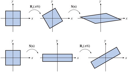
Figure 4.4. This illustrates the order dependency when multiplying matrices. In the top row, the rotation matrix Rz(π/6) is applied followed by a scaling, S( s), where s=(2,0.5,1) . The composite matrix is then S(s)Rz(π/6) . In the bottom row, the matrices are applied in the reverse order, yielding Rz(π/6)S(s) . The results are clearly different. It generally holds that MN≠NM , for arbitrary matrices M and N.
4.1.6. The Rigid-Body Transform
When a person grabs a solid object, say a pen from a table, and moves it to another location, perhaps to a shirt pocket, only the object’s orientation and location change, while the shape of the object generally is not affected. Such a transform, consisting of concatenations of only translations and rotations, is called a rigid-body transform. It has the characteristic of preserving lengths, angles, and handedness.
Any rigid-body matrix, X , can be written as the concatenation of a translation matrix, T(t) , and a rotation matrix, R . Thus, X has the appearance of the matrix in Equation 4.17:
(4.17)
X=T(t)R=(r00r01r02txr10r11r12tyr20r21r22tz0001).The inverse of X is computed as X-1=(T(t)R)-1=R-1T(t)-1=RTT(-t) . Thus, to compute the inverse, the upper left 3×3 matrix of R is transposed, and the translation values of T change sign. These two new matrices are multiplied together in opposite order to obtain the inverse. Another way to compute the inverse of X is to consider R (making R appear as 3×3 matrix) and X in the following notation (notation described on page 6 with Equation ):
(4.18)
ˉR=(r,0r,1r,2)=(rT0,[9pt]rT1,[9pt]rT2,),[12pt]⟹X=(ˉRt0T1),where r,0 means the first column of the rotation matrix (i.e., the comma indicates any value from 0 to 2, while the second subscript is 0) and rT0, is the first row of the column matrix. Note that 0 is a 3×1 column vector filled with zeros. Some calculations yield the inverse in the expression shown in Equation 4.19:
(4.19)
X-1=(r0,r1,r2,-ˉRTt0001).
Figure 4.5. The geometry involved in computing a transform that orients the camera at c, with up vector u′ , to look at the point l. For that purpose, we need to compute r, u, and v.
EXAMPLE: ORIENTING THE CAMERA. A common task in graphics is to orient the camera so that it looks at a certain position. Here we will present what gluLookAt() (from the OpenGL Utility Library, GLU for short) does. Even though this function call itself is not used much nowadays, the task remains common. Assume that the camera is located at c, that we want the camera to look at a target l, and that a given up direction of the camera is u′ , as illustrated in Figure 4.5. We want to compute a basis consisting of three vectors, {r,u,v} . We start by computing the view vector as v=(c-l)/||c-l|| , i.e., the normalized vector from the target to the camera position. A vector looking to the “right” can then be computed as r=-(v×u′)/||v×u′|| . The u′ vector is often not guaranteed to be pointing precisely up, so the final up vector is another cross product, u=v×r , which is guaranteed to be normalized since both v and r are normalized and perpendicular by construction. In the camera transform matrix, M, that we will construct, the idea is to first translate everything so the camera position is at the origin, (0, 0, 0), and then change the basis so that r is aligned with (1, 0, 0), u with (0, 1, 0), and v with (0, 0, 1). This is done by
(4.20)
M=(rxryrz0uxuyuz0vxvyvz00001)⏟change of basis(100-tx010-ty001-tz0001)⏟translation=(rxryrz-t·ruxuyuz-t·uvxvyvz-t·v0001).Note that when concatenating the translation matrix with the change of basis matrix, the translation -t is to the right since it should be applied first. One way to remember where to put the components of r, u, and v is the following. We want r to become (1, 0, 0), so when multiplying a change of basis matrix with (1, 0, 0), we can see that the first row in the matrix must be the elements of r, since r·r=1 . Furthermore, the second row and the third row must consist of vectors that are perpendicular to r, i.e., r·x=0 . When applying the same thinking also to u and v, we arrive at the change of basis matrix above.

Figure 4.6. On the left is the original geometry, a triangle and its normal shown from the side. The middle illustration shows what happens if the model is scaled along the x- axis by 0.5 and the normal uses the same matrix. The right figure shows the proper transform of the normal.
4.1.7. Normal Transform
A single matrix can be used to consistently transform points, lines, triangles, and other geometry. The same matrix can also transform tangent vectors following along these lines or on the surfaces of triangles. However, this matrix cannot always be used to transform one important geometric property, the surface normal (and the vertex lighting normal). Figure 4.6 shows what can happen if this same matrix is used.
Instead of multiplying by the matrix itself, the proper method is to use the transpose of the matrix’s adjoint [227]. Computation of the adjoint is described in our online linear algebra appendix. The adjoint is always guaranteed to exist. The normal is not guaranteed to be of unit length after being transformed, so typically needs to be normalized.
The traditional answer for transforming the normal is that the transpose of the inverse is computed [1794]. This method normally works. The full inverse is not necessary, however, and occasionally cannot be created. The inverse is the adjoint divided by the original matrix’s determinant. If this determinant is zero, the matrix is singular, and the inverse does not exist.
Even computing just the adjoint for a full 4×4 matrix can be expensive, and is usually not necessary. Since the normal is a vector, translation will not affect it. Furthermore, most modeling transforms are affine. They do not change the w-component of the homogeneous coordinate passed in, i.e., they do not perform projection. Under these (common) circumstances, all that is needed for normal transformation is to compute the adjoint of the upper left 3×3 components.
Often even this adjoint computation is not needed. Say we know the transform matrix is composed entirely of a concatenation of translations, rotations, and uniform scaling operations (no stretching or squashing). Translations do not affect the normal. The uniform scaling factors simply change the length of the normal. What is left is a series of rotations, which always yields a net rotation of some sort, nothing more. The transpose of the inverse can be used to transform normals. A rotation matrix is defined by the fact that its transpose is its inverse. Substituting to get the normal transform, two transposes (or two inverses) give the original rotation matrix. Putting it all together, the original transform itself can also be used directly to transform normals under these circumstances.
Finally, fully renormalizing the normal produced is not always necessary. If only translations and rotations are concatenated together, the normal will not change length when transformed by the matrix, so no renormalizing is needed. If uniform scalings are also concatenated, the overall scale factor (if known, or extracted—Section 4.2.3) can be used to directly normalize the normals produced. For example, if we know that a series of scalings were applied that makes the object 5.2 times larger, then normals transformed directly by this matrix are renormalized by dividing them by 5.2. Alternately, to create a normal transform matrix that would produce normalized results, the original matrix’s 3×3 upper left could be divided by this scale factor once.
Note that normal transforms are not an issue in systems where, after transformation, the surface normal is derived from the triangle (e.g., using the cross product of the triangle’s edges). Tangent vectors are different than normals in nature, and are always directly transformed by the original matrix.
4.1.8. Computation of Inverses
Inverses are needed in many cases, for example, when changing back and forth between coordinate systems. Depending on the available information about a transform, one of the following three methods of computing the inverse of a matrix can be used:
- If the matrix is a single transform or a sequence of simple transforms with given parameters, then the matrix can be computed easily by “inverting the parameters” and the matrix order. For example, if M=T(t)R(ϕ) , then M-1=R(-ϕ)T(-t) . This is simple and preserves the accuracy of the transform, which is important when rendering huge worlds [1381].
- If the matrix is known to be orthogonal, then M-1=MT , i.e., the transpose is the inverse. Any sequence of rotations is a rotation, and so is orthogonal.
- If nothing is known, then the adjoint method, Cramer’s rule, LU decomposition, or Gaussian elimination could be used to compute the inverse. Cramer’s rule and the adjoint method are generally preferable, as they have fewer branch operations; “if” tests are good to avoid on modern architectures. See Section 4.1.7 on how to use the adjoint to invert transform normals.
The purpose of the inverse computation can also be taken into account when optimizing. For example, if the inverse is to be used for transforming vectors, then only the 3×3 upper left part of the matrix normally needs to be inverted (see the previous section).
4.2 Special Matrix Transforms and Operations
In this section, several matrix transforms and operations that are essential to real-time graphics will be introduced and derived. First, we present the Euler transform (along with its extraction of parameters), which is an intuitive way to describe orientations. Then we touch upon retrieving a set of basic transforms from a single matrix. Finally, a method is derived that rotates an entity around an arbitrary axis.
4.2.1. The Euler Transform
This transform is an intuitive way to construct a matrix to orient yourself (i.e., the camera) or any other entity in a certain direction. Its name comes from the great Swiss mathematician Leonhard Euler (1707–1783).
First, some kind of default view direction must be established. Most often it lies along the negative z-axis with the head oriented along the y-axis, as depicted in Figure 4.7.
The Euler transform is the multiplication of three matrices, namely the rotations shown in the figure. More formally, the transform, denoted E , is given by Equation 4.21:
(4.21)
E(h,p,r)=Rz(r)Rx(p)Ry(h).The order of the matrices can be chosen in 24 different ways [1636]; we present this one because it is commonly used. Since E is a concatenation of rotations, it is also clearly orthogonal. Therefore its inverse can be expressed as E-1=ET=(RzRxRy)T=RTyRTxRTz , although it is, of course, easier to use the transpose of E directly.
The Euler angles h, p, and r represent in which order and how much the head, pitch, and roll should rotate around their respective axes. Sometimes the angles are all called “rolls,” e.g., our “head” is the “y-roll” and our “pitch” is the “x-roll.” Also, “head” is sometimes known as “yaw,” such as in flight simulation.
This transform is intuitive and therefore easy to discuss in layperson’s language. For example, changing the head angle makes the viewer shake their head “no,” changing the pitch makes them nod, and rolling makes them tilt their head sideways. Rather than talking about rotations around the x-, y-, and z-axes, we talk about altering the head, pitch, and roll. Note that this transform can orient not only the camera, but also any object or entity as well. These transforms can be performed using the global axes of the world space or relative to a local frame of reference.
It is important to note that some presentations of Euler angles give the z-axis as the initial up direction. This difference is purely a notational change, though a potentially confusing one. In computer graphics there is a division in how the world is regarded and thus how content is formed: y-up or z-up. Most manufacturing processes, including 3D printing, consider the z-direction to be up in world space; aviation and sea vehicles consider -z to be up. Architecture and GIS normally use z-up, as a building plan or map is two-dimensional, x and y. Media-related modeling systems often consider the y-direction as up in world coordinates, matching how we always describe a camera’s screen up direction in computer graphics. The difference between these two world up vector choices is just a 90∘ rotation (and possibly a reflection) away, but not knowing which is assumed can lead to problems. In this volume we use a world direction of y-up unless otherwise noted.

Figure 4.7. The Euler transform and how it relates to the way you change the head, pitch, and roll angles. The default view direction is shown, looking along the negative z-axis with the up direction along the y-axis.
We also want to point out that the camera’s up direction in its view space has nothing in particular to do with the world’s up direction. Roll your head and the view is tilted, with its world-space up direction differing from the world’s. As another example, say the world uses y-up and our camera looks straight down at the terrain below, a bird’s eye view. This orientation means the camera has pitched 90∘ forward, so that its up direction in world space is (0,0,-1) . In this orientation the camera has no y-component and instead considers -z to be up in world space, but “y is up” remains true in view space, by definition.
While useful for small angle changes or viewer orientation, Euler angles have some other serious limitations. It is difficult to work with two sets of Euler angles in combination. For example, interpolation between one set and another is not a simple matter of interpolating each angle. In fact, two different sets of Euler angles can give the same orientation, so any interpolation should not rotate the object at all. These are some of the reasons that using alternate orientation representations such as quaternions, discussed later in this chapter, are worth pursuing. With Euler angles, you can also get something called gimbal lock, which will be explained next in Section 4.2.2.
4.2.2. Extracting Parameters from the Euler Transform
In some situations, it is useful to have a procedure that extracts the Euler parameters, h, p, and r, from an orthogonal matrix. This procedure is shown in Equation 4.22:
(4.22)
E(h,p,r)=(e00e01e02e10e11e12e20e21e22)=Rz(r)Rx(p)Ry(h).Here we abandoned the 4×4 matrices for 3×3 matrices, since the latter provide all the necessary information for a rotation matrix. That is, the rest of the equivalent 4×4 matrix always contains zeros and a one in the lower right position.
Concatenating the three rotation matrices in Equation 4.22 yields
(4.23)
E=(cosrcosh-sinrsinpsinh-sinrcospcosrsinh+sinrsinpcoshsinrcosh+cosrsinpsinhcosrcospsinrsinh-cosrsinpcosh-cospsinhsinpcospcosh).From this it is apparent that the pitch parameter is given by sinp=e21 . Also, dividing e01 by e11 , and similarly dividing e20 by e22 , gives rise to the following extraction equations for the head and roll parameters:
(4.24)
e01e11=-sinrcosr=-tanrande20e22=-sinhcosh=-tanh.Thus, the Euler parameters h (head), p (pitch), and r (roll) are extracted from a matrix E using the function atan2(y,x) (see page 8 in Chapter 1) as in Equation 4.25:
(4.25)
h=atan2(-e20,e22),p=arcsin(e21),r=atan2(-e01,e11).However, there is a special case we need to handle. If cosp=0 , we have gimbal lock (Section 4.2.2) and rotation angles r and h will rotate around the same axis (though possibly in different directions, depending on whether the p rotation angle was -π/2 or π/2 ), so only one angle needs to be derived. If we arbitrarily set h=0 [1769], we get
(4.26)
E=(cosrsinrcospsinrsinpsinrcosrcosp-cosrsinp0sinpcosp).Since p does not affect the values in the first column, when cosp=0 we can use sinr/cosr=tanr=e10/e00 , which gives r=atan2(e10,e00) .
Note that from the definition of arcsin , -π/2≤p≤π/2 , which means that if E was created with a value of p outside this interval, the original parameter cannot be extracted. That h, p, and r are not unique means that more than one set of the Euler parameters can be used to yield the same transform. More about Euler angle conversion can be found in Shoemake’s 1994 article [1636]. The simple method outlined above can result in problems with numerical instability, which is avoidable at some cost in speed [1362].
When you use Euler transforms, something called gimbal lock may occur [499,1633]. This happens when rotations are made so that one degree of freedom is lost. For example, say the order of transforms is x/y/z. Consider a rotation of π/2 around just the y-axis, the second rotation performed. Doing so rotates the local z-axis to be aligned with the original x-axis, so that the final rotation around z is redundant.
Mathematically, we have already seen gimbal lock in Equation 4.26, where we assumed cosp=0 , i.e., p=±π/2+2πk , where k is an integer. With such a value of p, we have lost one degree of freedom since the matrix only depends on one angle, r+h or r-h (but not both at the same time).
While Euler angles are commonly presented as being in x/y/z order in modeling systems, a rotation around each local axis, other orderings are feasible. For example, z/x/y is used in animation and z/x/z in both animation and physics. All are valid ways of specifying three separate rotations. This last ordering, z/x/z, can be superior for some applications, as only when rotating π radians around x (a half-rotation) does gimbal lock occur. There is no perfect sequence that avoids gimbal lock. Euler angles nonetheless are commonly used, as animators prefer curve editors to specify how angles change over time [499].
EXAMPLE: CONSTRAINING A TRANSFORM. Imagine you are holding a (virtual) wrench that is gripping a bolt. To get the bolt into place, you have to rotate the wrench around the x-axis. Now assume that your input device (mouse, VR gloves, space-ball, etc.) gives you a rotation matrix, i.e., a rotation, for the movement of the wrench. The problem is that it is likely to be wrong to apply this transform to the wrench, which should rotate around only the x-axis. To restrict the input transform, called P , to be a rotation around the x-axis, simply extract the Euler angles, h, p, and r, using the method described in this section, and then create a new matrix Rx(p) . This is then the sought-after transform that will rotate the wrench around the x-axis (if P now contains such a movement).
4.2.3. Matrix Decomposition
Up to this point we have been working under the assumption that we know the origin and history of the transformation matrix we are using. This is often not the case. For example, nothing more than a concatenated matrix may be associated with some transformed object. The task of retrieving various transforms from a concatenated matrix is called matrix decomposition.
There are many reasons to retrieve a set of transformations. Uses include:
- Extracting just the scaling factors for an object.
- Finding transforms needed by a particular system. (For example, some systems may not allow the use of an arbitrary 4×4 matrix.)
- Determining whether a model has undergone only rigid-body transforms.
- Interpolating between keyframes in an animation where only the matrix for the object is available.
- Removing shears from a rotation matrix.
We have already presented two decompositions, those of deriving the translation and rotation matrix for a rigid-body transformation (Section 4.1.6) and deriving the Euler angles from an orthogonal matrix (Section 4.2.2).
As we have seen, it is trivial to retrieve the translation matrix, as we simply need the elements in the last column of the 4×4 matrix. We can also determine if a reflection has occurred by checking whether the determinant of the matrix is negative. To separate out the rotation, scaling, and shears takes more determined effort.
Fortunately, there are several articles on this topic, as well as code available online. Thomas [1769] and Goldman [552,553] each present somewhat different methods for various classes of transformations. Shoemake [1635] improves upon their techniques for affine matrices, as his algorithm is independent of frame of reference and attempts to decompose the matrix to obtain rigid-body transforms.
4.2.4. Rotation about an Arbitrary Axis
Sometimes it is convenient to have a procedure that rotates an entity by some angle around an arbitrary axis. Assume that the rotation axis, r , is normalized and that a transform should be created that rotates α radians around r .
To do this, we first transform to a space where the axis around which we want to rotate is the x-axis. This is done with a rotation matrix, called M. Then the actual rotation is performed, and we transform back using M-1 [314]. This procedure is illustrated in Figure 4.8.
To compute M, we need to find two axes that are orthonormal both to r and to each other. We concentrate on finding the second axis, s, knowing that the third axis, t, will be the cross product of the first and the second axis, t=r×s . A numerically stable way to do this is to find the smallest component (in absolute value) of r, and set it to 0. Swap the two remaining components, and then negate the first of them (in fact, either of the nonzero components could be negated). Mathematically, this is expressed as [784]:

Figure 4.8. Rotation about an arbitrary axis, r, is accomplished by finding an orthonormal basis formed by r, s, and t. We then align this basis with the standard basis so that r is aligned with the x-axis. The rotation around the x-axis is performed there, and finally we transform back.
(4.27)
ˉs={(0,-rz,ry),if|rx|≤|ry|and|rx|≤|rz|,(-rz,0,rx),if|ry|≤|rx|and|ry|≤|rz|,(-ry,rx,0),if|rz|≤|rx|and|rz|≤|ry|,s=ˉs/||ˉs||,t=r×s.This guarantees that ˉs is orthogonal (perpendicular) to r, and that ( r, s, t) is an orthonormal basis. Frisvad [496] presents a method without any branches in the code, which is faster but has lower accuracy. Max [1147] and Duff et al. [388] improve the accuracy of Frisvad’s method. Whichever technique is employed, these three vectors are used to create a rotation matrix:
(4.28)
M=(rTsTtT).This matrix transforms the vector r into the x-axis, s into the y-axis, and t into the z-axis. So, the final transform for rotating α radians around the normalized vector r is then
(4.29)
X=MTRx(α)M.In words, this means that first we transform so that r is the x-axis (using M), then we rotate α radians around this x-axis (using Rx(α) ), and then we transform back using the inverse of M, which in this case is MT because M is orthogonal.
Another method for rotating around an arbitrary, normalized axis r by ϕ radians has been presented by Goldman [550]. Here, we simply present his transform:
(4.30)
R=(cosϕ+(1-cosϕ)r2x(1-cosϕ)rxry-rzsinϕ(1-cosϕ)rxrz+rysinϕ(1-cosϕ)rxry+rzsinϕcosϕ+(1-cosϕ)r2y(1-cosϕ)ryrz-rxsinϕ(1-cosϕ)rxrz-rysinϕ(1-cosϕ)ryrz+rxsinϕcosϕ+(1-cosϕ)r2z).In Section 4.3.2, we present yet another method for solving this problem, using quaternions. Also in that section are more efficient algorithms for related problems, such as rotation from one vector to another.
4.3 Quaternions
Although quaternions were invented back in 1843 by Sir William Rowan Hamilton as an extension to the complex numbers, it was not until 1985 that Shoemake [1633] introduced them to the field of computer graphics. 1 Quaternions are used to represent rotations and orientations. They are superior to both Euler angles and matrices in several ways. Any three-dimensional orientation can be expressed as a single rotation around a particular axis. Given this axis & angle representation, translating to or from a quaternion is straightforward, while Euler angle conversion in either direction is challenging. Quaternions can be used for stable and constant interpolation of orientations, something that cannot be done well with Euler angles.
A complex number has a real and an imaginary part. Each is represented by two real numbers, the second real number being multiplied by √-1 . Similarly, quaternions have four parts. The first three values are closely related to axis of rotation, with the angle of rotation affecting all four parts (more about this in Section 4.3.2). Each quaternion is represented by four real numbers, each associated with a different part. Since quaternions have four components, we choose to represent them as vectors, but to differentiate them, we put a hat on them: ˆq . We begin with some mathematical background on quaternions, which is then used to construct a variety of useful transforms.
4.3.1. Mathematical Background
We start with the definition of a quaternion.
Definition A quaternion ˆq can be defined in the following ways, all equivalent.
(4.31)
ˆq=(qv,qw)=iqx+jqy+kqz+qw=qv+qw,qv=iqx+jqy+kqz=(qx,qy,qz),i2=j2=k2=-1,jk=-kj=i,ki=-ik=j,ij=-ji=k.The variable qw is called the real part of a quaternion, ˆq . The imaginary part is qv , and i, j, and k are called imaginary units.
For the imaginary part, qv , we can use all the normal vector operations, such as addition, scaling, dot product, cross product, and more. Using the definition of the quaternion, the multiplication operation between two quaternions, ˆq and ˆr , is derived as shown below. Note that the multiplication of the imaginary units is noncommutative.
(4.32)
Multiplication:ˆq=(iqx+jqy+kqz+qw)(irx+jry+krz+rw)=i(qyrz-qzry+rwqx+qwrx)+j(qzrx-qxrz+rwqy+qwry)+k(qxry-qyrx+rwqz+qwrz)+qwrw-qxrx-qyry-qzrz=(qv×rv+rwqv+qwrv,qwrw-qv·rv).As can be seen in this equation, we use both the cross product and the dot product to compute the multiplication of two quaternions.
Along with the definition of the quaternion, the definitions of addition, conjugate, norm, and an identity are needed:
(4.33)
Addition:ˆq+ˆr=(qv,qw)+(rv,rw)=(qv+rv,qw+rw).Conjugate:ˆq∗=(qv,qw)∗=(-qv,qw).Norm:n(ˆq)=√ˆqˆq∗=√ˆq∗ˆq=√qv·qv+q2w=√q2x+q2y+q2z+q2w.Identity:ˆi=(0,1).When n(ˆq)=√ˆqˆq∗ is simplified (result shown above), the imaginary parts cancel out and only a real part remains. The norm is sometimes denoted ||ˆq||=n(ˆq) [1105]. A consequence of the above is that a multiplicative inverse, denoted by ˆq-1 , can be derived. The equation ˆq-1ˆq=ˆqˆq-1=1 must hold for the inverse (as is common for a multiplicative inverse). We derive a formula from the definition of the norm:
(4.34)
n(ˆq)2=ˆqˆq∗⟺ˆqˆq∗n(ˆq)2=1.This gives the multiplicative inverse as shown below:
(4.35)
Inverse:ˆq-1=1n(ˆq)2ˆq∗.The formula for the inverse uses scalar multiplication, which is an operation derived from the multiplication seen in Equation 4.33: sˆq=(0,s)(qv,qw) =(sqv,sqw) , and ˆqs=(qv,qw)(0,s)=(sqv,sqw) , which means that scalar multiplication is commutative: sˆq=ˆqs=(sqv,sqw) .
The following collection of rules are simple to derive from the definitions:
(4.36)
Conjugaterules:(ˆq∗)∗=ˆq,(ˆq+ˆr)∗=ˆq∗+ˆr∗,(ˆqˆr)∗=ˆr∗ˆq∗.(4.37)
Normrules:n(ˆq∗)=n(ˆq),n(ˆqˆr)=n(ˆq)n(ˆr).Laws of Multiplication:
(4.38)
Linearity:ˆp(sˆq+tˆr)=sˆpˆq+tˆpˆr,(sˆp+tˆq)ˆr=sˆpˆr+tˆqˆr.A unit quaternion, ˆq=(qv,qw) , is such that n(ˆq)=1 . From this it follows that ˆq may be written as
(4.39)
ˆq=(sinϕuq,cosϕ)=sinϕuq+cosϕ,for some three-dimensional vector uq , such that ||uq||=1 , because
(4.40)
n(ˆq)=n(sinϕuq,cosϕ)=√sin2ϕ(uq·uq)+cos2ϕ=√sin2ϕ+cos2ϕ=1if and only if uq·uq=1=||uq||2 . As will be seen in the next section, unit quaternions are perfectly suited for creating rotations and orientations in a most efficient way. But before that, some extra operations will be introduced for unit quaternions.
For complex numbers, a two-dimensional unit vector can be written as cosϕ+isinϕ=eiϕ . The equivalent for quaternions is
(4.41)
ˆq=sinϕuq+cosϕ=eϕuq.The log and the power functions for unit quaternions follow from Equation 4.41:
(4.42)
Logarithm:log(ˆq)=log(eϕuq)=ϕuq,Power:ˆqt=(sinϕuq+cosϕ)t=eϕtuq=sin(ϕt)uq+cos(ϕt).
Figure 4.9. Illustration of the rotation transform represented by a unit quaternion, ˆq=(sinϕuq,cosϕ) . The transform rotates 2ϕ radians around the axis uq .