
8
Dimension Reduction Techniques in Distributional Semantics: An Application Specific Review
Pooja Kherwa1*, Jyoti Khurana2, Rahul Budhraj1, Sakshi Gill1, Shreyansh Sharma1 and Sonia Rathee1
1Department of Computer Science, Maharaja Surajmal Institute of Technology, New Delhi, India
2Department of Information Technology, Maharaja Surajmal Institute of Technology, New Delhi, India
Abstract
In recent years, the data tends to be very large and complex and it becomes very difficult and tedious to work with large datasets containing huge number of features. That’s where Dimensionality Reduction comes into play. Dimensionality Reduction is a pre-processing step in various fields such as machine learning, data mining, statistics etc. and is effective in removing irrelevant and highly redundant data. In this paper, the author’s performed a vast literature survey and aims to provide an adequate application based understanding of various dimensionality reduction techniques and to work as a guide to choose right approach of Dimensionality Reduction for better performance in different applications. Here, the authors have also performed detailed experiments on two different datasets for comparative analysis between various linear and non-linear dimensionality reduction techniques to figure out the effectiveness of the techniques used. PCA, a linear dimensionality reduction technique, outperformed all other techniques used in the experiments. In fact, almost all the linear dimensionality reduction techniques outperformed the non-linear techniques on both datasets by a huge error percentage margin.
Keywords: Dimension reduction, principal component analysis, single value decomposition, auto encoders, factor analysis
8.1 Introduction
Dimensionality Reduction is a pre-processing step, which aims at reducing the original high dimensionality of a dataset, to its intrinsic dimensionality. Intrinsic Dimensionality of a dataset is the minimum number of dimensions, or variables, in which the data can be represented without suffering any loss. So far in this field, achieving intrinsic dimensionality is a near ideal situation. With years and years of handwork, the brightest mind in this field, have achieved up to 97% of their goal, but it could not be 100%. So, it won’t be wrong of us to say that we are still in development phase of this field.
Domains such as Machine Learning, Data Mining, Numerical Analysis, Sampling, Combinatorics, Databases, etc., suffer from a very popular phenomenon, called “The Curse of Dimensionality”. It refers to the issues that occur while analysing and organising data in high dimensional spaces. The only way to deal with it is Dimensionality reduction. Not only this, it helps to avoid Over fitting, which occurs when noise is captured by a model, or an algorithm. Dimensionality Reduction removes redundant information and leads to an improved classifier accuracy.
The transition of dataset representation from a high-dimensional space to a low-dimensional one can be done by using two different approaches, i.e., Feature Selection methods and Feature extraction methods. While the former approach basically selects the more suitable features/parameters/ variables, for the low dimensional subspace, from the original set of parameters, the latter assists the mapping from high dimensional input space to the low dimensional target space by extracting a new set of parameters, from the existing set [18]. Mohini D. Patil & Shirish S. Sane [4], have presented a brief review on both the approaches in their paper. Another division of techniques can be done on the basis of nature of datasets, namely, Linear Dimension Reduction techniques and Non-Linear Dimension Reduction techniques. As the names suggest, linear techniques are applied on linear datasets, whereas Non-linear techniques work for Non-Linear datasets. Principal Component Analysis (PCA) is a traditional technique, which has achieved peaks of success over the past few decades. But being a Linear Dimension Reduction technique, it is an incompetent algorithm for complex and non-linear datasets. The recent invasion in the technological field over the past few years, has led to generation of more complex data, with a nature of non-linearity. Hence, the focus has now shifted to Non-Linear Dimension Reduction algorithms. In [24], L.J.P. van der Maaten et al. put forth a detailed comparative review of 12 non-linear techniques, which included performing experiments on natural, as well as artificial datasets. Joshua B. Tenenbaum et al. [20] have described a non-linear approach that combines the major algorithmic features of PCA and MDS. There exists one more way for the classification of Dimension Reduction approaches, Supervised & Unsupervised approaches. Supervised techniques make use of class information, for example: LDA, Neural Networks, etc. Whereas unsupervised techniques don’t use any label information. Clustering is an example of unsupervised approach.
Figure 8.1 depicts a block diagram of the process of Dimensionality Reduction.
Computer science is a very vast domain, and the data generated in it is incomparable. Dimensionality Reduction has played a crucial role for data compression in this domain for decades now. From statistics to machine learning, its applications have been increasing with a tremendous rate. Facial recognition, MRI scans, image processing, Neuroscience, Agriculture, Security applications, E-commerce, Research work, Social Media, etc. are just a few examples of its application areas. Such development, which we are witnessing right now, owes a great part of their success to this phenomenon. Different approaches are applied for different applications, based on the advantages and drawbacks of the approach and the demands of the datasets. Expecting one technique to satisfy the needs of all the datasets is not justified.

Figure 8.1 Overview of procedure of dimensionality reduction.
The studies we have surveyed so far focus on either providing a generalised review of various techniques, such as, Alireza Sarveniaza [2] provided a review of various linear and non-linear dimension reduction methods, or a comparative review of techniques based on a few datasets like, Christoph Bartenhagen et al. [3] did a study which compared various unsupervised techniques, on the basis of their performance on micro-array data. But our study provides a detailed comparative review of techniques based on application areas, which would prove to be helpful for deciding the suitable techniques for datasets based on their nature. This paper aims at serving as a guide for providing apt suggestions to researchers and computer science enthusiasts, when struggling to choose between various Dimensionality Reduction techniques, so as to yield a better result. The flow of the paper is as follows: (Section 8.1 provides Introduction to Dimensionality Reduction,) Section 8.2 classifies Dimension Reduction Techniques on the basis of applications. Section 8.3 reviews 10 techniques namely, Principal Component Analysis (PCA), Linear Discriminant Analysis (LDA), Kernel Principal Component Analysis (KPCA), Locally Linear Embedding (LLE), Independent Component Analysis (ICA), Isomap (IM), Self-Organising Map (SOM), Singular Value Decomposition (SVD), Factor Analysis (FA) and Auto-Encoders. Section 8.4 provides a detailed summary of the observations and the factors affecting the performance of the Dimensionality Reduction techniques on two natural datasets. Section 8.5 lists out the results of the experiments. It also represents the basic analysis of the experimental survey. Section 8.6 concludes the paper and section 8.7 lists out the references used for this survey.
8.2 Application Based Literature Review
Figure 8.2 is a summed-up representation of the usage of dimension reduction in the three fields, Statistics, Bio-Medical and Data Mining, and a list of the most commonly used techniques in these fields. The diagram is a result of the research work done and it serves the primary goal of the paper, i.e., it provides the reader with a helping hand to select suitable techniques for performing dimension reduction on the datasets, based on their nature. The techniques mentioned above are some of the bests performing and most used techniques in these fields. It can be clearly seen that Bio-medical is the most explored field. More work is being done in the Statistics field. For a detailed overview of the research work done for this paper, and in order to gain more perspective regarding the usage of various tools for different applications, Table 8.1 has been formed. Most of the papers referred for carrying out the research work have been listed out, along with the tools and techniques used in them. The table also includes the application areas covered by the respective papers.

Figure 8.2 Dimension reduction techniques and their application areas.
Table 8.1 Research papers and the tools and application areas covered by them.
| S. no. | Paper name | Tools/techniques | Application areas |
|---|---|---|---|
| 1 | Experimental Survey of Various DR Techniques [1] | Standard Deviation, Variance, PCA, LDA, Factor Analysis | Data Mining, Iris-Flower Dataset |
| 2 | An Actual Survey of DR [2] | PCA, KPCA, LDA, CCA, OPCA, NN, MDS, LLE, IM, EM, Principal Curves, Nystroem, Graph-based and new methods | 3 |
| 3 | Comparative Study of Unsupervised DR for Visualization of Microarray Gene Expression [3] | PCA, KPCA, IM, MVU, DM, LLE, LEM | Microarray DNA Data |
| 4 | Dimension Reduction: A Review [4] | Feature Selection algos, Feature Extraction algos: LDA, PCA [combined algos proposed] | Data Mining, Knowledge Discovery |
| 5 | Most Informative Dimension Reduction [5] | Iterative Projection algo | Statistics, Document Categorization, Bio-Informatics, Neural Code Analyser |
| 6 | Sufficient DR Summaries [6] | Sufficiency, Propensity Theorem | Statistics |
| 7 | A Review on Dimension Reduction [7] | Inverse Regression based methods, Non-parametric and semi parametric methods, inference | Statistics |
| 8 | Global versus Local Methods in Non- Linear DR [8] | MDS, LLE,(Conformal IM, Landmark IM) Extensions of IM | Fishbowl Dataset, Face Images Dataset |
| 9 | A Review on DR in Data Mining [9] | ICA, KPCA, LDA, NN, PCA, SVD | Data Mining |
| 10 | Comparative Study of PCA & LDA for Rice Seeds Quality Inspection [10] | PCA, LDA, Random Forest Classifier, Hyper-spectral Imaging | Rice Seed Quality inspection |
| 11 | Sparse KPCA [11] | KPCA, Max. Likelihood Approach | Diabetes Dataset, 7-D Prima Indians, Non-Linear Problems |
| 12 | Face Recognition using KPCA [12] | KPCA | Face Recognition, Face Processing |
| 13 | Sparse KPCA for Feature Extraction in Speech Recognition [13] | KPCA, PCA, Maximum Likelihood | Speech Recognition |
| 14 | PCA for Clustering Gene Expression Data [14] | Clustering algos (CAST, K-Means, Average Link), PCA | Gene expression Data, Bio-Informatics |
| 15 | PCA to Summarize Microarray Expressions [15] | PCA | DNA Microarray data, Bio-Informatics, Yeast Sporulation |
| 16 | Reducing Dimension of Data with Neural Network [16] | Deep Neural Networks, PCA, RBM | Handwritten Digits Datasets |
| 17 | Robust KPCA [17] | KPCA, Novel Cost Function | Denoising Images, Intra-Sample Outliers, Find missing data, Visual data |
| 18 | Dimensionality Reduction using Genetic Algos [18] | GA Feature Extractor, KNN, Sequence Floating Forward Sel. | Biochemistry, Drug Design, Pattern Recognition |
| 19 | Non Linear Dimensionality Reduction [19] | Auto-Association Technique, Greedy Algo, Encoder, Decoder | Time Series, Face Images, Circle & Helix problem |
| 20 | A Global Geometric Framework for NLDR [20] | Isomap, (PCA + MDS) | Vision, Speech, Motor Control, Physical & Biological Sciences |
| 21 | Semi-Supervised Dimension Reduction [21] | KNN Classifier, PCA, cFLD, SSDR-M, SSDR-CM, SSDR-CMU | Data Mining, UCI Dataset, Face Images, News Group Database |
| 22 | Application of DR in Recommender System: A Case Study [22] | Collaborative Filtering, SVD, KDD, LSI Technique | E-Commerce, Knowledge Discovery Database |
| 23 | Classification Constrained Dimension Reduction [23] | CCDR Algo, KNN< PCA, MDS, IM, Fischer Analysis | Label Info, Data Mining, Hyper Spectral Satellite Imagery Data |
| 24 | Dimensionality Reduction: A Comparative Review [24] | PCA, MDS, IM, MVU, KPCA, Multilayer Auto Encoders, DM, LLE, LEM, Hessian LLE, Local Tangent Space Analysis, Manifold Charting, Locally Linear Coordination | DR, Feature Extraction, Manifold Learning, Handwritten Digits, Pedestrian Detection, Face Recognition, Drug Discovery, Artificial Datasets |
| 25 | Sufficient DR & Prediction in Regression [25] | SDR, Regression, PCs, New Method designed for Prediction, Inverse Regression Models | Sufficient Dimension Reduction |
| 26 | Hyperparameter Selection in KPCA [26] | KPCA | |
| 27 | KPCA and its Applications in Face Recognition and Active Shape Models [27] | KPCA | Pattern Classification, Face Recognition |
| 28 | Validation Study of DR Impact on Breast Cancer Classification [28] | LLE, IM, Locality Preserving Projection (LPP), Spectral Regression (SR) | Breast Cancer Data |
| 29 | Dimensionality Reduction[29] | PCA, IM, LLE | Time series data analysis |
| 30 | Dimension Reduction of Health Data Clustering [30] | SVD, PCA, SOM, ICA | Acute Implant, Blood Transfusion, Prostate Cancer |
| 31 | The Role of DR in Classification [31] | RBF Mapping with a Linear SVM | MNIST-10 Classes, K-Spiral Dataset |
| 32 | Dimension reduction [32] | PCA, LDA, LSA, Feature Selection Techniques: Filter, Wrapper, Embedded approach | Importance of DR |
| 33 | Fast DR and Simple PCA [33] | PCA | Handwritten Digits in English & Japanese Kanji |
| 34 | Comparative Analysis of DR in ML [34] | LDA, PCA, KPCA | Iris Dataset (Plants), Wine |
| 35 | A Survey of DR and Classification methods [35] | SVD, PCA, ICA, CCA, LLE, LDA, PLS Regression | General Importance of DR in Data Processing |
| 36 | A Survey of DR Techniques [36] | PCA, SVD, Non-Linear PCA, Self- Organising Maps, KPCA, GTM, Factor Analysis | General Importance of these techniques |
| 37 | Non-Linear DR by LLE [37] | LLE | Face Images, Vectors of Word Document |
| 38 | Survey on Feature Selection & DR Techniques [38] | SVD, PLSR, LLE, PCA, ICA, CCA | Data Mining |
| 39 | Alternative Model for Extracting Multi-dimensional data based on Comparative DR [39] | IM, KPCA, LLE, Maximum Variance Unfolded | Protein Localisation Sites (E-Coli), Iris Dataset, Machine CPU Data, Thyroid Data |
| 40 | Linear DR for Multi-Label Classification [40] | PCA, LDA, CCA, Partial Least Squares(PLS) with SVM | Arts & Business Dataset |
| 41 | Research & Implementation of SVD [41] | SVD | Latent Semantic Indexing |
| 42 | A Survey on DR Techniques for Classification of Multi-dimensional data [42] | PCA, ICA, Factor Analysis, Non-Linear PCA< Random Projection, Auto Associative Neural networks | DR, Classification |
| 43 | Interpretable Dimension Reduction [43] | PCA | Cars Data |
| 44 | Deep Level Understanding of LDA [44] | LDA | Wine Data of Italy |
| 45 | Survey on ICA [45] | ICA | Statistics, Data Analysis, signal Processing |
| 46 | Image Reduction using Assorted DR Techniques [46] | PCA, Random Projection, LSA Transform, Many modified approaches | Images |
8.3 Dimensionality Reduction Techniques
This section presents a detailed discussion over some of the most widely used algorithms for Dimension Reduction, which include both linear, and non-linear methods.
8.3.1 Principal Component Analysis
Principal Component Analysis (PCA) is a conventional unsupervised dimensionality reduction technique. With its wide range of applications, it has singlehandedly ruled over this domain for many decades. It makes use of Eigenvectors, Eigenvalues and the concept of variance of the data. Given a set of input variables, PCA aims at finding a new set of ‘Y’ variables:
where A is the projection matrix, and dimn [Y] << dimn [X], such that a maximum portion of the information contained in the original set can be projected on this new set. For this, PCA computes unit orthonormal vectors, called Principal Components, which account for most of the variance of the data. The input data is observed as a linear combination of the principal components. These PCs serve as axes and thus, PCA can be defined as a method of creating a new coordinate system with axes wn ∈ RD (input space), chosen in a manner that the variance of the data is maximal, and:
For n=1,., i, the components can be calculated in the same manner. Here, X ∈ RD*N, is an input dataset of N samples and D variables, and C∈ RD*D is the covariance matrix of data X.
PCA can also be written as:
 (8.3)
(8.3)It is performed by conducting a series of elementary steps, which are:
- Firstly, normalisation of data points is done in order to create a standardised range of the variables. This is done by mean centering, i.e., subtracting the average value of each variable from it. This generates a zero mean data, i.e.,
 (8.4)
(8.4)where xi is the vector of one of the N multivariate observations. This step is necessary to avoid the probable chances of dominance of variables with large range over those with a comparably smaller range.
- It is followed by creation of Covariance matrix. It is a symmetric matrix of the initial variables, of the order, n*n, where n=initial variables and:
 (8.5)
(8.5)It basically identifies the degree of correlation between the variables. The instances of this matrix are called variances. The Eigenvectors and eigenvalues of this matrix are computed, which further determine the Principal Components. These components are uncorrelated combinations of variables. The maximum information of the initial variables is contained in the first Principal Component, and then most of the remaining information is stored in the second component and this goes on.
- Now, we choose the appropriate components and generating the feature vectors. The Principal Components are sorted in descending order on the basis of amount of variance carried by them. Now, the weaker components, the one with very low variance, are eliminated. The left components are used to build up a new dataset with reduced dimensionality. Generally, most of the variance is stored in first three or four components [14]. These components are then used to form the feature matrix. the percentage of variance accounted for by retaining the first q components is given by:
 (8.6)
(8.6)Here, p refers to total initial eigenvalues, and λk is the variance of the kth instance.
Figure 8.3 shows a rough percent division of the variance of the data among the Principal Components. (This figure has been taken from an unknown online source.)
- The last step involves re-casting of the data from original axes to the ones denoted by the Principal Components. It is simply done by performing multiplication of the transpose of the original dataset to the transpose of the feature vector.
The easy computational steps made it popular ever since 1930s, when it was developed. Due to its pliancy, it gathered a huge market within years of being released to the world. Its ability to handle large and multidimensional datasets is good, when compared to others at the same level. Its application areas include signal processing, multivariate quality control, meteorological science, structural dynamics, time series prediction, pattern recognition, visualisation, etc. [11]. But it possesses certain drawbacks which hinder the expected performance. The linear nature of PCA provides unsatisfactory results with high inaccuracy when applied on non-linear data, and the fact that real world data is majorly non-linear, and complex worsens the situation. Moreover, as only first 2-3 Components are used generate the new variables, some information is always lost, which results in a not-so-good representation of data. Accuracy is affected due to this loss of information. Also, the size of covariance matrix increases with the dimensions of data points, which makes it infeasible to calculate eigenvalues for high dimensional data. To repress this issue, the covariance matrix can be replaced with the Euclidean distances. The Principal Components being a linear combination of all the input variables also serves as a limitation. The required computational time and memory is also high for PCA. Even after accounting for such drawbacks, it has given some fruitful results which cannot be denied. Soumya Raychaudhuri et al. [15] proved with a series of experiments that PCA was successful in finding reduced datasets when applied on sporulation datasets with better results, and also that it successfully identified periodic patterns in time series data.
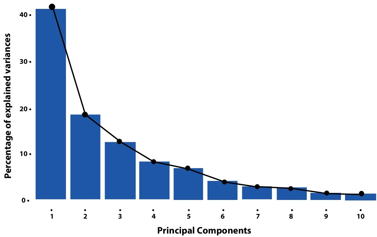
Figure 8.3 Five variances acquired by PCs.
These limitations can be overcome by bringing slight changes to the method. Some generalised forms of PCA have been created which vanquish its disadvantages, such as Sparse PCA, KPCA or Non-Linear PCA, Probabilistic PCA, Robust PCA, to name a few. Sparse PCA overcomes the disadvantage of PCs being a combination of all the input variables by adding a sparsity constraint on the input variables. Thus, making PCs a combination of only a few input variables. The Non-Linear PCA works on the nature of this traditional method and uses a kernel trick to make it suitable for non-linear datasets as well. Probabilistic PCA makes the method more efficient by making use of Gaussian noise model and a Gaussian prior. Robust PCA works well with corrupted datasets.
8.3.2 Linear Discriminant Analysis
Linear Discriminant Analysis (LDA), also known as discriminant function analysis, is one of the most commonly used linear dimensionality reduction techniques. It performs supervised dimensionality reduction by projecting input data to a linear subspace consisting of directions that maximise the separation between classes. In short, it produces a combination of variables or features in a linear manner, for characteristics of classes. Although, it should be duly noted that to perform LDA, continuous independent variables must be present, as it does not work on categorical independent variables.
LDA is similar to PCA but is supervised, PCA doesn’t take labels into consideration and thus, is unsupervised. Also, PCA focuses on feature classification, on the other hand, LDA carries out data classification. LDA also overcomes several disadvantages of Logistics Regression, another algorithm for linear classification which is works well for binary classification problems. LDA can handle multi-class classification problems with ease.
LDA concentrates on maximising the distance among known categories and it does by creating a new axis in the case of Two-Class LDA and multiple axes in the case of Multi-Class LDA in a way to maximise the separation between known categories. The new axis/axes are created according to the following criteria which are considered simultaneously.
8.3.2.1 Two-Class LDA
- Maximise the distance between means of both categories.
- Minimise the variation (which LDA calls “scatter”) within each category (refer Figure 8.4).
8.3.2.2 Three-Class LDA
In the case of Multi-Class LDA, the number of categories/classes are more than two and there is a slight difference from the process used in Two-Class LDA:
- We first find the point that is central to all of the data.
- Then measure the distances between a point that is central in each category and the main central point.
- Now maximise the distance between each category and central point while minimising the scatter in each category (refer Figure 8.5).
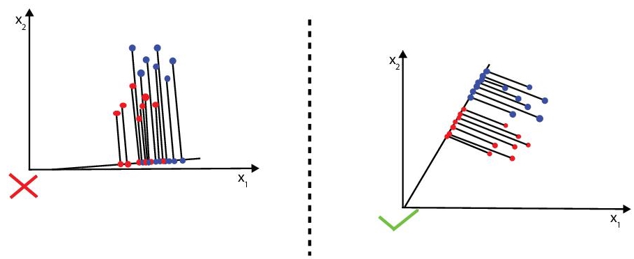
Figure 8.4 Two class LDA.

Figure 8.5 Choosing the best centroid for maximum separation among various categories.
While the ideas involved behind LDA are quite direct, but the mathematics involved is complex than those on which PCA is based upon. The goal is to find a transformation such that it will maximise the between-class distance and minimise the within-class distance. [Reference] For this we define two matrices: within-class scatter matrix and between-class scatter matrix.
The steps involved while performing LDA are:
- Given the samples X1, X2,……., Xn, and their respective labels y1, y2,……, yn, the within-class matrix is computed as:
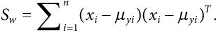 (8.7)
(8.7)where,
 , (mean of
  class) and Ni = number of data samples in class Xi.
 - The between-class matrix is computed as:
 (8.8)
(8.8)where
 (i.e. overall mean of whole sample), and
  (i.e. mean of kth class).
 - We are looking for a projection that maximises the ratio of between-class to within-class scatter and LDA is actually a process to do so. We use the determinant of scatter matrices to obtain a scalar function:
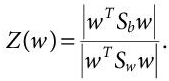 (8.9)
(8.9) - Then, we differentiate the above term with respect to w, to maximise Z(w). Hence, the eigen value problem can be generalised to K-classes as:
 (8.10)
where, λi = J(wi) = scalar and i = 1, 2… (K-1).
- Finally, we sort the eigenvectors in a descending order and choose the top Eigenvectors to make our transformation matrix used to project our data.
This analysis is carried out by making a number of assumptions, which generates admirable results and leads to outperforming other linear methods. In [10], Paul Murray et al. showed how LDA was superior to PCA for performing experiments for inspection of rice-seed quality. These assumptions include multivariate normality, homogeneity of variance/covariance, multicollinearity and independence of participants’ scores of features. LDA generates more accurate results when the sample sizes are equal.
The high applicability of LDA is a result of the advantages offered by it. Not only its ability to handle large and multi-class datasets is high, but also, it is less sensitive to faults. Also, it is very reliable when used on dichotomous features. It supports both binary and multi-class classifications. Apart from being the first algorithm used for bankruptcy prediction of firms, it has served as a pre-processing step in many applications such as statistics, bio-medical studies, marketing, pattern recognition, image recognition, and other machine learning applications. As any other technique, LDA also suffers from some drawbacks. While using LDA, lack of sample data leads to degraded classifier performance. A large number of assumptions in LDA also make it difficult for usage. Sometimes, it fails to preserve the complex structure of data, and is not suitable for non-linear mapping of data-points. LDA collapses when mean of the distributions are shared. This disadvantage came be eliminated by the use of Non-linear discriminant analysis.
Linear Discriminant Analysis has many extended forms, such as Quadratic Discriminant Analysis (QDA), Flexible Discriminant Analysis (FDA) and Regularised Discriminant Analysis (RDA). In Quadratic Discriminant Analysis, each class uses its own covariance/variance. In FDA, combinations of input are used in a non-linear Manner. RDA focusses on regularising the estimation of covariance.
8.3.3 Kernel Principal Component Analysis
Kernel Principal Component Analysis (KPCA) or Non-Linear PCA is one of the extended forms of PCA [11, 12]. The main idea behind this method is to modify the non-linear dataset in such a way that it becomes linearly separable. This is done by mapping the original dataset to a high-dimensional feature space, x→ ϕ(x) (ϕ is the non-linear mapping function of the sample x), and this results in a linearly separable dataset and now PCA can be applied on it for dimensionality reduction. But, carrying out calculations in the feature space can be very expensive, and basically infeasible, due to the high dimensionality of the feature space. So, we use kernel methods to carry out the mapping. It can be represented as follows:

Figure 8.6 Kernel principal component analysis.
The kernel methods perform implicit mapping using a kernel function, which basically calculates the dot product of the feature vectors to perform non-linear mapping [11, 13] (refer Figure 8.6).
Here, K is the kernel function. This is the central equation in the kernel methods. Now, the choice of kernel functions play a very significant roles the result of the entire method depends on it. Some of them are Linear kernel, Polynomial kernel, Sigmoid kernel, Radial Basis Function (RBF) kernel, Gaussian kernel, Spline kernel, Laplacian Kernel, Hyperbolic Tangent Kernel, Bessel kernel, etc. If the kernel function is linear, KPCA works similar to PCA and performs a linear transformation. When using polynomial kernel, the central equation can be stated as:
Here, d is the degree of polynomial and we assume that the data points have zero mean. In Sigmoid kernel, which is popular in neural networks, the equation gets transformed to (with the assumption that the data points have zero mean):
The Gaussian kernel is used when there is no prior knowledge of the data. The equation used is:
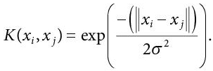 (8.14)
Here, again the data points are assumed to have zero mean. In case, the data points don’t have zero mean, a normalisation content is added to the gaussian kernel’s equation,  Adding this constant makes the Gaussian kernel a normalised kernel, and the modified equation can be written as:
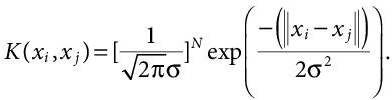 (8.15)
The Radial Basis Function (RBF) kernel is the most used due to its localised and finite response along the entire x-axis. It has many different types including Gaussian radial basis function kernel, Laplace radial basis function kernel, etc. the basic equation for the RBF kernel is:
The procedure followed for execution of the KPCA method is:
- The initial step is to select a type of kernel function K(xi, xj). ϕ is the transformation to higher dimension.
- The Covariance matrix is generated after selecting the kernel function. In KPCA, the covariance matrix is called the Kernel matrix. It is generated by performing inner product of the mapped variables. It can one written as:
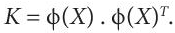 (8.17)
This is called the kernel trick. It helps to avoid the necessity of explicit knowledge of φ.
- The kernel matrix generated in the previous step is then normalised by using:
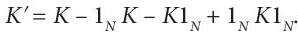 (8.18)
Here, 1N is a N*N matrix with all entries equal to (1/N). This step makes sure that the mapped features, using the kernel function, are zero-mean. Chis cantering operation performs subtraction of the mean of the data in feature space, defined by the kernel function.
- Now, the eigenvectors and eigenvalues of the centred kernel matrix are calculated. The eigenvector equation is used to calculate and normalise the eigenvectors:
 (8.19)
Here, αi denotes the eigenvectors.
- The step is similar to the third step of the PCA. here, eigenvectors generate the Principal Components in the feature space, and further they are ranked in decreasing order on the basis of their eigenvalues. The Principal Component with the highest eigenvalue possesses maximum variance. Adequate components are then selected to map the data points on them in such a manner that the variance is maximised. The selected components are represented using a matrix.
- The last step is to find the low dimensional representation which is done my mapping the data onto the selected components in the previous step. It can be done by finding the product of the initial dataset and the matrix obtained in the 5th step.
The results of de-noising images using linear PCA and KPCA have been shown in Figure 8.7. It can be observed that KPCA outperforms PCA in this case.
The kernel trick has been used in many techniques of the Machine Learning domain, such as Support vector machines, kernel ridge regression, etc. It has been proved useful for many applications, such as: Novelty detection, Speech recognition, Face recognition, Image de-noising, etc. The major advantage it offers is that it allows modification of linear methods to enable them to work on non-linear datasets and generate highly accurate results. Being a generalised version of PCA, KPCA owns all the advantages offered by PCA. Even though it overcomes the largest disadvantage of linear nature of PCA, it still has some limitations. To start with, the size of kernel mart is proportional to the square of variables of original dataset. On the top of this, KPCA focuses on retaining large pairwise distances. The training time required by this method is also very high. And due to its non-linear nature, it becomes more sensitive to fault when compared to PCA. Minh Hoai Nguyen et al. [17] proposed a robust extension of KPCA, called Robust KPCA, which showed better results for de-noising images, recovering missing data and handling intra-sample outliers. It outperformed other methods of same nature when experiments were conducted on various natural datasets. Many such methods have been proposed which mitigates the disadvantages offered by KPCA. Sparse KPCA is one of them. A. Lima et al. [13] proposed a version of Sparse KPCA for Feature Extraction in Speech Recognition. It treats the disadvantage of training data reduction in KPCA when the dataset is excessively large. This approach provided better results than PCA and KPCA on a Japanese ATR database (refer Figure 8.8).
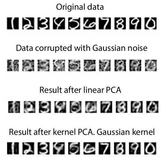
Figure 8.7 Results of de-noising handwritten digits.

Figure 8.8 Casting the structure of Swiss Roll into lower dimensions.
8.3.4 Locally Linear Embedding
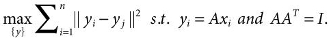
Locally Linear Embedding (LLE) is a non-linear technique for dimensionality reduction that preserves the local properties of data, it could mean preserving distances, angles or it could be something entirely different. It aims at maintaining the global construction of datasets by locally linear reconstructions. Being an unsupervised technique, class labels don’t hold any importance for this analysis. Datasets are often represented in n-Dimensional feature space, with each dimension used for a specific feature. Many other algorithms of dimensionality reduction fail to be successful on non-linear space. LLE reduces these n-dimensions by preserving the geometry of the structure locally while piecing local properties together to preserve the structure globally. The resultant structure is casted into lower dimensions. In short, it makes use of local symmetries of the linear reconstructions to work with non-linear manifolds.
Simple geometric intuitions are the principle behind the working of LLE [Reference]. The procedure for Locally Linear Embedding algorithm includes three basic steps, which are as follows:
- LLE first computes the K nearest neighbours in which a point or a data vector is classified on basis of its nearest K neighbours but we have to careful while selecting the value of K, as K is the only parameter chosen and if too small or too big value is chosen, it will fail to preserve the geometry globally.
-
Then, a set of weights [Wij] are computed, for each neighbour which denotes the effect of neighbour on that data vector. The weights cannot be zero and the cost function should be minimised as shown below:
 (8.20)
Where jth is the index for nearest neighbour of point Xi.
- Finally, we construct the low dimensional embedding of vector Y with the previously computed weights, and we do it by minimising the cost function below:
 (8.21)
In the achieved low- dimensional embedding, each point can still be represented with the same linear integration of its neighbours, as the one in the high dimensional representation.
LLE is an efficient algorithm particularly in pattern recognition tasks where the distance between the data points is an important factor in the algorithm and want to save computational time. LLE is widely used in pattern recognition, super-resolution, sound-source localisation, image processing problems and it shows significant results. It offers a number of advantages over other existing non-linear methods, such as: Non-linear PCA, Isomap, etc. Its ability to handle non-linear manifolds is commendable as it holds the capacity to identify a curved pattern in the structures of datasets. It even offers lesser computational time and memory as compared to other techniques. Also, it involves tuning only one parameter ‘K’ i.e., the number of nearest neighbours, therefore making the algorithm less complex. Although, some drawbacks of LLE exist, such as its poor performance when it encounters a manifold with holes. It also slumps large portions on data very close together when in the low dimensional representation. Such drawbacks have been removed by bringing slight modifications to the original analysis or generating extended versions of the algorithm. Hessian LLE (HLLE) is an example of an extension of LLE, which reduces the curviness of the original manifold while mapping it onto a low-dimensional subspace. Refer Figure 8.9 for Low dimensional Locally linear Embedding.
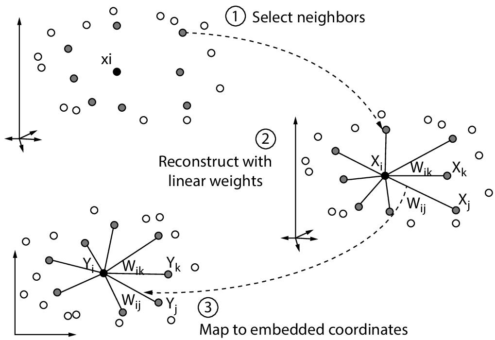
Figure 8.9 Working of LLE.
8.3.5 Independent Component Analysis
As we learned about PCA that it is about finding correlations by maximizing variances whereas in ICA we try to maximize independence by finding a linear transformation for our feature space into a new feature space such that each of the individual new features are mutually independent statistically. ICA does an excellent job in Blind Source Separation (BSS) wherein it receives a mixture of signals with very little information about the source signals and it separates the signals by finding a linear transformation on the mixture such that the output signals are statistically independent i.e. if sources{si} are statistically independent then:
Here, {si} follows the non-gaussian distribution.
PCA does a poor job in Blind Source Separation. A common application of BSS is the cocktail party problem. The set of individual source signals are represented by s(t) = {s1(t), s2(t), ....sn(t)}. Source signals (s(t)) are mixed with a mixing matrix (A) which produce the mixed signals (x(t)). So, mathematically we could express the relation as follows: where, there are two signal sources (s1 & s2) and A (mixing matrix) contains the coefficients (a, b, c, d) of linear transformation.
 (8.23)
The relation above is under some following assumptions:
- The mixing matrix (A) is invertible.
- The independent components have non-gaussian distributions.
- The sources are statistically independent.
To solve the above problem and recover our original strings from the mixed ones, we need to solve equation (1) for s(t) given by relation:
Here, A-1 is called un-mixing matrix (W) and we need to find this inverse matrix to find our original sources and choose the numbers in this matrix in such a way that maximizes the probability of our data.
Independent Component Analysis is used in multiple fields and applications such as telecommunications, stock prediction, seismic monitoring, text document analysis, optical imaging of neurons and often applied to reduce noise in natural images.
8.3.6 Isometric Mapping (Isomap)
Isomap (IM), short for Isometric mapping, is a non-linear extended version of Multidimensional Scaling (MDS). It focuses on preserving the overall geometry of the input dataset, by making use of a weighted neighbourhood graph ‘G’ for performing low dimensional embedding of the initial data in high-dimensional manifold. Unlike MDS, it aims at sustaining the Geodesic pairwise distance between all the data points. The concept and procedure followed by Isomap is very similar to Locally Linear Embedding (LLE), except the fact that the latter focuses on maintaining the local structure of the data while carrying out transformation, whereas Isomap is more inclined towards conserving the global structure along with the local geometry of the data points.
The IM algorithm executes the following three steps to procure a low dimensional embedding:
- The procedure starts with the formation of a neighbourhood weighted graph G, by considering ‘k’ nearest neighbours of the data points xi (i=1, 2,…,n), where the edge weights are equal to the Euclidean distances. This steps ensures that local structure of the dataset does not get compromised.
- The next step is to determine the geodesic distances, and form a Geodesic distance matrix. Geodesic distance can be defined as the sum of edge weights and the shortest path between two data points. This is done by making use of Dijkstra’s algorithm or Floyd-Warshall shortest path algorithm. It is the distinguishing step between Isomap and MDS.
- The last step is to apply MDS on the matrix obtained in the previous step.
Preserving the curvilinear distances over a manifold is the biggest advantage offered by Isomap as usage of Euclidean distances over a curved manifold can generate misleading results. Geodesic distance helps to overcome this issue faced by MDS. Isomap has been successfully applied to various applications such as: Pattern Recognition, Wood inspection, Image processing, etc. A major flaw Isomap suffers with is short circuiting errors, which occur due to inaccurate connectivity in the graph G. A. Saxena et al. [28] overcame this issue by removing certain neighbours that caused issues in determining the local linearity of the graph. It has also failed under circumstances where the manifold was non-convex and if it contains holes.
Many Isomap generalisations have been created over the years, which include: Conformal Isomap, Landmark Isomap and Parallel transport unfolding. Conformal Isomap or C-Isomap owns the ability to understand curved manifold in a better way, by magnifying highly dense sections of the manifold, and narrowing down the regions with less intensity of data points. Landmark Isomap (L-Isomap) reduces the computational complexity by considering a marginal amount of landmark points out of the entire set. Parallel transport unfolding works on removing the voids and irregularity in sampling by substituting the geodesic distances for parallel transport-based approximations. In [8], Vin de Silva et al. presented an improved approach to Isomap and derived C-Isomap and L-Isomap algorithms which exploited computational sparsity.
8.3.7 Self-Organising Maps
Self-Organising Map (SOM) are unsupervised neural networks that are used to project high-dimensional data into low-dimensional output which is easy to visualize and understand. Ideas were first introduced by C. von der Malsburg in 1973 but developed and refined by T. Kohonen in 1982. SOMs are mainly used for clustering (or classification), data visualization, probability, modelling and density estimation. There are no hidden layers in these neural networks and only contains an input and output layer. SOM uses Euclidean distances to plot data points and the neutrons are arranged on 2-dimensional grid also called as a map.
First, we initialize neural network weights randomly and choose a random input vector from training dataset and also set a learning rate (η).
Then for each neuron j, compute the Euclidean distance:
Here, xi is the current input vector and wij is the current weight vector.
We then select the winning neutron (Best Matching Unit) with index j such that D(j) is minimum and then we update the network weights given by the equation:
Here, (t) (learning rate) = ƞ0exp (− t /λ), t = epoch, λ = time constant. The learning rate decay is calculated for every epoch.
 (8.27)
Where, σ is called the Neighbourhood Size which keeps on decreasing as the training continues given by an exponential decay function:
 (8.28)
The influence rate signifies the effect of a node distance from the selected neutron (BMU) has its own learning and finally through many iterations and updating of weights, SOM reaches a stable configuration.
Self-organising maps are applied to wide range of fields and applications such as in analysis of financial stability, failure mode and effect analysis, classifying world poverty, seismic facies analysis for oil and gas exploration etc. and is a very powerful tool to visualize the multi-dimensional data.
8.3.8 Singular Value Decomposition
SVD is a linear dimensionality reduction technique which basically gives us the best axis to project our data in which the sum of squares of projection error is minimum. In other words, we can say that it allows us to rotate the axes in which the data is plotted to a new axis into a new axis along the directions that have maximum variance. It is based on simple linear algebra which makes it very convenient to use it on any data matrix where we have to discover latent, hidden features and any other useful insights that could help us in classification or clustering. In SVD an input data matrix is decomposed into three unique matrices:
where A: [m x n] input data matrix, U: [m x m] real or complex unitary matrix (also called left singular vectors), ∑: [m x n] diagonal matrix, and V: [n x n] real or complex unitary matrix (also called right singular vectors).
U and V are column orthonormal matrices, meaning the length of each column vector is one. The values in ∑ matrix is called singular values and they are positive and sorted in decreasing order, meaning the largest singular values come first.
SVD is widely used in many different applications like in recommender systems, signal processing, data analysis, latent semantic indexing and pattern recognition etc. and is also used in performing Principal Component Analysis (PCA) in order to find principal directions which, have the maximum variance. Also, the rotation in SVD helps in removing collinearity in the original feature space. SVD doesn’t always work well specially in cases of strongly non-linear data and its results are not ideal for good visualizations and while it is easy to implement the algorithm but at the same time it is computationally expensive.
8.3.9 Factor Analysis
Factor Analysis is a variable reduction technique which primarily aims at removing highly redundant data in our dataset. It does so by removing highly correlated variable into small numbers of latent factors. Latent factors are the factors which are not observed by us but can be deduced from other factors or variables which are directly observed by us. There are two types of Factor Analysis: Exploratory Factor Analysis and Confirmatory Factor Analysis. The former focuses on exploring the pattern among the variables with no prior knowledge to start with while the later one is used for confirming the model specification.
Consider the following matrix equation from which Factor analysis assumes its observable data that has been deduced from latent factors:
Here, x is a set of observable random variables with means µ. L contains the unknown constants and F contains “Common Factors” which are unobserved random variables and influences the observed variables. ε is the unobserved error terms or the noise which is stochastic and have a finite variance.
The common factors matrix(F) is under some assumptions:
- F and ε are independent.
- Corr(F) = I (Identity Matrix), here, “Corr” is the cross-covariance matrix.
- E(F) = 0 (E is the Expectation).
Under these assumptions, the covariance matrix of observed variables [Reference] is:
Taking Corr(y) = ∑ and Corr(ε) = λ, we get ∑ = LLT + λ. The matrix L is solved by the factorization of matrix LLT = ∑ - λ.
We should consider that prior to performing Factor Analysis the variables are following multivariate normal distribution and there must be large number of observations and enough number of variables that are related to each other in order to perform data exploration to simplify the given dataset but if observed variables are not related, factor analysis will not be able to find a meaningful pattern among the data and will not be useful in that case. Also, the factors are sometimes hard to interpret so it depends on researcher’s ability to understand it attributes correctly.
8.3.10 Auto-Encoders
Auto-Encoders are unsupervised practical implementation of otherwise supervised neural networks. Neural networks are basically a string of algorithms, that try to implement the way in which human brain processes the gigantic amount of data. In short, neural networks tend to identify the underlying pattern behind how the data is related, and thus perform classification and clustering in a way similar to a human brain. Auto-encoder performs dimensionality reduction by achieving reduced representation of the dataset with the help of a bottleneck, also called the hidden layer(s). The first half portion of an auto-encoder encodes the data to obtain a compressed representation, while the second half focuses on regenerating the data from the encoded representatives. The simplest form of an auto-encoder consists of three layers: The Input layer, the hidden layer (bottleneck) and the output layer.
The architecture of an auto-encoder can be well explained in two steps:
- Encoder: This part of an auto-encoder accepts the input data, using the input layer. Let x ∈ Rd be the input. The hidden layer (bottleneck) maps this data onto H, such that H ∈ RD. where H is the low dimensional representation of the input X. Also,
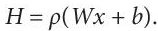 (8.32)
Where ⍴ is the activation function, W denotes the Weight matrix and b is the bias vector.
- Decoder: This part is used for reconstruction of the data from the reduced formation achieved in the previous step. The output generated by it is expected to be the same as the input. Let x′ be the reconstruction, which is of the same shape as x, then x′ can be represented as:
 (8.33)
Here, ⍴′, W′ and b′ might not be same as in equation (8.32).
The entire auto-encoder working can be expressed in the following equations:
Where F is the feature space and H ∈ F, ϕ and ψ are the transitions in the two phases and X and X’ are the input and output spaces, which are expected to coincide perfectly.
The existence of more than 1 hidden-layers give birth to Multilayer auto-encoders. The concept of Auto-encoders has been successfully applied various applications which include information retrieval, image processing, Anomaly detection, HIV analysis etc. It makes use of the phenomenon of back-propagation to minimise the reconstruction loss, and also for training of the auto-encoder. Although back propagation converges with increasing number of connections, which serves as a drawback. It is overcome by pre-training of the auto-encoder, using RBMs. In [9], Omprakash Saini et al. stated poor interpretability as one of its other drawbacks, and pointed out various other advantages, such as, its ability to adopt parallelization techniques for improving the computations.
8.4 Experimental Analysis
8.4.1 Datasets Used
In following experiments, we reduce the feature set of two different datasets using both linear and non-linear dimension reduction techniques. We would also compute accuracy of predictions of each technique and lastly compare the performance of techniques used in this experimental analysis.
Datasets used are as following:
- Red-Wine Quality Dataset: The source of this dataset is UCI which is a Machine Learning repository. The wine quality dataset has two datasets, related to red and white wine samples of Portugal wines. For this paper, Red wine dataset issued which consists of 1599 instances and 12 attributes. It can be viewed as classification and regression tasks.
- Wisconsin Breast Cancer Dataset: This dataset was also taken from UCI, a Machine Learning repository. It is a multivariate dataset, containing 569 instances, 32 attributes and no missing values. The features of the dataset have been computed by using digitised images of FNA of a breast mass.
8.4.2 Techniques Used
- Linear Dimensionality Reduction Techniques: Principal Component Analysis (PCA), Linear Discriminant Analysis (LDA), Independent Component Analysis (ICA), Singular Value Decomposition (SVD).
- Non-Linear Dimensionality Reduction Techniques: Kernel Principal Component Analysis (KPCA), Locally Linear Embedding (LLE).
8.4.3 Classifiers Used
- In case of Red Wine Quality Dataset, Random Forest algorithm is used to predict the quality of red wine.
- For prediction in Wisconsin Breast Cancer Dataset, Support-Vectors Machine (SVM) classifier is used.
8.4.4 Observations
Dimensionality Reduction Techniques Results on RED-WINE Quality Dataset (1599 rows X 12 columns), using Random Forest as classifier, have been shown in Table 8.2.
Table 8.3 shows the Dimensionality Reduction Techniques Results on WISCONSIN BREAST-CANCER Quality Dataset (569 rows X 33 columns) using SVM as classifier.
8.4.5 Results Analysis Red-Wine Quality Dataset
- Both PCA and LDA shows the highest accuracy of 64.6% correct predictions among all the techniques used.
- Both the techniques reduce the dimensions of dataset from 12 to 3 most important features.
- Non-Linear techniques used i.e. KPCA & LLE doesn’t perform well on this dataset and all the Linear Dimensionality Reductions techniques outperformed the non-linear techniques.
Wisconsin Breast Cancer quality dataset
- PCA technique shows the best accuracy among all the techniques with an error rate of only 2.93%, which means over 97% of the cases were predicted correctly.
- PCA reduces the dimension of dataset from 33 features to 5 most important features to achieve its accuracy.
- Again, the Linear Reduction techniques outperformed the non-linear techniques used in this dataset.
Table 8.2 Results of red-wine quality dataset.
| Dimension reduction techniques | Total number of data rows | Number of actual dimensions | Number of reduced dimensions | Correct prediction % | Error % |
|---|---|---|---|---|---|
| PCA | 1599 | 12 | 3 | 64.6% | 35.4% |
| LDA | 1599 | 12 | 3 | 64.6% | 35.4% |
| KPCA | 1599 | 12 | 1 | 44.06% | 55.94% |
| LLE | 1599 | 12 | 1 | 42.18% | 57.82% |
| ICA | 1599 | 12 | 3 | 65.31% | 34.69% |
| SVD | 1599 | 12 | 3 | 64.48% | 35.52% |
Table 8.3 Results of Wisconsin breast cancer quality dataset.
| Dimension reduction techniques | Total number of data rows | Number of actual dimensions | Number of reduced dimensions | Correct prediction % | Error % |
|---|---|---|---|---|---|
| PCA | 569 | 33 | 5 | 97.07% | 2.93% |
| LDA | 569 | 33 | 3 | 95.9% | 4.1% |
| KPCA | 569 | 33 | 1 | 87.71% | 12.29% |
| LLE | 569 | 33 | 1 | 87.13% | 12.87% |
| ICA | 569 | 33 | 3 | 70.76% | 29.24% |
| SVD | 569 | 33 | 4 | 95.9% | 4.1% |
8.5 Conclusion
Although, researchers have been working on finding techniques to cope up with the high dimensionality of data, which serves as a disadvantage, for more than a hundred years now, the challenging nature of this task has evolved with all the progress in this field. Researchers have come a long way since 1900s, when the concept of PCA first came into existence. However, from the experiments performed for this research work, it can be concluded that the linear and the traditional techniques of Dimensionality Reduction still outperform the non-linear ones. This conclusion is apt for most of the datasets. The results generated by PCA make it the most desirable tool. The error percentage of the contemporary, non-linear techniques make them inapposite. Having said that, research work is still in its initial stages for the huge, non-linear datasets and proper exploration and implementation of these techniques can lead to generation of fruitful results. In short, the benefits being offered by the non-linear techniques can be fully enjoyed by doing more research and improving the pitfalls.
References
- 1. Mishra, P.R. and Sajja, D.P., Experimental survey of various dimensionality reduction techniques. Int. J. Pure Appl. Math., 119, 12, 12569–12574, 2018.
- 2. Sarveniazi, A., An actual survey of dimensionality reduction. Am. J. Comput. Math., 4, 55–72, 2014.
- 3. Bartenhagen, C., Klein, H.-U., Ruckert, C., Jiang, X., Dugas, M., Comparative study of unsupervised dimension reduction techniques for the visualization of microarray gene expression data. BMC Bioinf., 11, 1, 567–577, 2010.
- 4. Patil, M.D. and Sane, S.S., Dimension reduction: A review. Int. J. Comput. Appl., 92, 16, 23–29, 2014.
- 5. Globerson, A. and Tishby, N., Most informative dimension reduction. AAAI-02: AAAI-02 Proceedings, pp. 1024–1029. Edmonton, Alberta, Israel, August 1, 2002.
- 6. Nelson, D. and Noorbaloochi, S., Sufficient dimension reduction summaries. J. Multivar. Anal., 115, 347–358, 2013.
- 7. Ma, Y. and Zhu, L., A review on dimension reduction. Int. Stat. Rev., 81, 1, 134–150, 2013.
- 8. de Silva, V. and Tenenbaum, J.B., Global versus local methods in nonlinear dimensionality reduction. NIPS’02: Proceedings of the 15th International Conference on Neural Information Processing, pp. 721–728, MIT Press, MA, United States, 2002.
- 9. Saini, O. and Sharma, P.S., A review on dimension reduction techniques in data mining. IISTE, 9, 1, 7–14, 2018.
- 10. Fabiyi, S.D., Vu, H., Tachtatzis, C., Murray, P., Harle, D., Dao, T.-K., Andonovic, I., Ren, J., Marshall, S., Comparative study of PCA and LDA for rice seeds quality inspection. IEEE Africon, pp. 1–4, Accra, Ghana, IEEE, September 25, 2019.
- 11. Tippin, M.E., Sparse kernel principal component analysis. NIPS’00: Proceedings of the 13th International Conference on Neural Information Processing Systems, United States, MA, January 2000, MIT Press, pp. 612– 618,, MIT Press, United States, MA, January 2000.
- 12. Kim, K., II, Jung, K., Kim, H.J., Face recognition using kernel principal component analysis. IEEE Signal Process. Lett., 9, 2, 40–42, 2002.
- 13. Lima, A., Zen, H., Nankaku, Y., Tokuda, K., Kitamura, T., Resende, F.G., Sparse KPCA for feature extraction in speech recognition. IEICE Trans. Inf. Syst., 1, 3, 353–356, 2005.
- 14. Yeung, K.Y. and Ruzzo, W.L., Principal component analysis for clustering gene expression data. OUP, 17, 9, 763–774, 2001.
- 15. Raychaudhuri, S., Stuart, J.M., Altman, R.B., Principal component analysis to summarize microarray experiments: Application to sporulation time series. Pacific Symposium on Biocomputing, vol. 5, pp. 452–463, 2000.
- 16. Hinton, G.E. and Salakhutdinov, R.R., Reducing the dimensionality of data with neural networks. Sci. AAAS, 313, 5786, 504–507, 2006.
- 17. Nguyen, M.H. and De la Torre, F., Robust kernel principal component analysis, in: Advances in Neural Information Processing Systems 21: Proceedings of the Twenty-Second Annual Conference on Neural Information Processing Systems; Vancouver, British Columbia, Canada, December 8-11, 2008. 185-119, Curran Associates, Inc., NY, USA, 2008.
- 18. Raymer, M.L., Punch, W.F., Goodman, E.D., Kuhn, L.A., Jain, A.K., Dimensionality reduction using genetic algorithms. IEEE Trans. Evol. Comput., 4, 2, 164–171, 2000.
- 19. DeMers, D. and Cottre, G., Non-linear dimensionality reduction. Advances in Neural Information Processing Systems, 5, 1993; 580-587, NIPS, Denver, Colorado, USA, 1992.
- 20. Tenenbaum, J.B., de Silva, V., Langford, J.C., A global geometric framework for nonlinear dimensionality reduction. Sci. AAAS, 290, 5500, 2319–2323, 2000.
- 21. Zhang, D., Zhou, Z.-H., Chen, S., Semi-supervised dimensionality reduction. Proceedings of the Seventh SIAM International Conference on Data Mining, Minneapolis, Minnesota, USA, April 26-28, Society for Industrial and Applied Mathematics, 3600 University City Science Center, Philadelphia, PA, United States, pp. 11–393, 2007.
- 22. Sarwar, B.M., Karypis, G., Konstan, J.A., Riedl, J.T., Application of dimensionality reduction in recommender system–a case study. ACM WEBKDD Workshop: Proceedings of ACM WEBKDD Workshop, USA, 2000, p. 12, Association for Computing Machinery, NY, USA, 2000.
- 23. Raich, R., Costa, J.A., Damelin, S.B., Hero III, A.O., Classification constrained dimensionality reduction. ICASSP: Proceedings ICASSP 2005, Philadelphia, PA, USA, March 23, 2005, IEEE, NY, USA, 2005.
- 24. van der Maaten, L.J.P., Postma, E.O., van den Herik, H.J., Dimensionality reduction: A comparative review. J. Mach. Learn. Res., 10, 1, 24, 66–71, 2007.
- 25. Adragni, K.P. and Cook, R.D., Sufficient dimension reduction and prediction in regression. Phil. Trans. R. Soc. A, 397, 4385–4405, 2009.
- 26. Alam, M.A. and Fukumizu, K., Hyperparameter selection in kernel principal component analysis. J. Comput. Sci., 10, 7, 1139–1150, 2014.
- 27. Wang, Q., Kernel principal component analysis and its applications in face recognition and active shape models. Corr, 1207, 3538, 27, 1–8, 2012.
- 28. Hamdi, N., Auhmani, K., M’rabet Hassani, M., Validation study of dimensionality reduction impact on breast cancer classification. Int. J. Comput. Sci. Inf. Technol., 7, 5, 75–84, 2015.
- 29. Vlachos, M., Dimensionality reduction KDD ‘02: Proceedings of the eighth ACM SIGKDD International Conference on Knowledge Discovery and Data Mining Edmonton, Alberta, Alberta 2002, pp. 645–651, Association for Computing Machinery, NY, United States, 2002.
- 30. Sembiring, R.W., Zain, J.M., Embong, A., Dimension reduction of health data clustering. Int. J. New Comput. Archit. Appl., 1, 3, 1041–1050, 2011.
- 31. Wang, W. and Carreira-Perpinan, M.A., The role of dimensionality reduction in classification. AAAI Conference on Artificial Intelligence, Québec City, Québec, Canada, July 27–31, 2014, AAAI Press, Palo Alto, California, pp. 1–15, 2014.
- 32. Cunningham, P., Dimension reduction, in: Technical Report UCD-CSI, pp. 1–24, 2007.
- 33. Partridge, M. and Sedal, R.C., Fast dimensionality reduction and simple PCA. Intell. Data Anal., 2, 3, 203–214, 1998.
- 34. Voruganti, S., Ramyakrishna, K., Bodla, S., Umakanth, E., Comparative analysis of dimensionality reduction techniques for machine learning. Int. J. Sci. Res. Sci. Technol., 4, 8, 364–369, 2018.
- 35. Varghese, N., Verghese, V., Gayathri, P., Jaisankar, D.N., A survey of dimensionality reduction and classification methods. IJCSES, 3, 3, 45–54, 2012.
- 36. Fodor, I.K., A Survey of Dimension Reduction Techniques, pp. 1–18, Center for Applied Scientific Computing, Lawrence Livermore National Laboratory, 2002.
- 37. Roweis, S.T. and Saul, L.K., Nonlinear dimensionality reduction by locally linear embedding. Sci. AAAS, 290, 5500, 2323–2326, 2000.
- 38. Govinda, K. and Thomas, K., Survey on feature selection and dimensionality reduction techniques. Int. Res. J. Eng. Technol., 3, 7, 14–18, 2016.
- 39. Sembiring, R.W., Zain, J.M., Embong, A., Alternative model for extracting multidimensional data based-on comparative dimension reduction, in: CCIS: Proceedings of International Conference on Software Engineering and Computer Systems, Pahang, Malaysia, June 27-29, 2011 Springer, Berlin, Heidelberg, Malaysia, pp. 28–42, 2011.
- 40. Ji, S. and Ye, J., Linear dimensionality reduction for multi-label classification, in: Twenty-First International Joint Conference on Artificial Intelligence, Pasadena, California, June 26, 2009, AAAI Press, pp. 1077–1082, 2009.
- 41. Wang, Y. and Lig, Z., Research and implementation of SVD in machine learning. IEEE/ACIS 16th International Conference on Computer and Information Science (ICIS), Wuhan, China, May 24-26, 2017, IEEE, NY, USA, pp. 471– 475, 2017.
- 42. Kaur, S. and Ghosh, S.M., A survey on dimension reduction techniques for classification of multidimensional data. Int. J. Sci. Technol. Eng., 2, 12, 31–37, 2016.
- 43. Chipman, H.A. and Gu, H., Interpretable dimension reduction. J. Appl. Stat., 32, 9, 969–987, 2005.
- 44. Ali, A. and Amin, M.Z., A Deep Level Understanding of Linear Discriminant Analysis (LDA) with Practical Implementation in Scikit Learn, pp. 1–12, Wavy AI Research Foundation, 2019. https://www.academia.edu/41161916/A_Deep_Level_Understanding_of_Linear_Discriminant_Analysis_LDA_with_Practical_Implementation_in_Scikit_Learn
- 45. Hyvarinen, A., Survey on independent component analysis. Neural Comput. Surv., 2, 4, 94–128, 1999.
- 46. Nsang, A., Bello, A.M., Shamsudeen, H., Image reduction using assorted dimensionality reduction techniques. Proceedings of the 26th Modern AI and Cognitive Science Conference, Greensboro, North Carolina, USA, April 25–26, 2015, MAICS, Cincinnati, OH, pp. 121–128, 2015.
Note
- *Corresponding author: [email protected]