
Chapter 3
Recognizing Images with CNNs
IN THIS CHAPTER
![]() Performing basic image recognition
Performing basic image recognition
![]() Working with convolutions
Working with convolutions
![]() Looking for edges and shapes in images
Looking for edges and shapes in images
Humans are graphically (visually) oriented, but computers aren’t. So, the task that humans most want performed by deep learning — recognizing items in images — is also one of the harder tasks to perform using a computer. The manner in which a computer deals with images is completely different from humans. When working with images, computers deal with the numeric values that make up individual pixels. The computer processes the numbers used to create an image much as it processes any other group of numbers. Consequently, this chapter deals with using a different kind of math to manipulate those pixel values so that a computer can output the desired result, despite having no concept whatsoever that it is even processing an image.
You have some methods of working with images that don’t involve heavy-duty usage of deep learning techniques, but the output from these methods is also simple. However, these techniques make a good starting point for the discussions later in the chapter, so you see them in the first part of this chapter.
The real basis for more advanced image processing today is the Convolutional Neural Network (CNN). The next part of the chapter provides you with a basis for understand CNNs, which are actually specialized layers of a neural network.
The perceptron is discussed in the “Discovering the Incredible Perceptron” section of Book 4, Chapter 2. Of course, a CNN is much more sophisticated than just a bunch of perceptrons and the introduction to them in the second part of the book will help you understand the difference better.
The third part of the chapter helps you understand how CNNs get used in the real world to some extent. You won’t see the full range of uses because that would take another book (possibly two). The examples in this chapter help you understand that CNNs are quite powerful because of how the computer uses them to work with images numerically. The final piece in the chapter shows how you can use CNNs to detect both edges and shapes in images, which is quite a feat because even humans can’t always perform the task reliably.
 You don’t have to type the source code for this chapter manually. In fact, using the downloadable source is a lot easier. The source code for this chapter appears in the
 DSPD_0403_CNN.ipynb source code file for Python and the DSPD_R_0403_CNN.ipynb source code file for R. See the Introduction for details on how to find these source files.
Beginning with Simple Image Recognition
Among the five senses, sight is certainly the most powerful in conveying knowledge and information derived from the world outside. Many people feel that the gift of sight helps children know about the different items and persons around them. In addition, humans receive and transmit knowledge across time by means of pictures, visual arts, and textual documents. The sections that follow help you understand how machine learning can help your computer interact with images using the two languages found in this book.
Considering the ramifications of sight
Because sight is so important and precious, it's invaluable for a machine learning algorithm because the graphic data obtained through sight sensors, such as cameras, opens the algorithm to new capabilities. Most information today is available in the following digital forms:
- Text
- Music
- Photos
- Videos
Being able to read visual information in a binary format doesn’t help you to understand it and to use it properly. In recent years, one of the more important uses of vision in machine learning is to classify images for all sorts of reasons. Here are some examples to consider:
- A doctor could rely on a machine learning application to find the cancer in a scan of a patient.
- Image processing and detection also makes automation possible. Robots need to know which objects they should avoid and which objects they need to work with, yet without image classification, the task is impossible.
- Humans rely on image classification to perform tasks such as handwriting recognition and finding particular individuals in a crowd.
Here’s a smattering of other vital tasks of image classification: assisting in forensic analysis; detecting pedestrians (an important feature to implement in cars and one that could save thousands of lives); and helping farmers determine where fields need the most water. Check out the state of the art in image classification at http://rodrigob.github.io/are_we_there_yet/build/.
Working with a set of images
At first sight, image files appear as unstructured data made up of a series of bits. The file doesn’t separate the bits from each other in any way. You can’t simply look into the file and see any image structure because none exists. As with other file formats, image files rely on the user to know how to interpret the data. For example, each pixel of a picture file could consist of three 32-bit fields. Knowing that each field is 32-bits is up to you. A header at the beginning of the file may provide clues about interpreting the file, but even so, it’s up to you to know how to interact with the file using the right package or library. The following section discusses how to work directly with images.
Finding a library
You use Scikit-image for the Python examples presented in this section and those that follow. It’s a Python package dedicated to processing images, picking them up from files, and handling them using NumPy arrays. By using Scikit-image, you can obtain all the skills needed to load and transform images for any machine learning algorithm. This package also helps you upload all the necessary images, resize or crop them, and flatten them into a vector of features in order to transform them for learning purposes.
Scikit-image isn’t the only package that can help you deal with images in Python. Other packages are available also, such as the following:
- scipy.ndimage (
http://docs.scipy.org/doc/scipy/reference/ndimage.html): Allows you to operate on multidimensional images - Mahotas (
http://mahotas.readthedocs.org/en/latest/): A fast C++ based processing library - OpenCV (
https://opencv-python-tutroals.readthedocs.org/): A powerful package that specializes in computer vision - ITK (
http://www.itk.org/): Designed to work on 3D images for medical purposes
The example in this section shows how to work with a picture as an unstructured file. The example image is a public domain offering from http://commons.wikimedia.org/wiki/Main_Page. To work with images, you need to access the Scikit-image library (http://scikit-image.org/), which is an algorithm collection used for image processing. You can find a tutorial for this library at http://scipy-lectures.github.io/packages/scikit-image/. The first task is to display the image onscreen using the following code. (Be patient: The image is ready when the busy indicator disappears from the IPython Notebook tab.)
from skimage.io import imread
from skimage.transform import resize
from matplotlib import pyplot as plt
import matplotlib.cm as cm
%matplotlib inline
example_file = ("http://upload.wikimedia.org/" +
"wikipedia/commons/6/69/GeraldHeaneyMagician.png")
image = imread(example_file, as_grey=False)
plt.imshow(image, cmap=cm.gray)
plt.show()
The code begins by importing a number of libraries. It then creates a string that points to the example file online and places it in example_file. This string is part of the imread() method call, along with as_grey, which is set to True. The as_grey argument tells Python to turn any color images into grayscale. Any images that are already in grayscale remain that way.
After you have an image loaded, you render it (make it ready to display onscreen). The imshow() function performs the rendering and uses a grayscale color map. The show() function actually displays image for you, as shown in Figure 3-1.

FIGURE 3-1: The image appears onscreen after you render and show it.
Dealing with image issues
Sometimes images aren't perfect; they could present noise or other granularity. You must smooth the erroneous and unusable signals. Filters can help you achieve that smoothing without hiding or modifying important characteristics of the image, such as the edges. If you’re looking for an image filter, you can clean up your images using the following:
- Median filter: Based on the idea that the true signal comes from a median of a neighborhood of pixels. A function disk provides the area used to apply the median, which creates a circular window on a neighborhood.
- Total variation denoising: Based on the idea that noise is variance, which this filter reduces.
- Gaussian filter: Uses a Gaussian function to define the pixels to smooth.
The following code demonstrates the effect that every filter has on the final image:
from skimage import filters, restoration
from skimage.morphology import disk
median_filter = filters.rank.median(image, disk(1))
tv_filter = restoration.denoise_tv_chambolle(image,
weight=0.1)
gaussian_filter = filters.gaussian(image, sigma=0.7)
To see the effect of the filtering, you must display the filtered images onscreen. The following code performs this task by using an enumeration to display the filter name as a string and the actual filtered image. Each image appears as a subplot of a main image:
fig = plt.figure()
for k,(t,F) in enumerate((('Median filter',median_filter),
('TV filter',tv_filter),
('Gaussian filter', gaussian_filter))):
f=fig.add_subplot(1,3,k+1)
plt.axis('off')
f.set_title(t)
plt.imshow(F, cmap=cm.gray)
plt.show()
Figure 3-2 shows the output of each of the filters. Notice that the TV filter entry shows the best filtering effects.
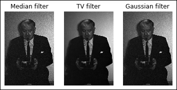
FIGURE 3-2: Different filters for different noise cleaning.
 If you aren't working in IPython (or you aren’t using the magic command
 %matplotlib inline), just close the image when you’ve finished viewing it after filtering noise from the image. (The asterisk in the In [*]: entry in Notebook tells you that the code is still running and you can't move on to the next step.) The act of closing the image ends the code segment.
Manipulating the image
You now have an image in memory and you may want to find out more about it. When you run the following code, you discover the image type and size:
print("data type: %s, dtype: %s, shape: %s" %
(type(image), image.dtype, image.shape))
The output from this call tells you that the image type is a numpy.ndarray, the dtype is uint8, and the image size is 1200 pixels by 800 pixels. The image is actually an array of pixels that you can manipulate in various ways. For example, if you want to crop the image, you can use the following code to manipulate the image array:
image2 = image[100:950,50:700]
plt.imshow(image2, cmap=cm.gray)
plt.show()
print("data type: %s, dtype: %s, shape: %s" %
(type(image2), image2.dtype, image2.shape))
The numpy.ndarray in image2 is smaller than the one in image, so the output is smaller as well. Figure 3-3 shows typical results. Notice that the image is now 850 pixels by 650 pixels in size. The purpose of cropping the image is to make it a specific size. Both images must be the same size for you to analyze them. Cropping is one way to ensure that the images are the correct size for analysis.

FIGURE 3-3: Cropping the image makes it smaller.
Another method that you can use to change the image size is to resize it. The following code resizes the image to a specific size for analysis:
image3 = resize(image2, (600, 460), mode='symmetric')
plt.imshow(image3, cmap=cm.gray)
print("data type: %s, dtype: %s, shape: %s" %
(type(image3), image3.dtype, image3.shape))
The output from the print() function tells you that the image is now 600 pixels by 460 pixels in size. You can compare it to any image with the same dimensions.
After you have cleaned up all the images and made them the right size, you need to flatten them. A dataset row is always a single dimension, not two or more dimensions. The image is currently an array of 600 pixels by 460 pixels, so you can't make it part of a dataset. The following code flattens image3, so it becomes an array of 276,000 elements stored in image_row.
image_row = image3.flatten()
print("data type: %s, shape: %s" %
(type(image_row), image_row.shape))
Notice that the type is still a numpy.ndarray. You can add this array to a dataset and then use the dataset for analysis purposes. The size is 276,000 elements, as anticipated.
Extracting visual features
Machine learning on images works because it can rely on features to compare pictures and associate an image with another one (because of similarity) or to a specific label (guessing, for instance, the represented objects). Humans can easily choose a car or a tree when we see one in a picture. Even if it's the first time that we see a certain kind of tree or car, we can correctly associate it with the right object (labeling) or compare it with similar objects in memory (image recall).
In the case of a car, having wheels, doors, a steering wheel, and so on are all elements that help you categorize a new example of a car among other cars. It happens because you see shapes and elements beyond the image itself; thus, no matter how unusual a tree or a car may be, if it owns certain characteristics, you can $ out what it is.
An algorithm can infer elements (shapes, colors, particulars, relevant elements, and so on) directly from pixels only when you prepare data for it. Apart from special kinds of neural networks, called Convolutional Neural Networks, or CNNs (discussed later in this chapter), it’s always necessary to prepare the right features when working with images. CNNs rank as the state of the art in image recognition because they can extract useful features from raw images by themselves.
Feature preparation from images is like playing with a jigsaw puzzle: You have to figure out any relevant particular, texture, or set of corners represented inside the image to recreate a picture from its details. All this information serves as the image features and makes up a precious element for any machine learning algorithm to complete its job.
CNNs filter information across multiple layers and train the parameters of their convolutions (which are kinds of image filters). In this way, they can filter out the features relevant to the images and the tasks they’re trained to perform and exclude everything else. Other special layers, called pooling layers, help the neural net catch these features in the case of translation (they appear in unusual parts of the image) or rotation.
Applying deep learning requires special techniques and machines that are able to sustain the heavy computational workload. The Caffe library, developed by Yangqing Jia from the Berkeley Vision and Learning Center, allows building such neural networks but also leverages pretrained ones (http://caffe.berkeleyvision.org/model_zoo.html). A pretrained neural network is a CNN trained on a large number of varied images, thus it has learned how to filter out a large variety of features for classification purposes. The pretrained network lets you input your images and obtain a large number of values that correspond to a score on a certain kind of feature previously learned by the network as an output. The features may correspond to a certain shape or texture. What matters to your machine learning objectives is for the most revealing features for your purposes to be among those produced by the pretrained network. Therefore, you must choose the right features by making a selection using another neural network, an SVM, or a simple regression model.
When you can’t use a CNN or pretrained library (because of memory or CPU constraints), OpenCV (https://opencv-python-tutroals.readthedocs.io/en/latest/py_tutorials/py_feature2d/py_table_of_contents_feature2d/py_table_of_contents_feature2d.html) or some Scikit-image functions can still help. For instance, to emphasize the borders of an image, you can apply a simple process using Scikit-image, as shown here:
from skimage import measure
contours = measure.find_contours(image, 0.55)
plt.imshow(image, cmap=cm.gray)
for n, contour in enumerate(contours):
plt.plot(contour[:, 1], contour[:, 0], linewidth=2)
plt.axis('image')
plt.show()
You can read more about finding contours and other algorithms for feature extraction (histograms; corner and blob detection) in the tutorials at https://scikit-image.org/docs/dev/auto_examples/.
Recognizing faces using Eigenfaces
The capability to recognize a face in the crowd has become an essential tool for many professions. For example, both the military and law enforcement rely on it heavily. Of course, facial recognition has uses for security and other needs as well. This example looks at facial recognition in a more general sense. You may have wondered how social networks manage to tag images with the appropriate label or name. The following example demonstrates how to perform this task by creating the right features using eigenfaces.
Eigenfaces is an approach to facial recognition based on the overall appearance of a face, not on its particular details. By means of a technique that can intercept and reshape the variance present in the image, the reshaped information is treated like the DNA of a face, thus allowing the recovery of similar faces (because they have similar variances) in a host of facial images. It’s a less effective technique than extracting features from the details of an image, yet it works, and you can implement it quickly on your computer. This approach demonstrates how machine learning can operate with raw pixels, but it’s more effective when you change image data into another kind of data. You can learn more about eigenfaces at https://towardsdatascience.com/eigenfaces-recovering-humans-from-ghosts-17606c328184 or by trying the tutorial that explores variance decompositions in Scikit-learn at https://scikit-learn.org/stable/auto_examples/decomposition/plot_faces_decomposition.html.
In this example, you use eigenfaces to associate images present in a training set with those in a test set, initially using some simple statistical measures:
import numpy as np
from sklearn.datasets import fetch_olivetti_faces
dataset = fetch_olivetti_faces(shuffle=True,
random_state=101)
train_faces = dataset.data[:350,:]
test_faces = dataset.data[350:,:]
train_answers = dataset.target[:350]
test_answers = dataset.target[350:]
The example begins by using the Olivetti faces dataset, a public domain set of images readily available from Scikit-learn. The following code displays a description of the dataset that you can use to learn more about it:
print (dataset.DESCR)
For this experiment, the code divides the set of labeled images into a training and a test set. You need to pretend that you know the labels of the training set but don’t know anything from the test set. As a result, you want to associate images from the test set to the most similar image from the training set.
The Olivetti dataset consists of 400 photos taken from 40 people (so it contains ten photos of each person). Even though the photos represent the same person, each photo has been taken at different times during the day, with different light and facial expressions or details (for example, with glasses and without). The images are 64 x 64 pixels, so unfolding all the pixels into features creates a dataset made of 400 cases and 4,096 variables. It seems like a high number of features, and actually, it is. Using PCA, as shown in the following code, you can reduce them to a smaller and more manageable number:
from sklearn.decomposition import PCA
n_components = 25
Rpca = PCA(svd_solver='randomized',
n_components=n_components,
whiten=True,
random_state=101).fit(train_faces)
print ('Explained variance by %i components: %0.3f' %
(n_components,
np.sum(Rpca.explained_variance_ratio_)))
compressed_train_faces = Rpca.transform(train_faces)
compressed_test_faces = Rpca.transform(test_faces)
The output from this code tells you about the explained variance of each selected component, based on the number of selected components, which is 25 in this case. If you had used the full set of components, the summed ratio would be 1.0 (or 100 percent).
Explained variance by 25 components: 0.794
The decomposition performed by PCA creates 25 new variables (n_components parameter) and whitening (whiten=True), removing some constant noise (created by textual and photo granularity) and irrelevant information from images in a different way from the filters just discussed. The resulting decomposition uses 25 components, which is about 80 percent of the information held in 4,096 features. The following code displays the effect of this processing:
import matplotlib.pyplot as plt
photo = 17 # This is the photo in the test set
print ('We are looking for face id=%i'
% test_answers[photo])
plt.subplot(1, 2, 1)
plt.axis('off')
plt.title('Unknown face '+str(photo)+' in test set')
plt.imshow(test_faces[photo].reshape(64,64),
cmap=plt.cm.gray, interpolation='nearest')
plt.show()
Figure 3-4 shows the chosen photo, subject number 34, from the test set.
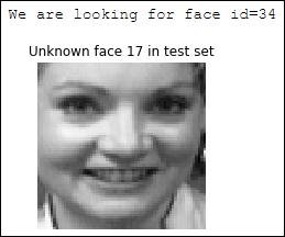
FIGURE 3-4: The example application would like to find similar photos.
After the decomposition of the test set, the example takes the data relative only to photo 17 and subtracts it from the decomposition of the training set. Now the training set is made of differences with respect to the example photo. The code squares them (to remove negative values) and sums them by row, which results in a series of summed errors. The most similar photos are the ones with the least squared errors, that is, the ones whose differences are the least:
#Just the vector of value components of our photo
mask = compressed_test_faces[photo,]
squared_errors = np.sum(
(compressed_train_faces - mask)**2,axis=1)
minimum_error_face = np.argmin(squared_errors)
most_resembling = list(np.where(squared_errors < 20)[0])
print ('Best resembling face in train test: %i' %
train_answers[minimum_error_face])
After running this code, you find the following results:
Best resembling face in train test: 34
As it did before, the code can now display photo 17 using the following code. Photo 17 is the photo that best resembles images from the train set. Figure 3-5 shows typical output from this example.
import matplotlib.pyplot as plt
plt.subplot(2, 2, 1)
plt.axis('off')
plt.title('Unknown face '+str(photo)+' in test set')
plt.imshow(test_faces[photo].reshape(64,64),
cmap=plt.cm.gray, interpolation='nearest')
for k,m in enumerate(most_resembling[:3]):
plt.subplot(2, 2, 2+k)
plt.title('Match in train set no. '+str(m))
plt.axis('off')
plt.imshow(train_faces[m].reshape(64,64),
cmap=plt.cm.gray, interpolation='nearest')
plt.show()
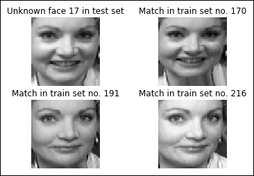
FIGURE 3-5: The output shows the results that resemble the test image.
Even though the most similar photo is quite close to photo 17 (it's just scaled slightly differently), the other two photos are quite different. However, even though those photos don’t match the text image as well, they really do show the same person as in photo 17.
Classifying images
This section adds to your knowledge of facial recognition, this time applying a learning algorithm to a complex set of images, called the Labeled Faces in the Wild dataset, which contains images of famous people collected over the Internet: http://vis-www.cs.umass.edu/lfw/. You must download the dataset from the Internet, using the Scikit-learn package in Python (see the fetch_lfw_people site at https://scikit-learn.org/stable/modules/generated/sklearn.datasets.fetch_lfw_people.html for details). The package mainly contains photos of well-known politicians.
import warnings
warnings.filterwarnings("ignore")
from sklearn.datasets import fetch_lfw_people
lfw_people = fetch_lfw_people(min_faces_per_person=60,
resize=0.4)
X = lfw_people.data
y = lfw_people.target
target_names = [lfw_people.target_names[a] for a in y]
n_samples, h, w = lfw_people.images.shape
from collections import Counter
for name, count in Counter(target_names).items():
print ("%20s %i" % (name, count))
When you run this code, you see some downloading messages. These messages are quite normal, and you shouldn't worry about them. The downloading process can take a while because the dataset is relatively large. When the download process is complete, the example code outputs the name of each well-known politician, along with the number of associated pictures, as shown here:
Colin Powell 236
George W Bush 530
Hugo Chavez 71
Junichiro Koizumi 60
Tony Blair 144
Ariel Sharon 77
Donald Rumsfeld 121
Gerhard Schroeder 109
As an example of dataset variety, after dividing the examples into training and test sets, you can display a sample of pictures from both sets depicting Junichiro Koizumi, former Prime Minister of Japan from 2001 to 2006. Figure 3-6 shows the output of the following code:
from sklearn.cross_validation import
StratifiedShuffleSplit
train, test = list(StratifiedShuffleSplit(target_names,
n_iter=1, test_size=0.1, random_state=101))[0]
plt.subplot(1, 4, 1)
plt.axis('off')
for k,m in enumerate(X[train][y[train]==6][:4]):
plt.subplot(1, 4, 1+k)
if k==0:
plt.title('Train set')
plt.axis('off')
plt.imshow(m.reshape(50,37),
cmap=plt.cm.gray, interpolation='nearest')
plt.show()
for k,m in enumerate(X[test][y[test]==6][:4]):
plt.subplot(1, 4, 1+k)
if k==0:
plt.title('Test set')
plt.axis('off')
plt.imshow(m.reshape(50,37),
cmap=plt.cm.gray, interpolation='nearest')
plt.show()

FIGURE 3-6: Examples from the training and test sets differ in pose and expression.
As you can see, the photos have quite a few variations, even among photos of the same person, which makes the task challenging. The application must consider:
- Expression
- Pose
- Light differences
- Photo quality
For this reason, the example that follows applies the eigenfaces method described in the previous section, using different kinds of decompositions and reducing the initial large vector of pixel features (1850) to a simpler set of 150 features. The example uses PCA, the variance decomposition technique; Non-Negative Matrix Factorization (NMF), a technique for decomposing images into only positive features; and FastICA, an algorithm for Independent Component Analysis, which is an analysis that extracts signals from noise and other separated signals. (This algorithm is successful at handling problems like the cocktail party problem described at https://www.comsol.com/blogs/have-you-heard-about-the-cocktail-party-problem/.)
from sklearn import decomposition
n_components = 50
pca = decomposition.PCA(
svd_solver='randomized',
n_components=n_components,
whiten=True).fit(X[train,:])
nmf = decomposition.NMF(n_components=n_components,
init='nndsvda',
tol=5e-3).fit(X[train,:])
fastica = decomposition.FastICA(n_components=n_components,
whiten=True).fit(X[train,:])
eigenfaces = pca.components_.reshape((n_components, h, w))
X_dec = np.column_stack((pca.transform(X[train,:]),
nmf.transform(X[train,:]),
fastica.transform(X[train,:])))
Xt_dec = np.column_stack((pca.transform(X[test,:]),
nmf.transform(X[test,:]),
fastica.transform(X[test,:])))
y_dec = y[train]
yt_dec = y[test]
After extracting and concatenating the image decompositions into a new training and test set of data examples, the code applies a grid search for the best combinations of parameters for a classification support vector machine (SVM) to perform a correct problem classification:
from sklearn.grid_search import GridSearchCV
from sklearn.svm import SVC
param_grid = {'C': [0.1, 1.0, 10.0, 100.0, 1000.0],
'gamma': [0.0001, 0.001, 0.01, 0.1], }
clf = GridSearchCV(SVC(kernel='rbf'), param_grid)
clf = clf.fit(X_dec, y_dec)
print ("Best parameters: %s" % clf.best_params_)
After the code runs, you see an output showing the best parameters to use, as shown here:
Best parameters: {'C': 10.0, 'gamma': 0.01}
After finding the best parameters, the following code checks for accuracy — that is, the percentage of correct answers in the test set. Obviously, using the preceding code doesn’t pay if the accuracy produced by the SVM is too low; it would be too much like guessing.
from sklearn.metrics import accuracy_score
solution = clf.predict(Xt_dec)
print("Achieved accuracy: %0.3f"
% accuracy_score(yt_dec, solution))
Fortunately, the example provides an estimate of about 0.84 (the measure may change when you run the code on your computer).
Achieved accuracy: 0.837
More interestingly, you can ask for a confusion matrix that shows the correct classes along the rows and the predictions in the columns. When a character in a row has counts in columns different from its row number, the code has mistakenly attributed one of the photos to someone else.
from sklearn.metrics import confusion_matrix
confusion = str(confusion_matrix(yt_dec, solution))
print (' '*26+ ' '.join(map(str,range(8))))
print (' '*26+ '-'*22)
for n, (label, row) in enumerate(
zip(lfw_people.target_names,
                    confusion.split('
'))):
print ('%s %18s > %s' % (n, label, row))
In this case, the example actually gets a perfect score for Junichiro Koizumi (notice that the output shows a 6 in row 6, column 6, and zeros in the remainder of the entries for that row). The code gets most confused about Gerhard Schroeder. Notice that the affected row shows 6 correct entries in column 4, but has a total of 5 incorrect entries in the other columns.
0 1 2 3 4 5 6 7
----------------------
0 Ariel Sharon > [[ 7 0 0 0 1 0 0 0]
1 Colin Powell > [ 0 22 0 2 0 0 0 0]
2 Donald Rumsfeld > [ 0 0 8 2 1 0 0 1]
3 George W Bush > [ 0 1 3 46 1 0 0 2]
4 Gerhard Schroeder > [ 0 0 2 1 6 1 0 1]
5 Hugo Chavez > [ 0 0 0 0 0 6 0 1]
6 Junichiro Koizumi > [ 0 0 0 0 0 0 6 0]
7 Tony Blair > [ 0 0 0 1 1 0 0 12]]
Understanding CNN Image Basics
Digital images are everywhere today because of the pervasive presence of digital cameras, webcams, and mobile phones with cameras. Because capturing images has become so easy, a new, huge stream of data is provided by images. Being able to process images opens the doors to new applications in fields such as robotics, autonomous driving, medicine, security, and surveillance.
Processing an image for use by a computer transforms it into data. Computers send images to a monitor as a data stream composed of pixels, so computer images are best represented as a matrix of pixels values, with each position in the matrix corresponding to a point in the image.
Modern computer images represent colors using a series of 32 bits (8 bits apiece for red, blue, green, and transparency — the alpha channel). You can use just 24 bits to create a true color image, however. The article at http://www.rit-mcsl.org/fairchild/WhyIsColor/Questions/4-5.html explains this process in more detail. Computer images represent color using three overlapping matrices, each one providing information relative to one of three colors: Red, Green, or Blue (also called RGB). Blending different amounts of these three colors enables you to represent any standard human-viewable color, but not those seen by people with extraordinary perception. (Most people can see a maximum of 1,000,000 colors, which is well within the color range of the 16,777,216 colors offered by 24-bit color. Tetrachromats can see 100,000,000 colors, so you couldn’t use a computer to analyze what they see. The article at http://nymag.com/scienceofus/2015/02/what-like-see-a-hundred-million-colors.html tells you more about tetrachromats.)
Generally, an image is therefore manipulated by a computer as a three-dimensional matrix consisting of height, width, and the number of channels — which is three for an RGB image, but could be just one for a black-and-white image. (Grayscale is a special sort of RGB image for which each of the three channels is the same number; see https://introcomputing.org/image-6-grayscale.html for a discussion of how conversions between color and grayscale occur.) With a grayscale image, a single matrix can suffice by having a single number represent the 256-grayscale colors, as demonstrated by the example in Figure 3-7. In that figure, each pixel of an image of a number is quantified by its matrix values.

FIGURE 3-7: Each pixel is read by the computer as a number in a matrix.
Given the fact that images are pixels (represented as numeric inputs), neural network practitioners initially achieved good results by connecting an image directly to a neural network. Each image pixel connected to an input node in the network. Then one or more following hidden layers completed the network, finally resulting in an output layer. The approach worked acceptably for small images and to solve small problems but eventually gave way to different approaches for solving image recognition. As an alternative, researchers used other machine learning algorithms or applied intensive feature creation to transform an image into newly processed data that could help algorithms recognize the image better. An example of image feature creation is the Histograms of Oriented Gradients (HOG), which is a computational way to detect patterns in an image and turn them into a numeric matrix. (You can explore how HOG works by viewing this tutorial from the Skimage package: https://scikit-image.org/docs/dev/auto_examples/features_detection/plot_hog.html.)
Neural network practitioners found image feature creation to be computationally intensive and often impractical. Connecting image pixels to neurons was difficult because it required computing an incredibly large number of parameters, and the network couldn’t achieve translation invariance, which is the capability to decipher a represented object under different conditions of size, distortion, or position in the image, as shown in Figure 3-8.
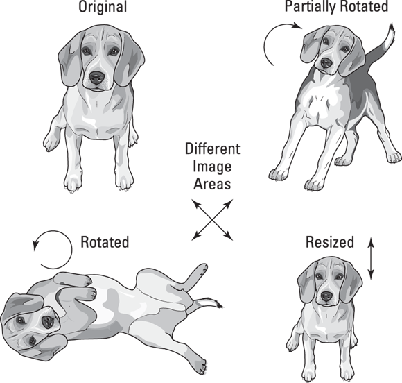
FIGURE 3-8: Only by translation invariance can an algorithm spot the dog and its variations.
A neural network, which is made of dense layers, as described in the previous chapters in this minibook, can detect only images that are similar to those used for training — those that it has seen before — because it learns by spotting patterns at certain image locations. Also, a neural network can make many mistakes. Transforming an image before feeding it to the neural network can partially solve the problem by resizing, moving, cleaning the pixels, and creating special chunks of information for better network processing. This technique, called feature creation, requires expertise on the necessary image transformations, as well as many computations in terms of data analysis. Because of the intense level of custom work required, image recognition tasks are more the work of an artisan than a scientist. However, the amount of custom work has decreased over time as the base of libraries automating certain tasks has increased.
Moving to CNNs with Character Recognition
CNNs aren’t a new idea. They appeared at the end of the 1980s as the solution for character recognition problems. Yann LeCun devised CNNs when he worked at AT&T Labs Research, together with other scientists such as Yoshua Bengio, Leon Bottou, and Patrick Haffner, on a network named LeNet5.
At one time, people used Support Vector Machines (SVMs) to perform character recognition. However, SVMs were problematic in that they need to model each pixel as a feature. Consequently, they fail to correctly predict the right character when the input varies greatly from the character set used for training. CNNs avoid this problem by generalizing what they learn, so predicting the correct character is possible even when the training character sets differ in some significant way. Of course, this is the short explanation as to why this section uses a CNN rather than an SVM to perform character recognition. You can find a much more detailed explanation at https://medium.com/analytics-vidhya/the-scuffle-between-two-algorithms-neural-network-vs-support-vector-machine-16abe0eb4181.
This example relies on the Modified National Institute of Standards and Technology (MNIST) (http://yann.lecun.com/exdb/mnist/) dataset that contains a training set of 60,000 examples and a test set of 10,000 examples. The dataset was originally taken from National Institute of Standards and Technology (NIST) (https://www.nist.gov/) documents. You can find a detailed description of the dataset’s construction on the MNIST site.
Accessing the dataset
The first step is to obtain access to the MNIST dataset. The following code downloads the dataset and then displays a series of characters from it, as shown in Figure 3-9:
import matplotlib.pyplot as plt
%matplotlib inline
from keras.datasets import mnist
(X_train, y_train), (X_test, y_test) = mnist.load_data()
plt.plot()
plt.axis('off')
for k, m in enumerate(X_train[:4]):
plt.subplot(1, 4, 1+k)
plt.axis('off')
plt.imshow(m, cmap=plt.cm.gray)
plt.show()

FIGURE 3-9: Displaying some of the handwritten characters from MNIST.
Reshaping the dataset
Each of the 60,000 images in X_train and the 10,000 images in X_test are 28 pixels by 28 pixels. In the “Manipulating the image” section, earlier in this chapter, you see how to flatten a single image using the numpy.ndarray.flatten (https://docs.scipy.org/doc/numpy-1.15.0/reference/generated/numpy.ndarray.flatten.html). This time, you rely on numpy.reshape (https://docs.scipy.org/doc/numpy/reference/generated/numpy.reshape.html) to perform the same task. To obtain the required output, you must supply the number of entries and the number of pixels, as shown here:
import numpy
from keras.utils import np_utils
numpy.random.seed(100)
pixels = X_train.shape[1] * X_train.shape[2]
train_entries = X_train.shape[0]
test_entries = X_test.shape[0]
X_train_row = X_train.reshape(train_entries, pixels)
X_test_row = X_test.reshape(test_entries, pixels)
print(X_train_row.shape)
print(X_test_row.shape)
The output of this part of the code is
(60000, 784)
(10000, 784)
Now that the individual entries are flattened rather than 2-D, you can normalize them. Normalization takes the 255 shades of gray and turns them into values between 0 and 1. However, the dtype of the X_train_row and X_test_row rows is currently unit8. What you really need is a float32, so this next step performs the required conversion as well:
# Change the data type
X_train_row = X_train_row.astype('float32')
X_test_row = X_test_row.astype('float32')
# Perform the normalization.
X_train_row = X_train_row / 255
X_test_row = X_test_row / 255
Encoding the categories
In the preceding sections, you're essentially asking the CNN to choose from ten different categories for each of the entries in X_train_row and X_test_row because the output can be from 0 through 9. This example uses a technique called one-hot encoding (https://hackernoon.com/what-is-one-hot-encoding-why-and-when-do-you-have-to-use-it-e3c6186d008f). When you start, the values in y_train and y_test range from 0 through 9. The problem with this approach is that the learning process will associate the value 9 as being a lot better than the value 0, even though it doesn't matter. So, this process converts a single scalar value, such as 7, into a binary vector. The following code shows how this works:
y_train_cat = np_utils.to_categorical(y_train)
y_test_cat = np_utils.to_categorical(y_test)
num_classes = y_test_cat.shape[1]
print(num_classes)
print(y_test[0])
print(y_test_cat[0])
When you run this code, you get this output:
10
7
[0. 0. 0. 0. 0. 0. 0. 1. 0. 0.]
The number of classes is still the same at 10. The original value of the first entry in y_test is 7. However, the encoding process turns it into the vector shown next, where the eighth value, which equates to 7 (when starting with 0), is set to 1 (or True). By encoding the entries this way, you preserve the label, 7, without giving the label any special weight.
Defining the model
In this section, you define a model to use to perform the analysis referred to in the preceding sections. A model starts with a framework of sorts and you then add layers to the model. Each layer performs a certain type of processing based on the attributes you set for it. After you create the model and define its layers, you then compile the model so that the application can use it, as shown here:
from keras.models import Sequential
from keras.layers import Dense
from keras.layers import Dropout
def baseline_model():
# Specify which model to use.
model = Sequential()
# Add layers to the model.
model.add(Dense(pixels, input_dim=pixels,
kernel_initializer='normal',
activation='relu'))
model.add(Dense(num_classes,
kernel_initializer='normal',
activation='softmax'))
# Compile the model
model.compile(loss='categorical_crossentropy',
optimizer='adam', metrics=['accuracy'])
return model
The Sequential model (explained at https://keras.io/models/sequential/ and https://keras.io/getting-started/sequential-model-guide/) provides the means to create a linear stack of layers. To add layers to this model, you simply call add(). The two layers used in this example are ReLU and softmax. Book 4, Chapters 2 and 3, respectively, give all the information you need to understand both of these layers and what they do. The final task is to compile the model so that you can use it to perform useful work.
Using the model
The final step in this process is to use the model to perform an analysis of the data. The following code actually creates a model using the definition from the previous section. It then fits this model to the data. When the training part of the process is complete, the code can evaluate the success or failure of the model in detecting the correct values for each handwritten character:
model = baseline_model()
model.fit(X_train_row, y_train_cat,
validation_data=(X_test_row, y_test_cat),
epochs=10, batch_size=200, verbose=2)
scores = model.evaluate(X_test_row, y_test_cat, verbose=0)
print("Baseline Error: %.2f%%" % (100-scores[1]*100))
The output tells you that the model works well but doesn't provide absolute reliability. The model has a 1.87 percent chance of choosing the wrong character, as shown here:
Train on 60000 samples, validate on 10000 samples
Epoch 1/10
- 13s - loss: 0.2800 - acc: 0.9205 - val_loss: 0.1344
- val_acc: 0.9623
Epoch 2/10
- 13s - loss: 0.1116 - acc: 0.9681 - val_loss: 0.0916
- val_acc: 0.9722
Epoch 3/10
- 12s - loss: 0.0716 - acc: 0.9794 - val_loss: 0.0730
- val_acc: 0.9775
Epoch 4/10
- 12s - loss: 0.0501 - acc: 0.9854 - val_loss: 0.0677
- val_acc: 0.9776
Epoch 5/10
- 12s - loss: 0.0360 - acc: 0.9902 - val_loss: 0.0615
- val_acc: 0.9812
Epoch 6/10
- 12s - loss: 0.0264 - acc: 0.9929 - val_loss: 0.0643
- val_acc: 0.9794
Epoch 7/10
- 12s - loss: 0.0188 - acc: 0.9957 - val_loss: 0.0616
- val_acc: 0.9802
Epoch 8/10
- 12s - loss: 0.0144 - acc: 0.9967 - val_loss: 0.0609
- val_acc: 0.9811
Epoch 9/10
- 12s - loss: 0.0106 - acc: 0.9978 - val_loss: 0.0614
- val_acc: 0.9820
Epoch 10/10
- 13s - loss: 0.0087 - acc: 0.9980 - val_loss: 0.0587
- val_acc: 0.9813
Baseline Error: 1.87%
Explaining How Convolutions Work
Convolutions easily solve the problem of translation invariance because they offer a different image-processing approach inside the neural network. The idea started from a biological point of view by observing what happens in the human visual cortex.
A 1962 experiment by Nobel Prize winners David Hunter Hubel and Torsten Wiesel demonstrated that only certain neurons activate in the brain when the eye sees certain patterns, such as horizontal, vertical, or diagonal edges. In addition, the two scientists found that the neurons organize vertically, in a hierarchy, suggesting that visual perception relies on the organized contribution of many single, specialized neurons. (You can find out more about this experiment by reading the article at https://knowingneurons.com/2014/10/29/hubel-and-wiesel-the-neural-basis-of-visual-perception/.) Convolutions simply take this idea and, by using mathematics, apply it to image processing in order to enhance the capabilities of a neural network to recognize different images accurately.
Understanding convolutions
To understand how convolutions work, you start from the input. The input is an image composed of one or more pixel layers, called channels, and the image uses values ranging from 0–255, with 0 meaning that the individual pixel is fully switched off and 255 meaning that the individual pixel is switched on. (Usually, the values are stored as integers to save memory.) As mentioned in the preceding section of this chapter, RGB images have individual channels for red, green, and blue colors. Mixing these channels generates the palette of colors as you see them on the screen.
A convolution works by operating on small image chunks across all image channels simultaneously. (Picture a slice of layer cake, with each piece showing all the layers). Image chunks are simply a moving image window: The convolution window can be a square or a rectangle, and it starts from the upper left of the image and moves from left to right and from top to bottom. The complete tour of the window over the image is called a filter and implies a complete transformation of the image. Also important to note is that when a new chunk is framed by the window, the window then shifts a certain number of pixels; the amount of the slide is called a stride. A stride of 1 means that the window is moving one pixel toward right or bottom; a stride of 2 implies a movement of two pixels; and so on.
Every time the convolution window moves to a new position, a filtering process occurs to create part of the filter described in the previous paragraph. In this process, the values in the convolution window are multiplied by the values in the kernel. (A kernel is a small matrix used for blurring, sharpening, embossing, edge detection, and more. You choose the kernel you need for the task in question. The article at http://setosa.io/ev/image-kernels/ tells you more about various kernel types.) The kernel is the same size as the convolution window. Multiplying each part of the image with the kernel creates a new value for each pixel, which in a sense is a new, processed feature of the image. The convolution outputs the pixel value and when the sliding window has completed its tour across the image, you have filtered the image. As a result of the convolution, you find a new image having the following characteristics:
- If you use a single filtering process, the result is a transformed image of a single channel.
- If you use multiple kernels, the new image has as many channels as the number of filters, each one containing specially processed new feature values. The number of filters is the filter depth of a convolution.
- If you use a stride of 1, you get an image of the same dimensions as the original.
- If you use strides of a size above 1, the resulting convoluted image is smaller than the original (a stride of size two implies halving the image size).
- The resulting image may be smaller depending on the kernel size, because the kernel has to start and finish its tour on the image borders. When processing the image, a kernel will eat up its size minus one. For instance, a kernel of 3 x 3 pixels processing a 7-x-7 pixel image will eat up 2 pixels from the height and width of the image, and the result of the convolution will be an output of size 5 x 5 pixels. You have the option to pad the image with zeros at the border (meaning, in essence, to put a black border on the image) so that the convolution process won’t reduce the final output size. This strategy is called same padding. If you just let the kernel reduce the size of your starting image, it’s called valid padding.
Image processing has relied on the convolution process for a long time. Convolution filters can detect an edge or enhance certain characteristics of an image. Figure 3-10 provides an example of some convolutions transforming an image.

FIGURE 3-10: A convolution processes a chunk of an image by matrix multiplication.
The problem with using convolutions is that they are human made and require effort to figure out. When using a neural network convolution instead, you just set:
- The number of filters (the number of kernels operating on an image that is its output channels)
- The kernel size (set just one side for a square; set width and height for a rectangle)
- The strides (usually 1- or 2-pixel steps)
- Whether you want the image black bordered (choose valid padding or same padding)
After determining the image-processing parameters, the optimization process determines the kernel values used to process the image in a way to allow the best classification of the final output layer. Each kernel matrix element is therefore a neural network neuron and modified during training using backpropagation for the best performance of the network itself.
Another interesting aspect of this process is that each kernel specializes in finding specific aspects of an image. For example, a kernel specialized in filtering features typical of cats can find a cat no matter where it is in an image and, if you use enough kernels, every possible variant of an image of a kind (resized, rotated, translated) is detected, rendering your neural network an efficient tool for image classification and recognition.
In Figure 3-11, the borders of an image are easily detected after a 3-x-3 pixel kernel is applied. This kernel specializes in finding edges, but another kernel could spot different image features. By changing the values in the kernel, as the neural network does during backpropagation, the network finds the best way to process images for its regression or classification purpose.
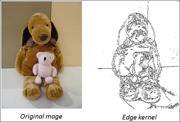
FIGURE 3-11: The borders of an image are detected after applying a 3-x-3 pixel kernel.
 The kernel is a matrix whose values are defined by the neural network optimization, multiplied by a small patch of the same size moving across the image, but it can be intended as a neural layer whose weights are shared across the different input neurons. You can see the patch as an immobile neural layer connected to the many parts of the image always using the same set of weights. It is exactly the same result.
Keras offers a convolutional layer, Conv2D, out of the box. This Keras layer can take both the input directly from the image (in a tuple, you have to set the input_shape the width, height, and number of channels of your image) or from another layer (such as another convolution). You can also set filters, kernel_size, strides, and padding, which are the basic parameters for any convolutional layers, as described earlier in the chapter.
When setting a Conv2D layer, you may also set many other parameters, which are actually a bit too technical and may not be necessary for your first experiments with CNNs. The only other parameters you may find useful now are activation, which can add an activation of your choice, and name, which sets a name for the layer.
Simplifying the use of pooling
Convolutional layers transform the original image using various kinds of filtering. Each layer finds specific patterns in the image (particular sets of shapes and colors that make the image recognizable). As this process continues, the complexity of the neural network grows because the number of parameters grows as the network gains more filters. To keep the complexity manageable, you need to speed the filtering and reduce the number of operations.
Pooling layers can simplify the output received from convolutional layers, thus reducing the number of successive operations performed and using fewer convolutional operations to perform filtering. Working in a fashion similar to convolutions (using a window size for the filter and a stride to slide it), pooling layers operate on patches of the input they receive and reduce a patch to a single number, thus effectively downsizing the data flowing through the neural network.
Figure 3-12 represents the operations done by a pooling layer. The pooling layer receives the filtered data, represented by the left 4-x-4 matrix, as input and operates on it using a window of size 2 pixels that moves by a stride of 2 pixels. As a result, the pooling layer produces the right output: a 2-x-2 matrix. The network applies the pooling operation on four patches represented by four different colored parts of the matrix. For each patch, the pooling layer computes the maximum value and saves it as an output.

FIGURE 3-12: A max pooling layer operating on chunks of a reduced image.
The current example relies on the max pooling layer because it uses the max transformation on its sliding window. You actually have access to four principal types of pooling layers:
- Max pooling
- Average pooling
- Global max pooling
- Global average pooling
In addition, these four pooling layer types have different versions, depending on the dimensionality of the input they can process:
- 1-D pooling: Works on vectors. Thus, 1-D pooling is ideal for sequence data such as temporal data (data representing events following each other in time) or text (represented as sequences of letters or words). It takes the maximum or the average of contiguous parts of the sequence.
- 2-D pooling: Fits spatial data that fits a matrix. You can use 2-D pooling for a grayscale image or each channel of an RBG image separately. It takes the maximum or the average of small patches (squares) of the data.
- 3-D pooling: Fits spatial data represented as spatial-temporal data. You could use 3-D pooling for images taken across time. A typical example is to use magnetic resonance imaging (MRI) for a medical examination. Radiologists use an MRI to examine body tissues with magnetic fields and radio waves. (See the article from Stanford AI for healthcare to learn more about the contribution of deep learning:
https://medium.com/stanford-ai-for-healthcare/dont-just-scan-this-deep-learning-techniques-for-mri-52610e9b7a85.) This kind of pooling takes the maximum or the average of small chunks (cubes) from the data.
You can find all these layers described in the Keras documentation, together with all their parameters, at https://keras.io/layers/pooling/.
Describing the LeNet architecture
You may have been amazed by the description of a CNN in the preceding section, and about how its layers (convolutions and max pooling) work, but you may be even more amazed at discovering that it's not a new technology; instead, it appeared in the 1990s. The following sections describe the LeNet architecture in more detail.
Considering the underlying functionality
The key person behind this innovation was Yann LeCun, who was working at AT&T Labs Research as head of the Image Processing Research Department. LeCun specialized in optical character recognition and computer vision. Yann LeCun is a French computer scientist who created CNNs with Léon Bottou, Yoshua Bengio, and Patrick Haffner. At present, he is the Chief AI Scientist at Facebook AI Research (FAIR) and a Silver Professor at New York University (mainly affiliated with the NYU Center for Data Science). His personal home page is at http://yann.lecun.com/.
In the late 1990s, AT&T implemented LeCun’s LeNet5 to read ZIP codes for the United States Postal Service. The company also used LeNet5 for ATM check readers, which can automatically read the check amount. The system doesn’t fail, as reported by LeCunn at https://pafnuty.wordpress.com/2009/06/13/yann-lecun/. However, the success of the LeNet passed almost unnoticed at the time because the AI sector was undergoing an AI winter: Both the public and investors were significantly less interested and attentive to improvements in neural technology than they are now.
Part of the reason for an AI winter was that many researchers and investors lost faith in the idea that neural networks would revolutionize AI. Data of the time lacked the complexity for such a network to perform well. (ATMs and the USPS were notable exceptions because of the quantities of data they handled.) With a lack of data, convolutions only marginally outperform regular neural networks made of connected layers. In addition, many researchers achieved results comparable to LeNet5 using brand-new machine learning algorithms such as Support Vector Machines (SVMs) and Random Forests, which were algorithms based on mathematical principles different from those used for neural networks.
You can see the network in action at http://yann.lecun.com/exdb/lenet/ or in this video, in which a younger LeCun demonstrates an earlier version of the network: https://www.youtube.com/watch?v=FwFduRA_L6Q. At that time, having a machine able to decipher both typewritten and handwritten numbers was quite a feat.
As shown in Figure 3-13, the LeNet5 architecture consists of two sequences of convolutional and average pooling layers that perform image processing. The last layer of the sequence is then flattened; that is, each neuron in the resulting series of convoluted 2-D arrays is copied into a single line of neurons. At this point, two fully connected layers and a softmax classifier complete the network and provide the output in terms of probability. The LeNet5 network is really the basis of all the CNNs that follow. Re-creating the architecture using Keras, as you can do in the following sections, will explain it layer-by-layer and demonstrate how to build your own convolutional networks.

FIGURE 3-13: The architecture of LeNet5, a neural network for handwritten digits recognition.
Building your own LeNet5 network
This network will be trained on a relevant amount of data (the digits dataset provided by Keras, consisting of more than 60,000 examples). You could therefore have an advantage if you run it on Colab, or on your local machine if you have a GPU available. After opening a new notebook, you start by importing the necessary packages and functions from Keras using the following code (note that some of this code is a repeat from the “Moving to CNNs with Character Recognition” section, earlier in this chapter):
import keras
import numpy as np
from keras.datasets import mnist
from keras.models import Sequential
from keras.layers import Conv2D, AveragePooling2D
from keras.layers import Dense, Flatten
from keras.losses import categorical_crossentropy
After importing the necessary tools, you need to collect the data:
(X_train, y_train), (X_test, y_test) = mnist.load_data()
The first time you execute this command, the mnist command will download all the data from the Internet, which could take a while. The downloaded data consists of single-channel 28-x-28-pixel images representing handwritten numbers from zero to nine. As a first step, you need to convert the response variable (y_train for the training phase and y_test for the test after the model is completed) into something that the neural network can understand and work on:
num_classes = len(np.unique(y_train))
print(y_train[0], end=' => ')
y_train = keras.utils.to_categorical(y_train, 10)
y_test = keras.utils.to_categorical(y_test, 10)
print(y_train[0])
This code snippet translates the response from numbers to vectors of numbers, where the value at the position corresponding to the number the network will guess is 1 and the others are 0. The code will also output the transformation for the first image example in the training set:
5 => [0. 0. 0. 0. 0. 1. 0. 0. 0. 0.]
Notice that the output is 0 based and that the 1 appears at the position corresponding to the number 5. This setting is used because the neural network needs a response layer, which is a set of neurons (hence the vector) that should become activated if the provided answer is correct. In this case, you see ten neurons, and in the training phase, the code activates the correct answer (the value at the correct position is set to 1) and turns the others off (their values are 0). In the test phase, the neural network uses its database of examples to turn the correct neuron on, or at least turn on more than the correct one. In the following code, the code prepares the training and test data:
X_train = X_train.astype(np.float32) / 255
X_test = X_test.astype(np.float32) / 255
img_rows, img_cols = X_train.shape[1:]
X_train = X_train.reshape(len(X_train),
img_rows, img_cols, 1)
X_test = X_test.reshape(len(X_test),
img_rows, img_cols, 1)
input_shape = (img_rows, img_cols, 1)
The pixel numbers, which range from 0 to 255, are transformed into a decimal value ranging from 0 to 1. The first two lines of code optimize the network to work properly with large numbers that could cause problems. The lines that follow reshape the images to have height, width, and channels.
The following line of code defines the LeNet5 architecture. You start by calling the sequential function that provides an empty model:
lenet = Sequential()
The first layer added is a convolutional layer, named C1:
lenet.add(Conv2D(6, kernel_size=(5, 5), activation='tanh',
input_shape=input_shape, padding='same', name='C1'))
The convolution operates with a filter size of 6 (meaning that it will create six new channels made by convolutions) and a kernel size of 5 x 5 pixels.
The activation for all the layers of the network but the last one is tanh (Hyperbolic Tangent function), a nonlinear function that was state of the art for activation at the time Yann LeCun created LetNet5. The function is outdated today, but the example uses it to build a network that resembles the original LetNet5 architecture. To use such a network for your own projects, you should replace it with a modern ReLU (see https://www.kaggle.com/dansbecker/rectified-linear-units-relu-in-deep-learning for details). The example adds a pooling layer, named S2, which uses a 2-x-2-pixel kernel:
lenet.add(AveragePooling2D(
pool_size=(2, 2), strides=(1, 1), padding='valid'))
At this point, the code proceeds with the sequence, always performed with a convolution and a pooling layer but this time using more filters:
lenet.add(Conv2D(16, kernel_size=(5, 5), strides=(1, 1),
activation='tanh', padding='valid'))
lenet.add(AveragePooling2D(
pool_size=(2, 2), strides=(1, 1), padding='valid'))
The LeNet5 closes incrementally using a convolution with 120 filters. This convolution doesn't have a pooling layer but rather a flattening layer, which projects the neurons into the last convolution layer as a dense layer:
lenet.add(Conv2D(120, kernel_size=(5, 5),
activation='tanh', name='C5'))
lenet.add(Flatten())
The closing of the network is a sequence of two dense layers that process the convolution’s outputs using the tanh and softmax activation. These two layers provide the final output layers where the neurons activate an output to signal the predicted answer. The softmax layer is actually the output layer, as specified by name='OUTPUT':
lenet.add(Dense(84, activation='tanh', name='FC6'))
lenet.add(Dense(10, activation='softmax', name='OUTPUT'))
When the network is ready, you need Keras to compile it. (Behind all the Python code is some C language code.) Keras compiles it based on the SGD optimizer:
lenet.compile(loss=categorical_crossentropy,
optimizer='SGD', metrics=['accuracy'])
lenet.summary()
The summary tells you about the structure of your model:
Layer (type) Output Shape Param #
==========================================================
C1 (Conv2D) (None, 28, 28, 6) 156
__________________________________________________________
average_pooling2d_1 (Average (None, 27, 27, 6) 0
__________________________________________________________
conv2d_1 (Conv2D) (None, 23, 23, 16) 2416
__________________________________________________________
average_pooling2d_2 (Average (None, 22, 22, 16) 0
__________________________________________________________
C5 (Conv2D) (None, 18, 18, 120) 48120
__________________________________________________________
flatten_1 (Flatten) (None, 38880) 0
__________________________________________________________
FC6 (Dense) (None, 84) 3266004
__________________________________________________________
OUTPUT (Dense) (None, 10) 850
==========================================================
Total params: 3,317,546
Trainable params: 3,317,546
Non-trainable params: 0
__________________________________________________________
At this point, you can run the network and wait for it to process the images:
batch_size = 64
epochs = 50
history = lenet.fit(X_train, y_train,
batch_size=batch_size,
epochs=epochs,
validation_data=(X_test,
y_test))
Completing the run takes 50 epochs, with each epoch processing batches of 64 images at one time. (An epoch is the passing of the entire dataset through the neural network one time, and a batch is a part of the dataset, which means breaking the dataset into 64 chunks in this case.) With each epoch (lasting about eight seconds if you use Colab), you can monitor a progress bar telling you the time required to complete that epoch. You can also read the accuracy measures for both the training set (the optimistic estimate of the goodness of your model; see https://towardsdatascience.com/measuring-model-goodness-part-1-a24ed4d62f71 for details on what, precisely, goodness means) and the test set (the more realistic view). At the last epoch, you should read that a LeNet5 built in a few steps achieves an accuracy of 0.988, meaning that out every 100 handwritten numbers that it tries to recognize, the network should guess about 99 correctly. To see this number more clearly, you use the following code:
print("Best validation accuracy: {:0.3f}"
.format(np.max(history.history['val_acc'])))
You can also create a plot of how the training process went using this code:
plt.plot(history.history['acc'])
plt.plot(history.history['val_acc'])
plt.ylabel('accuracy'); plt.xlabel('epochs')
plt.legend(['train', 'test'], loc='lower right')
plt.show()
Figure 3-14 shows typical output for the plotting process.
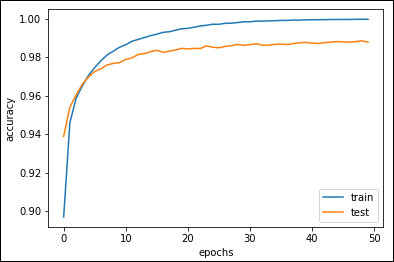
FIGURE 3-14: A plot of the LeNet5 network training process.
Detecting Edges and Shapes from Images
Convolutions process images automatically and perform better than a densely connected layer because they learn image patterns at a local level and can retrace them in any other part of the image (a characteristic called translation invariance). On the other hand, traditional dense neural layers can determine the overall characteristics of an image in a rigid way without the benefit of translation invariance. The difference between convolutions and tradition layers is like that between learning a book by memorizing the text in meaningful chunks or memorizing it word by word. The student (or the convolutions) who learned chunk by chunk can better abstract the book content and is ready to apply that knowledge to similar cases. The student (or the dense layer) who learned it word by word struggles to extract something useful.
CNNs are not magic, nor are they a black box. You can understand them through image processing and leverage their functionality to extend their capabilities to new problems. This feature helps solve a series of computer vision problems that data scientists deemed too hard to crack using older strategies.
Visualizing convolutions
A CNN uses different layers to perform specific tasks in a hierarchical way. Yann LeCun (see the “Moving to CNNs with Character Recognition” section, earlier in this chapter) noticed how LeNet first processed edges and contours, and then motifs, and then categories, and finally objects. Recent studies further unveil how convolutions really work:
- Initial layers: Discover the image edges
- Middle layers: Detect complex shapes (created by edges)
- Final layers: Uncover distinctive image features that are characteristic of the image type that you want the network to classify (for instance, the nose of a dog or the ears of a cat)
This hierarchy of patterns discovered by convolutions also explains why deep convolutional networks perform better than shallow ones: The more stacked convolutions there are, the better the network can learn more and more complex and useful patterns for successful image recognition. Figure 3-15 provides an idea of how things work. The image of a dog is processed by convolutions, and the first layer grasps patterns. The second layer accepts these patterns and assembles them into a dog. If the patterns processed by the first layer seem too general to be of any use, the patterns unveiled by the second layer recreate more characteristic dog features that provide an advantage to the neural network in recognizing dogs.
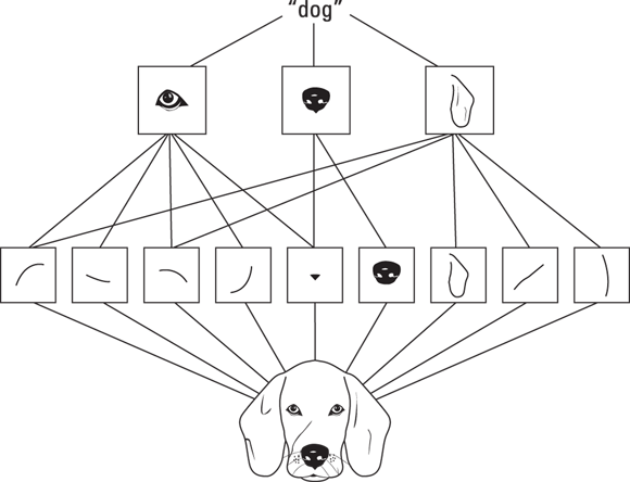
FIGURE 3-15: Processing a dog image using convolutions.
The difficulty in determining how a convolution works is in understanding how the kernel (matrix of numbers) creates the convolutions and how they work on image patches. When you have many convolutions working one after the other, determining the result through direct analysis is difficult. However, a technique designed for understanding such networks builds images that activate the most convolutions. When an image strongly activates a certain layer, you have an idea of what that layer perceives the most.
Analyzing convolutions helps you understand how things work, both to avoid bias in prediction and to devise new ways to process images. For instance, you may discover that your CNN is distinguishing dogs from cats by activating on the background of the image because the images you used for the training represents dogs outdoors and cats indoors.
A 2017 paper called “Feature Visualization,” by Chris Olah, Alexander Mordvintsev, and Ludwig Schubert from the Google Research and Google Brain Team, explains this process in detail (https://distill.pub/2017/feature-visualization/). You can even inspect the images yourself by clicking and pointing at the layers of GoogleLeNet, a CNN built by Google at https://distill.pub/2017/feature-visualization/appendix/. The images from the Feature Visualization may remind you of deepdream images, if you had occasion to see some when they were a hit on the web (read the original deepdream paper and glance at some images at https://ai.googleblog.com/2015/06/inceptionism-going-deeper-into-neural.html). Feature Visualization is the same technique as deepdream, but instead of looking for images that activate a layer the most, you pick a convolutional layer and let it transform an image.
You can also copy the style of works from a great artist of the past, such as Picasso or Van Gogh, using a similar technique that's based on using convolutions to transform an existing image; this technique is a process called artistic style transfer. The resulting picture is modern, but the style isn’t. You can get some interesting examples of artistic style transfer from the original paper “A Neural Algorithm of Artistic Style,” by Leon Gatys, Alexander Ecker, and Matthias Bethge (found at https://arxiv.org/pdf/1508.06576.pdf).
In Figure 3-16, the original image is transformed in style by applying the drawing and color characteristics found in the Japanese Ukiyo-e “The Great Wave off Kanagawa,” a woodblock print by the Japanese artist Katsushika Hokusai, who lived from 1760 to 1849.

FIGURE 3-16: The content of an image is transformed by style transfer.
Unveiling successful architectures
In recent years, data scientists have achieved great progress thanks to deeper investigation into how CNNs work. Other methods have also added to the progress in understanding how CNNs work. Image competitions have played a major role by challenging researchers to improve their networks, which has made large quantities of images available.
The architecture update process started during the last AI winter. Fei-Fei Li, a computer science professor at the University of Illinois at Urbana Champaign (and now chief scientist at Google Cloud as well as professor at Stanford) decided to provide more real-world datasets to better test algorithms for neural networks. She started amassing an incredible number of images representing a large number of object classes. She and her team performed such a huge task by using Amazon’s Mechanical Turk, a service that you use to ask people to do microtasks for you (such as classifying an image) for a small fee.
The resulting dataset, completed in 2009, was called ImageNet and initially contained 3.2 million labeled images (it now contains more than 10 million images) arranged into 5,247 hierarchically organized categories. If interested, you can explore the dataset at http://www.image-net.org/ or read the original paper at http://www.image-net.org/papers/imagenet_cvpr09.pdf.
ImageNet soon appeared at a 2010 competition in which neural networks, using convolutions (hence the revival and further development of the technology developed by Yann LeCun in the 1990s), proved their capability in correctly classifying images arranged into 1,000 classes. In seven years of competition (the challenge closed in 2017), the winning algorithms improved the accuracy of predicting images from 71.8 percent to 97.3 percent, which surpasses human capabilities. (Humans make mistakes in classifying objects.) Here are some notable CNN architectures that were devised for the competition:
- AlexNet (2012): Created by Alex Krizhevsky from the University of Toronto. It used CNNs with an 11-x-11-pixel filter, won the competition, and introduced the use of GPUs for training neural networks, together with the ReLU activation to control overfitting.
- VGGNet (2014): This appeared in two versions, 16 and 19. It was created by the Visual Geometry Group at Oxford University and defined a new 3-x-3 standard in filter size for CNNs.
- ResNet (2015): Created by Microsoft. This CNN not only extended the idea of different versions of the network (50, 101, 152) but also introduced skip layers, a way to connect deeper layers with shallower ones to prevent the vanishing gradient problem and allow much deeper networks that are more capable of recognizing patterns in images.
You can take advantage of all the innovations introduced by the ImageNet competition and even use each of the neural networks. This accessibility allows you to replicate the network performance seen in the competitions and successfully extend them to myriad other problems.
Discussing transfer learning
Networks that distinguish objects and correctly classify them require a lot of images, a long processing time, and vast computational capacity to learn what to do. Adapting a network’s capability to new image types that weren’t part of the initial training means transferring existing knowledge to the new problem. This process of adapting a network’s capability is called transfer learning, and the network you are adapting is often referred to as a pretrained network. You can’t apply transfer learning to other machine learning algorithms; only deep learning has the capability of transferring what it learned with one problem to another.
Transfer learning is something new to most machine learning algorithms and opens a possible market for transferring knowledge from one application to another, and from one company to another. Google is already doing that; it is sharing its immense data repository by making public the networks it built on TF Hub (https://www.tensorflow.org/hub).
For instance, you can transfer a network that’s capable of distinguishing between dogs and cats to perform a job that involves spotting dishes of macaroni and cheese. From a technical point of view, you achieve this task in different ways, depending on how similar the new image problem is to the previous one and how many new images you have for training. (A small image dataset amounts to a few thousand images, and sometimes even fewer.)
If your new image problem is similar to the old one, your network may know all the convolutions necessary (edge, shape, and high-level feature layers) to decipher similar images and classify them. In this case, you don’t need to put too many images into training, add much computational power, or adapt your pretrained network too deeply. This type of transfer is the most common application of transfer learning, and you usually apply it by leveraging a network trained during the ImageNet competition (because those networks were trained on so many images that you probably have all the convolutions needed to transfer the knowledge to other tasks).
Say that the task you want to extend involves not only spotting dogs in images but also determining the dog’s breed. You use the majority of the layers of an ImageNet network such as VGG16 as they are, without further adjustment. In transfer learning, you freeze the values of the pretrained coefficients of the convolutions so that they are not affected by any further training and the network won’t overfit to the data you have, if it is too little. (You can see overfitting discussed in the “Checking the fit using R2” section of Book 3, Chapter 1.)
With the new images, you then train the output layers set on the new problem (a process known as fine-tuning). In a short time and with just a few examples, the network will apply what it learned in distinguishing dogs and cats to breeds of dogs. It will perform even better than a neural network trained only to recognize breeds of dogs because in fine-tuning, it is leveraging what the network has learned before from millions of images.
A neural network identifies only objects that it has been trained to identify. Consequently, if you train a CNN to recognize major breeds of dogs such as a Labrador Retriever or a Husky, the CNN won’t recognize mixes of those two breeds, such as a Labsky. Instead, the CNN will output the closest match based on the internal weights it develops during training.
If the task you have to transfer to the existing neural network is different from the task it was trained to do, which is spotting dishes of macaroni and cheese starting from a network used to identify dogs and cats, you have some options:
- If you have little data, you can freeze the first and middle layers of the pretrained network and discard the final layers because they contain high-level features that probably aren’t useful for your problem. Instead of the final convolutions, you then add a response layer suitable to your problem. The fine-tuning will work out the best coefficients for the response layer, given the pretrained convolutional layers available.
- If you have lots of data, you add the suitable response layer to the pretrained network, but you don’t freeze the convolutional layers. You use the pretrained weights as a starting point and let the network fit your problem in the best way because you can train on lots of data.
The Keras package offers a few pretrained models that you can use for transfer learning. You can read about all the available models and their architectures at https://keras.io/applications/. The model descriptions also talk about some of the award-winning networks discussed in the “Delving into ImageNet and Coco” section of Book 5, Chapter 2: VGG16, VGG19, and ResNet50.