
Chapter 2
Building Deep Learning Models
IN THIS CHAPTER
![]() Understanding neural network basics
Understanding neural network basics
![]() Getting deeper into neural networks
Getting deeper into neural networks
![]() Applying what you know to deep learning
Applying what you know to deep learning
The idea of ensembles of learners appears in the previous chapter of this minibook. To make the computer better able to model complex real-world problems, you combine algorithms in different ways. Each algorithm adds to the whole. The computer doesn’t actually understand anything. You rely on math to create a model that approximates learning. Creating models that approximate learning is what this chapter is about, too, but now you move to another level of learning called deep learning. In deep learning, a computer builds a complex structure called a neural network that is able to delve into datasets at an incredibly low level and model the data more precisely than any ensemble. The whole principle relies on mimicking the human brain using a mathematical neuron.
The first part of the chapter discusses the nature of a computer neuron and tells why it’s important. However, it starts with an historical view of the impact on data science by the perceptron, a device that was amazing in its time, but also oversold.
After you understand the mathematical neuron, you move on to how a computer models a neuron. The second part of the chapter discusses what must occur to make a computer appear to learn. Obviously, a computer doesn’t learn in the same manner as a human does, despite the use of language that makes this learning appear to be the case. A computer requires huge amounts of data to build a neural network; it can’t make the leaps that humans do in understanding very complex ideas using just a few examples.
The final part of the chapter moves from neural networks into deep learning. Although neural networks use lots of layers, deep learning uses even more layers of neurons to perform various tasks. In addition, the manner in which a deep learning neural network activates neurons is different. Each of these sections builds upon the other to help you see the flow of neurons used to make it appear that computers can think like humans, even though a computer has no concept of thought or understanding. The entire process relies on math.
 You don’t have to type the source code for this chapter manually. In fact, using the downloadable source is a lot easier. The source code for this chapter appears in the
 DSPD_0402_Deep_Learning.ipynb source code file for Python and the DSPD_R_0402_Deep_Learning.ipynb source code file for R. See the Introduction for details on how to find these source files.
Discovering the Incredible Perceptron
Data science programming involves working with computers in many different ways, most of which involve some sort of intense math. You might think that all these endeavors are new, but they're not. Some of the math has been around for hundreds of years. (really, Bayes Theorem, https://www.mathsisfun.com/data/bayes-theorem.html, originally appeared in 1763). Looking at history is helpful to gain an idea of how things are progressing and how we currently use this older information.
The perceptron, which isn’t hundreds of years old, is actually a type (implementation) of machine learning for most people who are discovering AI, but other sources will tell you that it’s a true form of deep learning. You can start the journey toward discovering how machine learning algorithms work by looking at models that figure out their answers using lines and surfaces to divide examples into classes or to estimate value predictions. These are linear models, and this chapter presents one of the earliest linear algorithms used in machine learning: the perceptron. Later chapters help you discover other sorts of modeling that are significantly more advanced than the perceptron. However, before you can advance to these other topics, you should understand the interesting history of the perceptron.
Understanding perceptron functionality
Frank Rosenblatt, of the Cornell Aeronautical Laboratory, devised the perceptron in 1957 under the sponsorship of the United States Naval Research. Rosenblatt was a psychologist and pioneer in the field of artificial intelligence. Proficient in cognitive science, his idea was to create a computer that could learn by trial and error, just as a human does.
The idea was successfully developed, and at the beginning, the perceptron wasn’t conceived as just a piece of software; it was created as software running on dedicated hardware. You can see it at https://blogs.umass.edu/comphon/2017/06/15/did-frank-rosenblatt-invent-deep-learning-in-1962/. Using that combination allowed faster and more precise recognition of complex images than any other computer could do at the time. The new technology raised great expectations and caused a huge controversy when Rosenblatt affirmed that the perceptron was the embryo of a new kind of computer that would be able to walk, talk, see, write, and even reproduce itself and be conscious of its existence. If true, it would have been a powerful tool, and it introduced the world to AI.
Needless to say, the perceptron didn’t realize the expectations of its creator. It soon displayed a limited capacity, even in its image-recognition specialization. The general disappointment ignited the first AI winter (a period of reduced funding and interest resulting from overhyping, for the most part) and the temporary abandonment of connectionism until the 1980s.
Connectionism is the approach to machine learning that is based on neuroscience as well as the example of biologically interconnected networks. You can retrace the root of connectionism to the perceptron. The perceptron is an iterative algorithm that strives to determine, by successive and reiterative approximations, the best set of values for a vector, w, which is also called the coefficient vector. The creation of vector w is the learning process, but the computer really isn’t learning anything; instead, it’s creating a set of weights that match a particular model.
When the perceptron has achieved a suitable coefficient vector, it can predict whether an example is part of a class. For instance, one of the tasks the perceptron initially performed was to determine whether an image received from visual sensors resembled a boat (an image-recognition example required by the United States Office of Naval Research, the sponsor of the research on the perceptron). When the perceptron saw the image as part of the boat class, this meant that it classified the image as a boat.
Vector w can help predict the class of an example when you multiply it by the matrix of features. These features are the attributes or properties that describe the object or other entity in question, X. The entity X contains the entity information as numeric values expressed relative to your example. The algorithm adds the result of the multiplication to a constant term, called the bias, b. What X really contains are the properties (features) of the objects that you want classified, such as a boat. A boat can be a certain color, have a particular length, require masts, and so on. If the result of the sum is zero or positive, the perceptron classifies the example as part of the class. When the sum is negative, the example isn’t part of the class. Here’s the perceptron formula, where the sign function outputs 1 (when the example is part of the class) when the value inside the parentheses is equal or above zero; otherwise, it outputs 0:
y = sign(Xw + b)
Note that this algorithm contains all the elements that characterize a deep neural network, meaning that all the building blocks enabling the technology were present since the beginning:
- Numeric processing of the input: X contains numbers, and no symbolic values are used as input until you process it as a number. For instance, you can’t input symbolic information such as red, green, or blue until you convert these color values to numbers. You might choose, as an example, to represent red as the value 1, but it must appear as a number.
- Weights and bias: The perceptron transforms X by multiplying it by the weights in vector w and adding the bias, b.
- Summation of results: Using matrix multiplication when multiplying X by the w vector (an aspect of matrix multiplication covered in Book 2, Chapter 3).
- Activation function: The perceptron activates a result of the input being part of the class when the summation exceeds a threshold — which, in this case, occurs when the resulting sum is zero or more.
- Iterative learning of the best set of values for the vector w: The solution relies on successive approximations based on the comparison between the perceptron output and the expected result. When the output doesn’t match the expected result, the values in vector w change.
Touching the nonseparability limit
The secret to perceptron calculations is in how the algorithm updates the vector w values. Such updates happen by randomly picking one of the misclassified examples. You have a misclassified example when the perceptron determines that an example is part of the class, but it isn’t, or when the perceptron determines that an example isn’t part of the class, but it is. The perceptron handles one misclassified example at a time (call it xt) and operates by changing the w vector using a simple weighted addition:
w = w + ŋ(xt * yt)
This formula is called the update strategy of the perceptron, and the letters stand for different numerical elements:
- The letter w is the coefficient vectors, which is updated to correctly show whether the misclassified example t is part of the class.
- The Greek letter eta (η) is the learning rate. It’s a floating number between 0 and 1. When you set this value near zero, it can limit the capability of the formula to update the vector w almost completely, whereas setting the value near one makes the update process fully impact the w vector values. Setting different learning rates can speed up or slow down the learning process. Many other algorithms use this strategy, and lower eta is used to improve the optimization process by reducing the number of sudden w value jumps after an update. The trade-off is that you have to wait longer before getting the concluding results.
- The xt variable refers to the vector of numeric features for the example t.
- The yt variable refers to the ground truth of whether the example t is part of the class. For the perceptron, algorithm yt is numerically expressed with +1 when the example is part of the class and with -1 when the example is not part of the class.
The update strategy provides intuition about what happens when using a perceptron to learn the classes. If you imagine the examples projected on a Cartesian plane, the perceptron is nothing more than a line trying to separate the positive class from the negative one. As you may recall from linear algebra, everything expressed in the form of y = xb+a is actually a line in a plane. The perceptron uses a formula of y = xw + b, which uses different letters but expresses the same form, that is, the line in a Cartesian plane.
Initially, when w is set to zero or to random values, the separating line is just one of the infinite possible lines found on a plane, as shown in Figure 2-1. The updating phase defines it by forcing it to become nearer to the misclassified point. As the algorithm passes through the misclassified examples, it applies a series of corrections. In the end, using multiple iterations to define the errors, the algorithm places the separating line at the exact border between the two classes.
In spite of being such a smart algorithm, the perceptron showed its limits quite soon. Apart from being capable of guessing two classes using only quantitative features, it had an important limit: If two classes had no border because of mixing, the algorithm couldn’t find a solution and kept updating itself infinitively.

FIGURE 2-1: The separating line of a perceptron across two classes.
If you can’t divide two classes spread on two or more dimensions by any line or plane, they’re nonlinearly separable. Overcoming data’s being nonlinearly separable is one of the challenges that machine learning has to overcome in order to become effective against complex problems based on real data, not just on artificial data created for academic purposes.
When the nonlinearly separability matter came under scrutiny and practitioners started losing interest in the perceptron, experts quickly theorized that they could fix the problem by creating a new feature space in which previously inseparable classes are tuned to become separable. Thus, the perceptron would be as fine as before. Unfortunately, creating new feature spaces is a challenge because it requires computational power that’s only partially available to the public today.
In recent years, the algorithm has had a revival thanks to big data. The perceptron, in fact, doesn’t need to work with all the data in memory, but it can do fine using single examples (updating its coefficient vector only when a misclassified case makes it necessary). It’s therefore a perfect algorithm for online learning, such as learning from big data an example at a time.
Hitting Complexity with Neural Networks
The previous section of the chapter helped you discover the neural network from the perspective of the perceptron. Of course, there is more to neural networks than that simple beginning. The capacity and other issues that plague the perceptron see at least partial resolution in newer algorithms. The following sections help you understand neural networks as they exist today.
Considering the neuron
The core neural network component is the neuron (also called a unit). Many neurons arranged in an interconnected structure make up a neural network, with each neuron linking to the inputs and outputs of other neurons. Thus, a neuron has two forms of input depending on its location in the neural network:
- Features from examples
- The results of other neurons
When the psychologist Rosenblatt conceived the perceptron (see the “Understanding perceptron functionality” section, earlier in this chapter), he thought of it as a simplified mathematical version of a brain neuron. A perceptron takes values as inputs from the nearby environment (the dataset or other neurons), weights them (as brain cells do, based on the strength of the in-bound connections), sums all the weighted values, and activates when the sum exceeds a threshold. This threshold outputs a value of 1 (a prediction that the inputs belong to a certain class, for example); otherwise, the output is 0.
Unfortunately, a perceptron can’t learn when the classes it tries to process aren’t linearly separable. To perform this task, the perceptron would need to know how to perform an XOR operation to separate different classes even when mixed, rather than just draw a line between them. However, scholars discovered that even though a single perceptron couldn’t learn the logical operation XOR shown in Figure 2-2 (the exclusive OR, which is true only when the inputs are dissimilar), two perceptrons working together could.

FIGURE 2-2: Learning logical XOR using a single separating line isn’t possible.
Neurons in a neural network are a further evolution of the perceptron: They take many weighted values as inputs, sum them, and provide the summation as the result, just as a perceptron does. However, they also provide a more sophisticated transformation of the summation, something that the perceptron can’t do. In observing nature, scientists noticed that neurons receive signals but don’t always release a signal of their own. It depends on the amount of signal received. When a neuron acquires enough stimuli, it fires an answer; otherwise, it remains silent. In a similar fashion, algorithmic neurons, after receiving weighted values, sum them and use an activation function to evaluate the result, which transforms it in a nonlinear way. For instance, the activation function can release a zero value unless the input achieves a certain threshold, or it can dampen or enhance a value by nonlinearly rescaling it, thus transmitting a rescaled signal.
A neural network has different activation functions, as shown in Figure 2-3.

FIGURE 2-3: Plots of different activation functions.
- Binary step: This function doesn’t apply any transformation; it simply performs a binary classification. Mostly a relic of the past, data scientists seldom use it today because it lacks predictive power and flexibility in handling different problems. A huge potential for confusion exists when multiple classes are active simultaneously. Because each class reports being 100 percent active, making a choice between them becomes impossible. Even more important, this function doesn’t allow for stacking of layers. If the first layer activates fully, there is no need for additional layers because the additional layers can’t make the value higher than 100 percent.
- Logistic: Neural networks commonly use the sigmoid function because it provides a steep gradient around the zero point. A small change in X produces a large change in Y. Each layer can do its part to bring a signal to full activation because an output from the previous layer may not be fully activated; it might be only 50 percent activated. However, this function produces a problem called vanishing gradients in which the network refuses to learn because the values of X must be truly huge to create even a small change in Y.
- Hyperbolic Tangent (TanH): This is really a scaled sigmoid function, which means that it has more gradient strength. Essentially, the curve is steeper, so decisions are made more quickly.
The figure shows how an input (expressed on the horizontal axis) can transform an output into something else (expressed on the vertical axis). The point is that different activation functions produce different plots and work in different ways. There are other activation functions not shown in Figure 2-3 (this section provides only an introduction). For example, the Rectified Linear Units (ReLU) is by far the most commonly used activation function today. The “Choosing the right activation function” section, later in this chapter, describes activation functions in more detail.
 You learn more about activation functions later in the chapter, but note for now that activation functions clearly work well in certain ranges of x values. For this reason, you should always rescale inputs to a neural network using statistical standardization (zero mean and unit variance) or normalize the input in the range from 0 to 1 or from –1 to 1.
Activation functions are what make a neural network perform in a classification or regression; yet, the initial choice of the sigmoid or tanh activations for most networks pose a critical limit when using networks that are more complex, because both activations work optimally for a very restricted range of values.
Pushing data with feed-forward
In a neural network, you must consider the architecture, which is how the neural network components are arranged. Contrary to other algorithms, which have a fixed pipeline that determines how algorithms receive and process data, neural networks require you to decide how information flows by fixing the number of units (the neurons) and their distribution in layers, as shown in Figure 2-4.
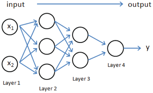
FIGURE 2-4: An example of the architecture of a neural network.
The figure shows a simple neural architecture. Note how the layers filter information in a progressive way. This is a feed-forward input because data feeds in one direction, forward, into the network. Only Layer 1 receives input from the original dataset; the other layers feed each other. Connections exclusively link the units in one layer with the units in the following layer (information flow from left to right). No connections exist between units in the same layer or with units outside the next layer. Moreover, the information pushes forward (from the left to the right). Processed data never returns to previous neuron layers.
Using a neural network is like using a stratified filtering system for water: You pour the water from above and the water is filtered at the bottom. The water has no way to go back; it just goes forward and straight down, and never laterally. In the same way, neural networks force data features to flow through the network and mix with each other only according to the network’s architecture. By using the best architecture to mix features, the neural network creates new composed features at every layer and helps achieve better predictions. Unfortunately, you have no way to determine the best architecture without empirically trying different solutions and testing whether the output data helps predict your target values after flowing through the network.
The first and last layers play an important role. The first layer, called the input layer, picks ups the features from each data example processed by the network. The last layer, called the output layer, releases the results.
A neural network can process only numeric, continuous information; it can’t be constrained to work with qualitative variables (for example, labels indicating a quality such as red, blue, or green in an image). You can process qualitative variables by transforming them into a continuous numeric value, such as a series of binary values. When a neural network processes a binary variable, the neuron treats the variable as a generic number and turns the binary values into other values, even negative ones, by processing across units.
Note the limitation of dealing only with numeric values because you can’t expect the last layer to output a nonnumeric label prediction. When dealing with a regression problem, the last layer is a single unit. Likewise, when you’re working with a classification and you have output that must choose from a number n of classes, unless you have a binary problem in which you predict only two classes, you should have n terminal units, each one representing a score linked to the probability of the represented class. However, when you have a binary classification problem, you can use a single output neuron, as in a regression problem, because you just predict the probability of a class and automatically infer the probability of the other class (because it is 100 percent minus the predicted probability).
To put the need for multiple input and terminal units into perspective, when classifying a multiclass problem such as an iris species, think about the famous Iris classification example, created by R. A. Fisher (https://archive.ics.uci.edu/ml/datasets/iris). In this case, the input layer has enough units for each of the attributes:
- Sepal length in cm
- Sepal width in cm
- Petal length in cm
- Petal width in cm
The output layer has as many units as species. In a neural network based on the Iris dataset, you therefore have three units representing one of the three Iris species:
- Setosa
- Versicolor
- Virginica
The predicted class is the one that gets the higher score at the end based on four input attributes.
 Some neural networks have special final layers, collectively called softmax, which can adjust the probability of each class based on the values received from a previous layer. In classification, the final layer may represent both a partition of probabilities thanks to softmax (a multiclass problem in which total probabilities sum to 100 percent) or an independent score prediction (because an example can have more classes, which is a multilabel problem in which summed probabilities can be more than 100 percent). When the classification problem is a binary classification, a single output suffices. Also, in regression, you can have multiple output units, each one representing a different regression problem. (For instance, in forecasting, you can have different predictions for the next day, week, month, and so on.)
Defining hidden layers
Neural networks have different layers, each one having its own weights and using its own activation function. Because the neural network segregates computations by layers, knowing the reference layer is important because you can account for certain units and connections. You can refer to every layer using a specific number and generically talk about each layer using the letter l.
Each layer can have a different number of units, and the number of units located between two layers dictates the number of connections. By multiplying the number of units in the starting layer with the number in the following layer, you can determine the total number of connections between the two: number of connections(l) = units(l) * units(l+1).
A matrix of weights, usually named with the uppercase Greek letter Theta (Θ), represents the connections. For ease of reading, the book uses the capital letter W, which is a fine choice because it is a matrix or a multidimensional array. Thus, you can use W1 to refer to the connection weights from layer 1 to layer 2, W2 for the connections from layer 2 to layer 3, and so on.
Weights represent the strength of the connection between neurons in the network. When the weight of the connection between two layers is small, it means that the network dumps values flowing between them and signals that taking this route won’t likely influence the final prediction. Alternatively, a large positive or negative value affects the values that the next layer receives, thus changing certain predictions. This approach is analogous to brain cells, which don’t stand alone but connect with other cells. As a person grows in experience, connections between neurons tend to weaken or strengthen to activate or deactivate certain brain network cell regions, causing other processing or an activity (a reaction to a danger, for instance, if the processed information signals a life-threatening situation).
Executing operations
Now that you know some conventions regarding layers, units, and connections, you can start examining the operations that neural networks execute in detail. To begin, you can call inputs and outputs in different ways:
- a: The result stored in a unit in the neural network after being processed by the activation function (called g). This is the final output that is sent further along the network.
- z: The multiplication between a and the weights from the W matrix. z represents the signal going through the connections, analogous to water in pipes that flows at a higher or lower pressure depending on the pipe diameter. In the same way, the values received from the previous layer become higher or lower because of the connection weights used to transmit them.
Each successive layer of units in a neural network progressively processes the values taken from the features. (Picture a conveyor belt.) As data transmits in the network, it arrives at each unit as a value produced by the summation of the values present in the previous layer and weighted by connections represented in the matrix W. When the data with added bias exceeds a certain threshold, the activation function increases the value stored in the unit; otherwise, it extinguishes the signal by reducing it. After processing by the activation function, the result is ready to push forward to the connection linked to the next layer. These steps repeat for each layer until the values reach the end and you have a result, as shown in Figure 2-5.

FIGURE 2-5: A detail of the feed-forward process in a neural network.
The figure shows a detail of the process that involves two units pushing their results to another unit. This series of events happens in every part of the network:
- The input A1 is multiplied by its weighting factor W1.
- The input A2 is multiplied by its weighting factor W2.
- The two weighted inputs are summed with a bias to produce the value z.
- The output, A3, is produced by the activation function, g, accepting the summed and biased value z. This output now goes to the next layer or is used as an output.
Considering the details of data movement through the neural network
When you understand the passage from two neurons to one, you can understand the entire feed-forward process, even when more layers and neurons are involved. For more explanation, here are the seven steps used to produce a prediction in a neural network made of four layers (refer to Figure 2-4):
- The first layer (notice the superscript 1 on a) loads the value of each feature in a different unit:
a(1)= X - The weights of the connections bridging the input layer with the second layer are multiplied by the values of the units in the first layer. A matrix multiplication weights and sums the inputs for the second layer together.
z(2)=W(1)a(1) - The algorithm adds a bias constant to layer two before running the activation function. The activation function transforms the second layer inputs. The resulting values are ready to pass to the connections.
a(2) = g(z(2) + bias(2)) - The third layer connections weight and sum the outputs of layer two.
z(3) = W(2)a(2) - The algorithm adds a bias constant to layer three before running the activation function. The activation function transforms the layer-three inputs.
a(3) = g(z(3) + bias(3)) - The layer-three outputs are weighted and summed by the connections to the output layer.
z(4) = W(3)a(3) - Finally, the algorithm adds a bias constant to layer four before running the activation function. The output units receive their inputs and transform the input using the activation function. After this final transformation, the output units are ready to release the resulting predictions of the neural network.
a(4) = g(z(4) + bias(4))
The activation function plays the role of a signal filter, helping to select the relevant signals and avoid the weak and noisy ones (because it discards values below a certain threshold). Activation functions also provide nonlinearity to the output because they enhance or damp the values passing through them in a nonproportional way.
The weights of the connections provide a way to mix and compose the features in a new way, creating new features in a way not too different from a polynomial expansion. The activation renders nonlinear the resulting recombination of the features by the connections. Both of these neural network components enable the algorithm to learn complex target functions that represent the relationship between the input features and the target outcome.
Using backpropagation to adjust learning
From an architectural perspective, a neural network does a great job of mixing signals from examples and turning them into new features to achieve an approximation of complex nonlinear functions (functions that you can’t represent as a straight line in the features’ space). To create this capability, neural networks work as universal approximators (for more details, go to https://www.techleer.com/articles/449-the-universal-approximation-theorem-for-neural-networks/), which means that they can guess any target function. However, you have to consider that one aspect of this feature is the capacity to model complex functions (representation capability), and another aspect is the capability to learn from data effectively.
Learning occurs in a brain because of the formation and modification of synapses between neurons, based on stimuli received by trial-and-error experience. Neural networks provide a way to replicate this process as a mathematical formulation called backpropagation. The following sections tell you more about backpropagation.
Delving into backpropagation beginnings
Since its early appearance in the 1970s, the backpropagation algorithm has been given many fixes. Each neural network learning process improvement resulted in new applications and a renewed interest in the technique. In addition, the current deep learning revolution, a revival of neural networks, which were abandoned at the beginning of the 1990s, is the result of key advances in the way neural networks learn from their errors. As seen in other algorithms, the cost function activates the necessity to learn certain examples better (large errors correspond to high costs). When an example with a large error occurs, the cost function outputs a high value that is minimized by changing the parameters in the algorithm. The optimization algorithm determines the best action for reducing the high outputs from the cost function.
In linear regression, finding an update rule to apply to each parameter (the vector of beta coefficients) is straightforward. However, in a neural network, things are a bit more complicated. The architecture is variable and the parameter coefficients (the connections) relate to each other because the connections in a layer depend on how the connections in the previous layers recombined the inputs. The solution to this problem is the backpropagation algorithm. Backpropagation is a smart way to propagate the errors back into the network and make each connection adjust its weights accordingly. If you initially feed-forward propagated information to the network, it’s time to go backward and give feedback on what went wrong in the forward phase.
Backpropagation is how adjustments required by the optimization algorithm are propagated through the neural network. Distinguishing between optimization and backpropagation is important. In fact, all neural networks use backpropagation, but the “Relying on a smart optimizer” section, later in this chapter, discusses many different optimization algorithms.
Understanding how backpropagation works
Discovering how backpropagation works isn’t complicated, even though demonstrating how it works using formulas and mathematics requires derivatives and the proving of some formulations, which is quite tricky and beyond the scope of this book. To get a sense of how backpropagation operates, start from the end of the network, just at the moment when an example has been processed and you have a prediction as an output. At this point, you can compare the prediction with the real result and, by subtracting the two values, get an offset, which is the error. Now that you know the mismatch of the results at the output layer, you can progress backward to distribute the error information to all the units in the network.
The cost function of a neural network for classification is based on cross-entropy (as seen in logistic regression):
Cost = y * log(hW(X)) + (1 - y)*log(1 - hW(X))
This is a formulation involving logarithms. It refers to the prediction produced by the neural network and expressed as hW(X) (which reads as the result of the network given connections W and X as input). To make things easier, when thinking of the cost, it helps to think of it as computing the offset between the expected results and the neural network output.
The first step in transmitting the error back into the network relies on backward multiplication. Because the values fed to the output layer are made of the contributions of all units, proportional to the weight of their connections, you can redistribute the error according to each contribution. For instance, the vector of errors of a layer n in the network, a vector indicated by the Greek letter delta (δ), is the result of the following formulation:
δ (n) = W(n)T * δ (n+1)
This formula says that, starting from the final delta, you can continue redistributing delta going backward in the network and using the weights you used to push forward the value to partition the error to the different units. In this way, you can get the terminal error redistributed to each neural unit, and you can use it to recalculate a more appropriate weight for each network connection to minimize the error. To update the weights W of layer l, you just apply the following formula:
W(l) = W(1) + η* δ (1) * g'(z(l)) *a(1)
The formula may appear puzzling at first sight, but it is a summation, and you can discover how it works by looking at its elements. First, look at the function g'. It's the first derivative of the activation function g, evaluated by the input values z. In fact, this is the Gradient Descent method. Gradient Descent determines how to reduce the error measure by finding, among the possible combinations of values, the weights that most reduce the error.
The Greek letter eta (η), sometimes also called alpha (α) or epsilon (ε) depending on the textbook you consult, is the learning rate. As found in other algorithms, it reduces the effect of the update suggested by the Gradient Descent derivative. In fact, the direction provided may be only partially correct or just roughly correct. By taking multiple small steps in the descent, the algorithm can take a more precise direction toward the global minimum error, which is the target you want to achieve (that is, a neural network producing the least possible prediction error).
Setting the eta value
Different methods are available for setting the right eta value, because the optimization largely depends on it. One method sets the eta value starting high and reduces it during the optimization process. Another method variably increases or decreases eta based on the improvements obtained by the algorithm: Large improvements call a larger eta (because the descent is easy and straight); smaller improvements call a smaller eta so that the optimization will move slower, looking for the best opportunities to descend. Think of it as being on a tortuous path in the mountains: You slow down and try not to be struck or thrown off the road as you descend.
Most implementations offer an automatic setting of the correct eta. You need to note this setting’s relevance when training a neural network because it’s one of the important parameters to tweak to obtain better predictions, together with the layer architecture. Weight updates can happen in different ways with respect to the training set of examples:
- Online mode: The weight update happens after every example traverses the network. In this way, the algorithm treats the learning examples as a stream from which to learn in real time. This mode is perfect when you have to learn out of core, that is, when the training set can’t fit into RAM memory. However, this method is sensitive to outliers, so you have to keep your learning rate low. (Consequently, the algorithm is slow to converge to a solution.)
- Batch mode: The weight update happens after processing all the examples in the training set. This technique makes optimization fast and less subject to having variance appear in the example stream. In batch mode, the backpropagation considers the summed gradients of all examples.
- Mini-batch (or stochastic) mode: The weight update happens after the network has processed a subsample of randomly selected training set examples. This approach mixes the advantages of online mode (low memory usage) and batch mode (a rapid convergence) while introducing a random element (the subsampling) to avoid having the Gradient Descent stuck in a local minima (a drop in value that isn’t the true minimum).
Understanding More about Neural Networks
You can find many discussions about neural network architectures online (such as the one at https://www.kdnuggets.com/2018/02/8-neural-network-architectures-machine-learning-researchers-need-learn.html). The problem, however, is that they all quickly become insanely complex, making normal people want to pull out their hair. Some unwritten law seems to say that math has to become instantly abstract and so complicated that no mere mortal can understand it, but anyone can understand a neural network. The material in the “Hitting Complexity with Neural Networks” section, earlier in this chapter, gives you a good start. Even though this earlier section does rely a little on math to get its point across, the math is relatively simple. The following sections help you use what you now know about neural networks to create an example using Python or R.
Getting an overview of the neural network process
What a neural network truly represents is a kind of filter. You pour data into the top, that data percolates through the various layers you create, and an output appears at the bottom. The things that differentiate neural networks are the same sorts of things you might look for in a filter. For example, the kind of algorithm you choose determines the kind of filtering the neural network will perform. You may want to filter the lead out of the water but leave the calcium and other beneficial minerals intact, which means choosing a kind of filter to do that.
However, filters can come with controls. For example, you might choose to filter particles of one size but let particles of another size pass. The use of weights and biases in a neural network are simply a kind of control. You adjust the control to fine-tune the filtering you receive. In this case, because you’re using electrical signals modeled after those found in the brain, a signal is allowed to pass when it meets a particular condition — a threshold defined by an activation function. To keep things simple for now, though, just think about it as you would adjustments to any filter’s basic operation.
You can monitor the activity of your filter. However, unless you want to stand there all day looking at it, you probably rely on some sort of automation to ensure that the filter’s output remains constant. This is where an optimizer comes into play. By optimizing the output of the neural network, you see the results you need without constantly tuning it manually.
Finally, you want to allow a filter to work at a speed and capacity that allows it to perform its tasks correctly. Pouring water or some other substance through the filter too quickly would cause it to overflow. If you don’t pour fast enough, the filter might clog or work erratically. Adjusting the learning rate of the optimizer of a neural network enables you to ensure that the neural network produces the output you want. It’s like adjusting the pouring rate of a filter.
Neural networks can seem hard to understand. The fact that much of what they do is shrouded in mathematical complexity doesn’t help matters. However, you don’t have to be a rocket scientist to understand what neural networks are all about. All you really need to do is break them down into manageable pieces and use the right perspective to look at them.
Defining the basic architecture
A neural network relies on numerous computation units, the neurons, arranged into hierarchical layers. Each neuron accepts inputs from all its predecessors and provides outputs to its successors until the neural network as a whole satisfies a requirement. At this point, the network processing ends and you receive the output.
All these computations occur singularly in a neural network. The network passes over each of them using loops for loop iterations. You can also leverage the fact that most of these operations are plain multiplications, followed by addition, and take advantage of the matrix calculations shown in Book 2, Chapter 3.
The example in this section creates a network with an input layer (whose dimensions are defined by the input), a hidden layer with three neurons, and a single output layer that tells whether the input is part of a class (a binary 0/1 answer). This architecture implies creating two sets of weights represented by two matrices (when you’re actually using matrices):
- The first matrix uses a size determined by the number of inputs x 3, represents the weights that multiply the inputs, and sums them into three neurons.
- The second matrix uses a size of 3 x 1, gathers all the outputs from the hidden layer, and makes that layer converge into the output.
Here’s the required Python script (which may take a while to complete running, depending on the speed of your system):
import numpy as np
from sklearn.datasets import make_moons
from sklearn.model_selection import train_test_split
import matplotlib.pyplot as plt
%matplotlib inline
def init(inp, out):
return np.random.randn(inp, out) / np.sqrt(inp)
def create_architecture(input_layer, first_layer,
output_layer, random_seed=0):
np.random.seed(random_seed)
layers = X.shape[1], 3 , 1
arch = list(zip(layers[:-1], layers[1:]))
weights = [init(inp, out) for inp, out in arch]
return weights
The interesting point of this initialization is that it uses a sequence of matrices to automate the network calculations. How the code initializes them matters because you can’t use numbers that are too small — there will be too little signal for the network to work. However, you must also avoid numbers that are too big because the calculations become too cumbersome to handle. Sometimes they fail, which causes the exploding gradient problem (wherein the neural network ceases to function because of the exploding values; see the article at https://machinelearningmastery.com/exploding-gradients-in-neural-networks/ for details) or, more often, causes saturation of the neurons, which means that you can’t correctly train a network because all the neurons are always activated.
Initializing your network using all zeros is always a bad idea because if all the neurons have the same value, they will react in the same way to the training input. No matter how many neurons the architecture contains, they operate as a single neuron.
The simpler solution is to start with initial random weights that are in the range required for the activation functions, which are the transformation functions that add flexibility to solving problems using the network. A possible simple solution is to set the weights to zero mean and one standard deviation, which in statistics is called the standard normal distribution and in the code appears as the np.random.radn command.
However, smarter weight initializations exist for more complex networks, such as those found in this article: https://towardsdatascience.com/weight-initialization-techniques-in-neural-networks-26c649eb3b78.
Moreover, because each neuron accepts the inputs of all previous neurons, the code rescales the random normal distributed weights using the square root of the number of inputs. Consequently, the neurons and their activation functions always compute the right size for everything to work smoothly.
Documenting the essential modules
The architecture is just one part of a neural network. You can imagine it as the structure of the network. Architecture explains how the network processes data and provides results. However, for any processing to happen, you also need to code the neural network's core functionalities.
The first building block of the network is the activation function. The “Considering the neuron” section, earlier in this chapter, details a few activation functions used in neural networks without explaining them in much detail. The example in this section provides code for the sigmoid function, one of the basic neural network activation functions. The sigmoid function is a step up from the Heaviside step function, which acts as a switch that activates at a certain threshold. A Heaviside step function outputs 1 for inputs above the threshold and 0 for inputs below it.
The sigmoid functions outputs 0 or 1, respectively, for small input values below zero or high values above zero. For input values in the range between –5 and +5, the function outputs values in the range 0–1, slowly increasing the output of released values until it reaches around 0.2 and then growing fast in a linear way until reaching 0.8. It then decreases again as the output rate approaches 1. Such behavior represents a logistic curve, which is useful for describing many natural phenomena, such as the growth of a population that starts growing slowly and then fully blossoms and develops until it slows down before hitting a resource limit (such as available living space or food).
In neural networks, the sigmoid function is particularly useful for modeling inputs that resemble probabilities, and it’s differentiable, which is a mathematical aspect that helps reverse its effects and works out the best backpropagation phase:
def sigmoid(z):
return 1/(1 + np.exp(-z))
def sigmoid_prime(s):
return s * (1 -s)
After you have an activation function, you can create a forward procedure, which is a matrix multiplication between the input to each layer and the weights of the connection. After completing the multiplication, the code applies the activation function to the results to transform them in a nonlinear way. The following code embeds the sigmoid function into the network’s feed-forward code. Of course, you can use any other activation function if desired:
def feed_forward(X, weights):
a = X.copy()
out = list()
for W in weights:
z = np.dot(a, W)
a = sigmoid(z)
out.append(a)
return out
By applying the feed forward to the complete network, you finally arrive at a result in the output layer. Now you can compare the output against the real values you want the network to obtain. The accuracy function determines whether the neural network is performing predictions well by comparing the number of correct guesses to the total number of predictions provided:
def accuracy(true_label, predicted):
correct_preds = np.ravel(predicted)==true_label
return np.sum(correct_preds) / len(true_label)
The backpropagation function comes next because the network is working but all or some of the predictions are incorrect. Correcting predictions during training enables you to create a neural network that can take on new examples and provide good predictions. The training is incorporated into its connection weights as patterns present in data that can help predict the results correctly.
To perform backpropagation, you first compute the error at the end of each layer (this architecture has two). Using this error, you multiply it by the derivative of the activation function. The result provides you with a gradient, that is, the change in weights necessary to compute predictions more correctly. The code starts by comparing the output with the correct answers (l2_error), and then computes the gradients, which are the necessary weight corrections (l2_delta). The code then proceeds to multiply the gradients by the weights the code must correct. The operation distributes the error from the output layer to the intermediate one (l1_error). A new gradient computation (l1_delta) also provides the weight corrections to apply to the input layer, which completes the process for a network with an input layer, a hidden layer, and an output layer:
def backpropagation(l1, l2, weights, y):
l2_error = y.reshape(-1, 1) - l2
l2_delta = l2_error * sigmoid_prime(l2)
l1_error = l2_delta.dot(weights[1].T)
l1_delta = l1_error * sigmoid_prime(l1)
return l2_error, l1_delta, l2_delta
This is a Python code translation, in simplified form, of the formulas you find in the “Understanding how backpropagation works” section, earlier in this chapter. The cost function is the difference between the network's output and the correct answers. The example doesn’t add biases during the feed-forward phase, which reduces the complexity of the backpropagation process and makes it easier to understand.
After backpropagation assigns each connection its part of the correction that should be applied over the entire network, you adjust the initial weights to represent an updated neural network. You do so by adding to the weights of each layer, the multiplication of the input to that layer, and the delta corrections for the layer as a whole. This is a Gradient Descent method step in which you approach the solution by taking repeated small steps in the right direction, so you may need to adjust the step size used to solve the problem. The alpha parameters help make changing the step size possible. Using a value of 1 won’t affect the impact of the previous weight correction, but values smaller than 1 effectively reduce it:
def update_weights(X, l1, l1_delta, l2_delta, weights,
alpha=1.0):
weights[1] = weights[1] + (alpha * l1.T.dot(l2_delta))
weights[0] = weights[0] + (alpha * X.T.dot(l1_delta))
return weights
A neural network is not complete if it can only learn from data, but not predict. The last predict function pushes new data using feed forward, reads the last output layer, and transforms its values to problem predictions. Because the sigmoid activation function is so adept at modeling probability, the code uses a value halfway between 0 and 1, that is, 0.5, as the threshold for having a positive or negative output. Such a binary output could help in classifying two classes or a single class against all the others if a dataset has three or more types of outcomes to classify.
def predict(X, weights):
_, l2 = feed_forward(X, weights)
preds = np.ravel((l2 > 0.5).astype(int))
return preds
At this point, the example has all the parts that make a neural network work. You just need a problem that demonstrates how the neural network works.
Solving a simple problem
In this section, you test the neural network code you wrote by asking it to solve a simple, but not banal, data problem. The code uses the Scikit-learn package’s make_moons function to create two interleaving circles of points shaped as two half moons. Separating these two circles requires an algorithm capable of defining a nonlinear separation function that generalizes to new cases of the same kind. A neural network, such as the one presented earlier in the chapter, can easily handle the challenge.
np.random.seed(0)
coord, cl = make_moons(300, noise=0.05)
X, Xt, y, yt = train_test_split(coord, cl,
test_size=0.30,
random_state=0)
plt.scatter(X[:,0], X[:,1], s=25, c=y, cmap=plt.cm.Set1)
plt.show()
The code first sets the random seed to produce the same result anytime you want to run the example. The next step is to produce 300 data examples and split them into a train and a test dataset. (The test dataset is 30 percent of the total.) The data consists of two variables representing the x and y coordinates of points on a Cartesian graph. Figure 2-6 shows the output of this process.

FIGURE 2-6: Two interleaving moon-shaped clouds of data points.
Because learning in a neural network happens in successive iterations (called epochs), after creating and initializing the sets of weights, the code loops 30,000 iterations of the two half moons data (each passage is an epoch). On each iteration, the script calls some of the previously prepared core neural network functions:
- Feed forward the data through the entire network.
- Backpropagate the error back into the network.
- Update the weights of each layer in the network, based on the backpropagated error.
- Compute the training and validation errors.
The following code uses comments to detail when each function operates:
weights = create_architecture(X, 3, 1)
for j in range(30000 + 1):
# First, feed forward through the hidden layer
l1, l2 = feed_forward(X, weights)
# Then, error backpropagation from output to input
l2_error, l1_delta, l2_delta = backpropagation(l1,
l2, weights, y)
# Finally, updating the weights of the network
weights = update_weights(X, l1, l1_delta, l2_delta,
weights, alpha=0.05)
# From time to time, reporting the results
if (j % 5000) == 0:
train_error = np.mean(np.abs(l2_error))
print('Epoch {:5}'.format(j), end=' - ')
print('error: {:0.4f}'.format(train_error),
end= ' - ')
train_accuracy = accuracy(true_label=y,
predicted=(l2 > 0.5))
test_preds = predict(Xt, weights)
test_accuracy = accuracy(true_label=yt,
predicted=test_preds)
print('acc: train {:0.3f}'.format(train_accuracy),
end= '/')
print('test {:0.3f}'.format(test_accuracy))
Variable j counts the iterations. At each iteration, the code tries to divide j by 5,000 and check whether the division leaves a module. When the module is zero, the code infers that 5,000 epochs have passed since the previous check, and summarizing the neural network error is possible by examining its accuracy (how many times the prediction is correct with respect to the total number of predictions) on the training set and on the test set. The accuracy on the training set shows how well the neural network is fitting the data by adapting its parameters by the backpropagation process. The accuracy on the test set provides an idea of how well the solution generalized to new data and thus whether you can reuse it.
The test accuracy should matter the most because it shows the potential usability of the neural network with other data. The training accuracy just tells you how the network scores with the present data you are using. Here is an example of what you might see as output:
Epoch 0 - error: 0.5077 - acc: train 0.462/test 0.656
Epoch 5000 - error: 0.0991 - acc: train 0.952/test 0.944
Epoch 10000 - error: 0.0872 - acc: train 0.952/test 0.944
Epoch 15000 - error: 0.0809 - acc: train 0.957/test 0.956
Epoch 20000 - error: 0.0766 - acc: train 0.967/test 0.956
Epoch 25000 - error: 0.0797 - acc: train 0.962/test 0.967
Epoch 30000 - error: 0.0713 - acc: train 0.957/test 0.956
Looking Under the Hood of Neural Networks
After you know how neural networks basically work, you need a better understanding of what differentiates them. Beyond the different architectures, the choice of the activation functions, the optimizers and the neural network's learning rate can make the difference. Knowing basic operations isn’t enough because you won’t get the results you want. Looking under the hood helps you understand how you can tune your neural network solution to model specific problems. In addition, understanding the various algorithms used to create a neural network will help you obtain better results with less effort and in a shorter time. The following sections focus on three areas of neural network differentiation.
Choosing the right activation function
An activation function simply defines when a neuron fires. Consider it a sort of tipping point: Input of a certain value won’t cause the neuron to fire because it’s not enough, but just a little more input can cause the neuron to fire. A neuron is defined in a simple manner, as follows:
y = ∑ (weight * input) + bias
The output, y, can be any value between + infinity and – infinity. The problem, then, is to decide on what value of y is the firing value, which is where an activation function comes into play. The activation function determines which value is high or low enough to reflect a decision point in the neural network for a particular neuron or group of neurons.
As with everything else in neural networks, you don't have just one activation function. You use the activation function that works best in a particular scenario. With this in mind, you can break the activation functions into these categories:
- Step: A step function (also called a binary function) relies on a specific threshold for making the decision about activating or not. Using a step function means that you know which specific value will cause an activation. However, step functions are limited in that they’re either fully activated or fully deactivated — no shades of gray exist. Consequently, when attempting to determine which class is most likely correct based on a given input, a step function won’t work.
- Linear: A linear function (
A = cx) provides a straight-line determination of activation based on input. Using a linear function helps you determine which output to activate based on which output is most correct (as expressed by weighting). However, linear functions work only as a single layer. If you were to stack multiple linear function layers, the output would be the same as using a single layer, which defeats the purpose of using neural networks. Consequently, a linear function may appear as a single layer, but never as multiple layers. - Sigmoid: A sigmoid function (
A = 1 / 1 + e-x), which produces a curve shaped like the letter C or S, is nonlinear. It begins by looking sort of like the step function, except that the values between two points actually exist on a curve, which means that you can stack sigmoid functions to perform classification with multiple outputs. The range of a sigmoid function is between 0 and 1, not – infinity to + infinity as with a linear function, so the activations are bound within a specific range. However, the sigmoid function suffers from a problem called vanishing gradient, which means that the function refuses to learn after a certain point because the propagated error shrinks to zero as it approaches faraway layers. - TanH: A tanh function (
A = (2 / 1 + e-2x) – 1) is actually a scaled sigmoid function. It has a range of –1 to 1, so again, it's a precise method for activating neurons. The big difference between sigmoid functions and tanh functions is that the tanh function gradient is stronger, which means that detecting small differences is easier, making classification more sensitive. Like the sigmoid function, tanh suffers from vanishing gradient issues. - ReLU: A ReLU function (
A(x) = max(0, x)) provides an output in the range of 0 to infinity, so it’s similar to the linear function except that it’s also nonlinear, enabling you to stack ReLU functions. An advantage of ReLU is that it requires less processing power because fewer neurons fire. The lack of activity as the neuron approaches the 0 part of the line means that there are fewer potential outputs to look at. However, this advantage can also become a disadvantage when you have a problem called the dying ReLU. After a while, the neural network weights don’t provide the desired effect any longer (the network simply stops learning) and the affected neurons die — meaning that they don’t respond to any input.
Also, the ReLU has some variants that you should consider:
- ELU (Exponential Linear Unit): Differs from ReLU when the inputs are negative. In this case, the outputs don’t go to zero but instead slowly decrease to –1 exponentially.
- PReLU (Parametric Rectified Linear Unit): Differs from ReLU when the inputs are negative. In this case, the output is a linear function whose parameters are learned using the same technique as any other parameter of the network.
- LeakyReLU: Similar to PReLU but the parameter for the linear side is fixed.
Relying on a smart optimizer
An optimizer serves to ensure that your neural network performs fast and correctly models whatever problem you want to solve by modifying the neural network’s biases and weights. It turns out that an algorithm performs this task, but you must choose the correct algorithm to obtain the results you expect. As with all neural network scenarios, you have a number of optional algorithm types from which to choose (see https://keras.io/optimizers/):
- Stochastic Gradient Descent (SGD)
- RMSProp
- AdaGrad
- AdaDelta
- AMSGrad
- Adam and its variants, Adamax and Nadam
An optimizer works by minimizing or maximizing the output of an objective function (also known as an error function) represented as E(x). This function is dependent on the model’s internal learnable parameters used to calculate the target values (Y) from the predictors (X). Two internal learnable parameters are weights (W) and bias (b). The various algorithms have different methods of dealing with the objective function.
You can categorize the optimizer functions by the manner in which they deal with the derivative (dy/dx), which is the instantaneous change of y with respect to x. Here are the two levels of derivative handling:
- First order: These algorithms minimize or maximize the objective function using gradient values with respect to the parameters.
- Second order: These algorithms minimize or maximize the object function using the second-order derivative values with respect to the parameters. The second-order derivative can give a hint as to whether the first-order derivative is increasing or decreasing, which provides information about the curvature of the line.
You commonly use first-order optimization techniques, such as Gradient Descent, because they require fewer computations and tend to converge to a good solution relatively fast when working on large datasets.
Setting a working learning rate
Each optimizer has completely different parameters to tune. One constant is fixing the learning rate, which represents the rate at which the code updates the network’s weights (such as the alpha parameter used in the example for this chapter). The learning rate can affect both the time the neural network takes to learn a good solution (the number of epochs) and the result. In fact, if the learning rate is too low, your network will take forever to learn. Setting the value too high causes instability when updating the weights, and the network won't ever converge to a good solution.
Choosing a learning rate that works is daunting because you can effectively try values in the range from 0.000001 to 100. The best value varies from optimizer to optimizer. The value you choose depends on what type of data you have. Theory can be of little help here; you have to test different combinations before finding the most suitable learning rate for training your neural network successfully.
In spite of all the math surrounding neural networks, tuning them and having them work best is mostly a matter of empirical efforts in trying different combinations of architectures and parameters.
Explaining Deep Learning Differences with Other Forms of AI
Given the embarrassment of riches that pertain to AI as a whole, such as large amounts of data, new and powerful computational hardware available to everyone, and plenty of private and public investments, you may be skeptical about the technology behind deep learning, which consists of neural networks that have more neurons and hidden layers than in the past. Deep networks contrast with the simpler, shallower networks of the past, which featured one or two hidden layers at best. Many solutions that render the deep learning of today possible are not at all new, but deep learning uses them in new ways.
Deep learning isn't simply a rebranding of an old technology, the perceptron (see the section “Understanding perceptron functionality,” earlier in this chapter). Deep learning works better because of the sophistication it adds through the full use of powerful computers and the availability of better (not just more) data. Deep learning also implies a profound qualitative change in the capabilities offered by the technology along with new and astonishing applications. The presence of these capabilities modernizes old but good neural networks, transforming them into something new. The following sections describe just how deep learning achieves its task.
Adding more layers
You may wonder why deep learning has blossomed only now when the technology used as the foundation of deep learning existed long ago. Computers are more powerful today, and deep learning can access huge amounts of data. However, these answers point only to important problems with deep learning in the past, and lower computing power along with less data weren’t the only insurmountable obstacles. Until recently, deep learning also suffered from a key technical problem that kept neural networks from having enough layers to perform truly complex tasks.
Because it can use many layers, deep learning can solve problems that are out of reach of machine learning, such as image recognition, machine translation, and speech recognition. When fitted with only a few layers, a neural network is a perfect universal function approximator, which is a system that can re-create any possible mathematical function. When fitted with many more layers, a neural network becomes capable of creating, inside its internal chain of matrix multiplications, a sophisticated system of representations to solve complex problems. To understand how a complex task like image recognition works, consider this process:
- A deep learning system trained to recognize images (such as a network capable of distinguishing photos of dogs from those featuring cats) defines internal weights that have the capability to recognize a picture topic.
- After detecting each single contour and corner in the image, the deep learning network assembles all such basic traits into composite characteristic features.
- The network matches such features to an ideal representation that provides the answer.
In other words, a deep learning network can distinguish dogs from cats using its internal weights to define a representation of what, ideally, a dog and a cat should resemble. It then uses these internal weights to match any new image you provide it with.
One of the earliest achievements of deep learning that made the public aware of its potentiality is the cat neuron. The Google Brain team, run at that time by Andrew Ng and Jeff Dean, put together 16,000 computers to calculate a deep learning network with more than a billion weights, thus enabling unsupervised learning from YouTube videos. The computer network could even determine by itself, without any human intervention, what a cat is, and Google scientists managed to dig out of the network a representation of how the network itself expected a cat should look (see the “Wired” article at https://www.wired.com/2012/06/google-x-neural-network/).
During the time that scientists couldn’t stack more layers into a neural network because of the limits of computer hardware, the potential of the technology remained buried, and scientists ignored neural networks. The lack of success added to the profound skepticism that arose around the technology during the last AI winter (1987 to 1993). However, what really prevented scientists from creating something more sophisticated was the problem with vanishing gradients.
A vanishing gradient occurs when you try to transmit a signal through a neural network and the signal quickly fades to near zero values; it can’t get through the activation functions. This happens because neural networks are chained multiplications. Each below-zero multiplication decreases the incoming values rapidly, and activation functions need large enough values to let the signal pass. The farther neuron layers are from the output, the higher the likelihood that they’ll get locked out of updates because the signals are too small and the activation functions will stop them. Consequently, your network stops learning as a whole, or it learns at an incredibly slow pace.
Every attempt at putting together and testing complex networks ended in failure during the last AI winter because the backpropagation algorithm couldn’t update the layers nearer the input, thus rendering any learning from complex data, even when such data was available at the time, almost impossible. Today, deep networks are possible thanks to the studies of scholars from the University of Toronto in Canada, such as Geoffrey Hinton (https://www.utoronto.ca/news/artificial-intelligence-u-t), who insisted on working on neural networks even when they seemed to most to be an old-fashioned machine learning approach.
Professor Hinton, a veteran of the field of neural networks (he contributed to defining the backpropagation algorithm), and his team in Toronto devised a few methods to circumvent the problem of vanishing gradients. He opened the field to rethinking new solutions that made neural networks a crucial tool in machine learning and AI again.
Professor Hinton and his team are memorable also for being among the first to test GPU usage in order to accelerate the training of a deep neural network. In 2012, they won an open competition, organized by the pharmaceutical company Merck and by Kaggle (https://www.kaggle.com/, a website for data science competitions), using their most recent deep learning discoveries. This event brought great attention to the Hinton team’s work. You can read all the details of the Hinton team’s revolutionary achievement with neural network layers from this Geoffrey Hinton interview: http://blog.kaggle.com/2012/11/01/deep-learning-how-i-did-it-merck-1st-place-interview/.
Changing the activations
Geoffrey Hinton’s team (see preceding section) was able to add more layers to a neural architecture because of two solutions that prevented trouble with backpropagation:
-
They prevented the exploding gradients problem by using smarter network initialization. An exploding gradient differs from a vanishing gradient in that it can make a network blow up (stop functioning because of extremely high values) as the exploding gradient becomes too large to handle.
Your network can explode unless you correctly initialize the network to prevent it from computing large weight numbers. Then you solve the problem of vanishing gradients by changing the network activations. - The team realized that passing a signal through various activation layers tended to damp the backpropagation signal until it became too faint to pass anymore after examining how a sigmoid activation worked. They used a new activation as the solution for this problem. The choice of which algorithm to use fell to an old activation type of ReLU. An ReLU activation stopped the received signal if it was below zero, assuring the nonlinearity characteristic of neural networks and letting the signal pass as it was if above zero. (Using this type of activation is an example of combining old but still good technology with current technology.) Figure 2-7 shows how this process works.

FIGURE 2-7: How the ReLU activation function works in receiving and releasing signals.
The ReLU worked incredibly well and let the backpropagation signal arrive at the initial deep network layers. When the signal is positive, its derivative is 1. You can also find proof of the ReLU derivative in looking at Figure 2-7. Note that the rate of change is constant and equivalent to a unit when the input signal is positive (whereas when the signal is negative, the derivative is 0, thus preventing the signal from passing).
You can calculate the ReLU function using f(x)=max(0,x). The use of this algorithm increased training speed a lot, allowing fast training of even deeper networks without incurring any dead neurons. A dead neuron is one that the network can't activate because the signals are too faint.
Adding regularization by dropout
The other introduction to deep learning made by Hinton’s team (see preceding sections in this chapter) to complete the initial deep learning solution aimed at regularizing the network. A regularized network limits the network weights, which keeps the network from memorizing the input data and generalizing the witnessed data patterns.
Previous discussions in this chapter (see especially the “Adding more layers” section) note that certain neurons memorize specific information and force the other neurons to rely on this stronger neuron, causing the weak neurons to give up learning anything useful themselves (a situation called co-adaptation). To prevent co-adaptation, the code temporary switches off the activation of a random portion of neurons in the network.
As you see from the left side of Figure 2-8, the weights normally operate by multiplying their inputs into outputs for the activations. To switch off activation, the code multiplies a mask made of a random mix of ones and zeros with the results. If the neuron is multiplied by one, the network passes its signal. When a neuron is multiplied by zero, the network stops its signal, forcing other neurons not to rely on it in the process.
Dropout works only during training and doesn’t touch any part of the weights. It simply masks and hides part of the network, forcing the unmasked part to take a more active role in learning data patterns. During prediction time, dropout doesn’t operate, and the weights are numerically rescaled to account for the fact that they didn’t work together during training.

FIGURE 2-8: Dropout temporarily rules out 40 percent of neurons from the training.
Using online learning
Neural networks are more flexible than other machine learning algorithms, and they can continue to train as they work on producing predictions and classifications. This capability comes from optimization algorithms that allow neural networks to learn, which can work repeatedly on small samples of examples (called batch learning) or even on single examples (called online learning). Deep learning networks can build their knowledge step by step and remain receptive to new information that may arrive (in a manner similar to a baby’s mind, which is always open to new stimuli and to learning experiences).
For instance, a deep learning application on a social media website can train on cat images. As people post photos of cats, the application recognizes them and tags them with an appropriate label. When people start posting photos of dogs on the social network, the neural network doesn’t need to restart training; it can continue by learning images of dogs as well. This capability is particularly useful for coping with the variability of Internet data. A deep learning network can be open to novelty and adapt its weights to deal with it.
Transferring learning
Flexibility is handy even when a network completes its training, but you must reuse it for purposes different from the initial learning. Networks that distinguish objects and correctly classify them require a long time and a lot of computational capacity to learn what to do. Extending a network’s capability to new kinds of images that weren’t part of the previous learning means transferring the knowledge to this new problem (transfer learning).
For instance, you can transfer a network that’s capable of distinguishing between dogs and cats to perform a job that involves spotting dishes of macaroni and cheese. You use the majority of the layers of the network as they are (you freeze them) and then work on the final, output layers (fine-tuning). In a short time, and with fewer examples, the network will apply what it learned in distinguishing dogs and cats to macaroni and cheese. It will perform even better than a neural network trained only to recognize macaroni and cheese.
Transfer learning is something new to most machine learning algorithms and opens a possible market for transferring knowledge from one application to another, from one company to another. Google is already doing that, actually sharing its immense data repository by making public the networks that it built on it (as detailed in this post: https://techcrunch.com/2017/06/16/object-detection-api/). This is a step in democratizing deep learning by allowing everyone to access its potentiality.
Learning end to end
Finally, deep learning allows end-to-end learning, which means that it solves problems in an easier and more straightforward way than previous deep learning solutions. This flexibility might result in a greater impact when solving problems.
You may want to solve a difficult problem, such as having the AI recognize known faces or drive a car. When using the classical AI approach, you had to split the problem into more manageable subproblems to achieve an acceptable result in a feasible time. For instance, if you wanted to recognize faces in a photo, previous AI systems arranged the problem into parts, as follows:
- Find the faces in the photo.
- Crop the faces from the photo.
- Process the cropped faces to have a pose similar to an ID card photo.
- Feed the processed cropped faces as learning examples to a neural network for image recognition.
Today, you can feed the photo to a deep learning architecture, guide it to learn to find faces in the images, and then use the deep learning architecture to classify them. You can use the same approach for language translation, speech recognition, or even self-driving cars. In all cases, you simply pass the input to a deep learning system and obtain the wanted result.