
Chapter 3
Working with Scalars, Vectors, and Matrices
IN THIS CHAPTER
![]() Using matrixes and vectors to perform calculations
Using matrixes and vectors to perform calculations
![]() Obtaining the correct combinations
Obtaining the correct combinations
![]() Employing recursive techniques to obtain specific results
Employing recursive techniques to obtain specific results
![]() Considering ways to speed calculations
Considering ways to speed calculations
In Book 2, Chapter 1, you discover techniques for locating the data you need and use it for data science needs (Book 2, Chapter 4 continues this discussion). Simply knowing how to control a language by using its constructs to perform tasks isn’t enough, though. The goal of mathematical algorithms is to turn one kind of data into another kind of data. Manipulating data means taking raw input and doing something with it to achieve a desired result. For example, until you do something with traffic data, you can’t see the patterns that emerge that tell you where to spend additional money in improvements. The traffic data in its raw form does nothing to inform you; you must manipulate it to see the pattern in a useful manner. Therefore, those arcane mathematical symbols are useful after all. You use them as a sort of machine to turn raw data into something helpful, which is what you discover in this chapter.
In times past, people actually had to perform the various manipulations to make data useful by hand, which required advanced knowledge of math. Fortunately, you can find Python and R libraries to perform most of these manipulations using a little code. (In fact, both languages provide a great deal of native capability in this regard, with R being superior in this instance.) You don’t have to memorize arcane manipulations anymore — just know which language features to use. That’s what this chapter helps you achieve. You discover the means to perform various kinds of data manipulations using easily accessed language libraries designed especially for the purpose.
The chapter begins with scalar, vector, and matrix manipulations (see Chapter 2 of this minibook for the functional version of some of these techniques). You also discover how to speed up the calculations so that you spend less time manipulating the data and more time doing something really interesting with it, such as discovering just how to keep quite so many traffic jams from occurring.
 You don’t have to type the source code for this chapter manually. In fact, using the downloadable source is a lot easier. The source code for this chapter appears in the
 DSPD_0203_Data_Forms.ipynb source code file for Python and the DSPD_R_0203_Data_Forms.ipynb source code file for R. See the Introduction for details on how to find these source files.
Considering the Data Forms
To perform useful data science analysis, you often need to work with larger amounts of data that comes in specific forms. These forms have odd-sounding names, but the names are quite important. The three terms you need to know for this chapter are as follows:
- Scalar: A single base data item. For example, the number 2 shown by itself is a scalar.
- Vector: A one-dimensional array (essentially a list) of data items. For example, an array containing the numbers 2, 3, 4, and 5 would be a vector. You access items in a vector using a zero-based index, a pointer to the item you want. The item at index 0 is the first item in the vector, which is 2 in this case.
- Matrix: A two-or-more-dimensional array (essentially a table) of data items. For example, an array containing the numbers 2, 3, 4, and 5 in the first row and 6, 7, 8, and 9 in the second row is a matrix. You access items in a matrix using a zero-based row-and-column index. The item at row 0, column 0 is the first item in the matrix, which is 2 in this case.
Both Python and R provide substantial native capability to work with scalars, vectors, and matrices, but you still have to do considerable work to perform some tasks. To reduce the amount of work you do, you can rely on code written by other people and found in libraries. The following sections describe how to use the NumPy library to perform various tasks on scalars, vectors, and matrixes in Python. The downloadable source provides the same techniques for R developers.
Defining Data Type through Scalars
Every data form in Python and R begins with a scalar — a single item of a particular type. Precisely how you define a scalar depends on how you want to view objects within your code and the definitions of scalars for your language. For example, R provides these native, simple data types:
- Character
- Numeric (real or decimal)
- Integer
- Logical
- Complex
In many respects, R views strings as vectors of characters; the scalar element is a character, not a string. The difference is important when thinking about how R works with scalars. R also provides a character vector, which is different from an R string. You can read about the difference at https://www.gastonsanchez.com/r4strings/chars.html.
Python provides these native, simple data types:
- Boolean
- Integer
- Float
- Complex
- String
Note that Python doesn't include a character data type because it works with strings, not with characters. Yes, you can create a string containing a single character and you can interact with individual characters in a string, but there isn’t an actual character type. To see this fact for yourself, try this code:
anA = chr(65)
print(type(anA))
The output will be <class 'str'>, rather than <class 'char'>, which is what most languages would provide. Consequently, a string is a scalar in Python but a vector in R. Keeping language differences in mind will help as you perform analysis on your data.
Most languages also support what you might term as semi-native data types. For example, Python supports a Fraction data type that you create by using code like this:
from fractions import Fraction
x = Fraction(2, 3)
print(x)
print(type(x))
The fact that you must import Fraction means that it's not available all the time, as something like complex or int is. The tip-off that this is not a built-in class is the class output of <class 'fractions.Fraction'>. However, you get Fraction with your Python installation, which means that it's actually a part of the language (hence, semi-native).
 External libraries that define additional scalar data types are available for most languages. Access to these additional scalar types is important in some cases. Python provides access to just one data type in any particular category. For example, if you need to create a variable that represents a number without a decimal portion, you use the integer data type. Using a generic designation like this is useful because it simplifies code and gives the developer a lot less to worry about. However, in scientific calculations, you often need better control over how data appears in memory, which means having more data types — something that
 numpy provides for you. For example, you might need to define a particular scalar as a short (a value that is 16 bits long). Using numpy, you could define it as myShort = np.short(15). You could define a variable of precisely the same size using the np.int16 function. You can discover more about the scalars provided by the NumPy library for Python at https://www.numpy.org/devdocs/reference/arrays.scalars.html. You also find that most languages provide means of extending the native types (see the articles at https://docs.python.org/3/extending/newtypes.html and http://greenteapress.com/thinkpython/thinkCSpy/html/app02.html for additional details).
Creating Organized Data with Vectors
A vector is essentially a list or array of scalars that are grouped together to allow access using a single name. The underlying type is a scalar of some sort, but vectors act as a means of organizing the individual scalars and making them easier to work with. The following sections describe working with vectors from an overview perspective.
Defining a vector
The NumPy library provides essential functionality for scientific computing in Python. To use numpy, you import it using the following:
import numpy as np
Now you can access numpy using the common two-letter abbreviation np.
Use the numpy functions to create a vector. Here are some examples to try:
myVect1 = np.array([1, 2, 3, 4])
print(myVect1)
myVect2 = np.arange(1, 10, 2)
print(myVect2)
The array() function creates a vector using explicit numbers, while the arange() function creates a vector by defining a range. When using arange(), the first input tells the starting point, the second the stopping point, and the third the step between each number. A fourth argument lets you define the data type for the vector. You can also create a vector with a specific data type. All you need to do is specify the data type like this:
myVect3 = np.array(np.int16([1, 2, 3, 4]))
print(myVect3)
print(type(myVect3))
print(type(myVect3[0]))
The output tells you the facts about this particular array, including that the vector type is different from the scalar type of the items it contains:
[1 2 3 4]
<class 'numpy.ndarray'>
<class 'numpy.int16'>
Creating vectors of a specific type
In some cases, you need special numpy functions to create a vector (or a matrix) of a specific type. For example, some math tasks require that you fill the vector with ones. In this case, you use the ones function like this:
myVect4 = np.ones(4, dtype=np.int16)
print(myVect4)
The output shows that you do have a vector filled with a series of ones:
[1 1 1 1]
You can also use a zeros() function to fill a vector with zeros.
Performing math on vectors
You can perform basic math functions on vectors as a whole, which makes this incredibly useful and less prone to errors that can occur when using programming constructs such as loops to perform the same task. For example, print(myVect1 + 1) produces an output of [2, 3, 4, 5] when working with standard Python integers. As you might expect, print(myVect1 - 1) produces an output of [0, 1, 2, 3]. You can even use vectors in more complex math scenarios, such as print(2 ** myVect1), where the output is [ 2, 4, 8, 16].
 When you want to use NumPy functions and techniques on a standard Python list, you need to perform a conversion. Consider the following code:
myVect5 = [1, 2, 3, 4]
print(type(myVect5[0]))
print(type((2 ** np.array(myVect5))[0]))
The output shows that the type changes during the transition:
<class 'int'>
<class 'numpy.int32'>
Performing logical and comparison tasks on vectors
As a final thought on scalar and vector operations, you can also perform both logical and comparison tasks. For example, the following code performs comparison operations on two arrays:
a = np.array([1, 2, 3, 4])
b = np.array([2, 2, 4, 4])
print(a == b)
print(a < b)
The output tells you about the relationships between the two arrays:
[False True False True]
[ True False True False]
Starting with two vectors, a and b, the code checks whether the individual elements in a equal those in b. In this case, a[0] doesn't equal b[0]. However, a[1] does equal b[1]. The output is a vector of type bool that contains true or false values based on the individual comparisons. Likewise, you can check for instances when a < b and produce another vector containing the truth-values in this instance.
Logical operations rely on special functions. You check the logical output of the Boolean operators AND, OR, XOR, and NOT. Here is an example of the logical functions:
a = np.array([True, False, True, False])
b = np.array([True, True, False, False])
print(np.logical_or(a, b))
print(np.logical_and(a, b))
print(np.logical_not(a))
print(np.logical_xor(a, b))
The output tells you about the logical relationship between the two vectors:
[ True True True False]
[ True False False False]
[False True False True]
[False True True False]
You can also use numeric input to these functions. When using numeric input, a 0 is false and a 1 is true. As with comparisons, the functions work on an element-by-element basis even though you make just one call. You can read more about the logic functions at https://docs.scipy.org/doc/numpy-1.10.0/reference/routines.logic.html.
Multiplying vectors
Adding, subtracting, or dividing vectors occurs on an element-by-element basis, as described in the “Performing math on vectors” section, earlier in this chapter. However, when it comes to multiplication, things get a little odd. In fact, depending on what you really want to do, things can become quite odd indeed. First, consider the element-by-element multiplications below:
myVect = np.array([1, 2, 3, 4])
print(myVect * myVect)
print(np.multiply(myVect, myVect))
The following output shows that both approaches produce the same result.
[ 1, 4, 9, 16]
[ 1, 4, 9, 16]
Unfortunately, an element-by-element multiplication can produce incorrect results when working with algorithms. In many cases, what you really need is a dot product, which is the sum of the products of two number sequences. When working with vectors, the dot product is always the sum of the individual element-by-element multiplications and results in a single number. For example, myVect.dot(myVect) results in an output of 30. If you sum the values from the element-by-element multiplication, you find that they do indeed add up to 30. The discussion at https://www.mathsisfun.com/algebra/vectors-dot-product.html tells you about dot products and helps you understand where they might fit in with algorithms. You can learn more about the linear algebra manipulation functions for numpy at https://docs.scipy.org/doc/numpy/reference/routines.linalg.html.
Creating and Using Matrices
A matrix is simply an extension of the vertex in that you now have a tabular structure consisting of multiple vertexes in multiple rows, all addressed by a single variable name. The table structure is at least two dimensions, but you find matrices of many more dimensions than two. The following sections give you an overview of using matrices.
Creating a matrix
Many of the same techniques you use with vectors also work with matrixes. To create a basic matrix, you simply use the array function as you would with a vector, but you define additional dimensions. A dimension is a direction in the matrix. For example, a two-dimensional matrix contains rows (one direction) and columns (a second direction). The following array call:
myMatrix1 = np.array([[1,2,3], [4,5,6], [7,8,9]])
print(myMatrix1)
produces a matrix containing three rows and three columns, like this:
[[1 2 3]
[4 5 6]
[7 8 9]]
Note how you embed three lists within a container list to create the two dimensions. To access a particular array element, you provide a row and column index value, such as myMatrix1[0, 0] to access the first value of 1.
You can produce matrixes with any number of dimensions using a similar technique, like this:
myMatrix2 = np.array([[[1,2], [3,4]], [[5,6], [7,8]]])
print(myMatrix2)
This code produces a three-dimensional matrix with x, y, and z axes that looks like this:
[[[1 2]
[3 4]]
[[5 6]
[7 8]]]
In this case, you embed two lists, within two container lists, within a single container list that holds everything together. To access individual values, you must provide an x, y, and z index value. For example, myMatrix2[0, 1, 1] accesses the value 4.
Creating matrices of a specific type
In some cases, you need to create a matrix that has certain start values. For example, if you need a matrix filled with ones at the outset, you can use the ones function like this:
myMatrix3 = np.ones([4,4], dtype=np.int32)
print(myMatrix3)
The output shows a matrix containing four rows and four columns filled with int32 values, like this:
[[1 1 1 1]
[1 1 1 1]
[1 1 1 1]
[1 1 1 1]]
Likewise, a call to
myMatrix4 = np.ones([4,4,4], dtype=np.bool)
print(myMatrix4)
creates a three-dimensional array, like this:
[[[ True True True True]
[ True True True True]
[ True True True True]
[ True True True True]]
[[ True True True True]
[ True True True True]
[ True True True True]
[ True True True True]]
[[ True True True True]
[ True True True True]
[ True True True True]
[ True True True True]]
[[ True True True True]
[ True True True True]
[ True True True True]
[ True True True True]]]
This time, the matrix contains Boolean values of True. There are also functions for creating a matrix filled with zeros, the identity matrix, and for meeting other needs. You can find a full listing of vector and matrix array-creation functions at https://docs.scipy.org/doc/numpy/reference/routines.array-creation.html.
Using the matrix class
The NumPy library supports an actual matrix class. The matrix class supports special features that make performing matrix-specific tasks easier. The easiest method to create a NumPy matrix is to make a call similar to the one you use for the array function but to use the mat function instead, such as:
myMatrix5 = np.mat([[1,2,3], [4,5,6], [7,8,9]])
print(myMatrix5)
which produces the following matrix:
[[1 2 3]
[4 5 6]
[7 8 9]]
You can also convert an existing array to a matrix using the asmatrix function, such as print(np.asmatrix(myMatrix3)). Use the asarray function to convert a matrix object back to an array form.
The only problem with the matrix class is that it works on only two-dimensional matrixes. If you attempt to convert a three-dimensional matrix to the matrix class, you see an error message telling you that the shape is too large to be a matrix.
Performing matrix multiplication
Multiplying two matrixes involves the same concerns as multiplying two vectors (as discussed in the “Multiplying vectors” section, earlier in this chapter). The following code produces an element-by-element multiplication of two matrixes:
a = np.array([[1,2,3],[4,5,6]])
b = np.array([[1,2,3],[4,5,6]])
print(a*b)
The output shows that each element in one matrix is multiplied directly by the same element in the second matrix:
[[ 1 4 9]
[16 25 36]]
Note that a and b are the same shape: two rows and three columns. To perform an element-by-element multiplication, the two matrixes must be the same shape. Otherwise, you see an error message telling you that the shapes are wrong. As with vectors, the multiply function also produces an element-by-element result.
Dot products work completely differently with matrixes. In this case, the number of columns in matrix a must match the number of rows in matrix b. However, the number of rows in matrix a can be any number, and the number of columns in matrix b can be any number as long as you multiply a by b. For example, the following code produces a correct dot product:
a = np.array([[1,2,3],[4,5,6]])
b = np.array([[1,2,3,4],[3,4,5,6],[5,6,7,8]])
print(a.dot(b))
Note that the output contains the number of rows found in matrix a and the number of columns found in matrix b:
[[22 28 34 40]
[49 64 79 94]]
So how does all this work? To obtain the value found in the output array at index [0,0] of 22, you sum the values of a[0,0]*b[0,0] (which is 1), a[0,1]*b[1,0] (which is 6), and a[0,2]*b[2,0] (which is 15) to obtain the value of 22. The other entries work precisely the same way.
An advantage of using the numpy matrix class is that some tasks become more straightforward. For example, multiplication works precisely as you expect it should. The following code produces a dot product using the matrix class:
a = np.mat([[1,2,3],[4,5,6]])
b = np.mat([[1,2,3,4],[3,4,5,6],[5,6,7,8]])
print(a*b)
The output with the * operator is the same as using the dot function with an array.
[[22 28 34 40]
[49 64 79 94]]
This example also points out that you must know whether you're using an array or a matrix object when performing tasks such as multiplying two matrixes.
To perform an element-by-element multiplication using two matrix objects, you must use the numpy multiply function.
Executing advanced matrix operations
This book takes you through all sorts of interesting matrix operations, but you use some of them commonly, which is why they appear in this chapter. When working with arrays, you sometimes get data in a shape that doesn't work with the algorithm. Fortunately, numpy comes with a special reshape function that lets you put the data into any shape needed. In fact, you can use it to reshape a vector into a matrix, as shown in the following code:
changeIt = np.array([1,2,3,4,5,6,7,8])
print(changeIt)
print()
print(changeIt.reshape(2,4))
print()
print(changeIt.reshape(2,2,2))
The starting shape of changeIt is a vector, but using the reshape function turns it into a matrix. In addition, you can shape the matrix into any number of dimensions that work with the data, as shown here:
[1 2 3 4 5 6 7 8]
[[1 2 3 4]
[5 6 7 8]]
[[[1 2]
[3 4]]
[[5 6]
[7 8]]]
You must provide a shape that fits with the required number of elements. For example, calling changeIt.reshape(2,3,2) will fail because there aren't enough elements to provide a matrix of that size.
You may encounter two important matrix operations in some algorithm formulations. They are the transpose and inverse of a matrix. Transposition occurs when a matrix of shape n x m is transformed into a matrix m x n by exchanging the rows with the columns. Most texts indicate this operation by using the superscript T, as in AT. You see this operation used most often for multiplication in order to obtain the right dimensions. When working with numpy, you use the transpose function to perform the required work. For example, when starting with a matrix that has two rows and four columns, you can transpose it to contain four rows with two columns each, as shown in this example:
changeIt2 = np.array([[1, 2, 3, 4], [5, 6, 7, 8]])
print(np.transpose(changeIt2))
The output shows the expected transformation:
[[1 5]
[2 6]
[3 7]
[4 8]]
You apply matrix inversion to matrixes of shape m x m, which are square matrixes that have the same number of rows and columns. This operation is quite important because it allows the immediate resolution of equations involving matrix multiplication, such as y=bX, in which you have to discover the values in the vector b. Because most scalar numbers (exceptions include zero) have a number whose multiplication results in a value of 1, the idea is to find a matrix inverse whose multiplication will result in a special matrix called the identity matrix. To see an identity matrix in numpy, use the identity function, like this:
print(np.identity(4))
Note that an identity matrix contains all ones on the diagonal.
[[1. 0. 0. 0.]
[0. 1. 0. 0.]
[0. 0. 1. 0.]
[0. 0. 0. 1.]]
Finding the inverse of a scalar is quite easy (the scalar number n has an inverse of n–1 that is 1/n). It's a different story for a matrix. Matrix inversion involves quite a large number of computations. The inverse of a matrix A is indicated as A–1. When working with numpy, you use the linalg.inv function to create an inverse. The following example shows how to create an inverse, use it to obtain a dot product, and then compare that dot product to the identity matrix by using the allclose function.
a = np.array([[1,2], [3,4]])
b = np.linalg.inv(a)
print(np.allclose(np.dot(a,b), np.identity(2)))
In this case, you get an output of True, which means that you have successfully found the inverse matrix.
Sometimes, finding the inverse of a matrix is impossible. When a matrix cannot be inverted, it is referred to as a singular matrix or a degenerate matrix. Singular matrixes aren't the norm; they’re quite rare.
Extending Analysis to Tensors
A simple way of starting to look at tensors is that they begin as a generalized matrix that can be any number of dimensions. They can be 0-D (scalar), 1-D (a vector), or 2-D (a matrix). In fact, tensors can have more dimensions than imaginable. Tensors have the number of dimensions needed to convey the meaning behind some object using data. Even though most humans view data as a 2-D matrix that has rows containing individual objects and columns that have individual data elements that define those objects, in many cases a 2-D matrix won't be enough. For instance, you may need to process data that has a time element, creating a 2-D matrix for every observed instant. All these sequences of 2-D matrixes require a 3-D structure to store because the third dimension is time.
However, tensors are more than simply a fancy sort of matrix. They represent a mathematical entity that lives in a structure filled with other mathematical entities. All these entities interact with each other such that transforming the entities as a whole means that individual tensors must follow a particular transformation rule. This fact makes tensors handy in various kinds of analysis and most especially for deep learning. The dynamic nature of tensors distinguishes them from standard matrixes. Every tensor within a structure responds to changes in every other tensor that occurs as part of a transformation.
To think about how tensors work with regard to deep learning, consider that an algorithm could require three inputs to function, as expressed by this vector:
inputs = np.array([5, 10, 15])
These are single values based on a single event. Perhaps they represent a query about which detergent is best on Amazon. However, before you can feed these values into the algorithm, you must weight their values based on the training performed on the model. In other words, given the detergents bought by a large group of people, the matrix represents which one is actually best given specific inputs. It’s not that the detergent is best in every situation, just that it represents the best option given certain inputs.
The act of weighting the values helps reflect what the deep learning application has learned from analyzing huge datasets. For the sake of argument, you could see the weights in the matrix that follows as learned values:
weights = np.array([[.5,.2,-1], [.3,.4,.1], [-.2,.1,.3]])
Now that weighting is available for the inputs, you can transform the inputs based on the learning the algorithm performed in the past:
result = np.dot(inputs, weights)
print(result)
The output of
[2.5 6.5 0.5]
transforms the original inputs so that they now reflect the effects of learning. The vector, inputs, is a hidden layer in a neural network, and the output, result, is the next hidden layer in the same neural network. The transformations or other actions that occur at each layer determine how each hidden layer contributes to the whole neural network, which was weighting, in this case. Later chapters help you understand the concepts of layers, weighting, and other activities within a neural network. For now, simply consider that each tensor interacts with the structure based on the activities of every other tensor.
Using Vectorization Effectively
Vectorization is a process in which an application processes multiple scalar values simultaneously, rather than one at a time. The main reason to use vectorization is to save time. In many cases, a processor will include a special instruction related to vectorization, such as the SSE instruction in x86 systems (https://docs.oracle.com/cd/E26502_01/html/E28388/eojde.html). Instead of performing single instructions within a loop, a vectorization approach will perform them as a group, making the process considerably faster.
When working with huge amounts of data, vectorization becomes important because you perform the same operation many different times. Anything you can do to keep the process out of a loop will make the code as a whole execute faster. Here is an example of a simple vectorization:
def doAdd(a, b):
return a + b
vectAdd = np.vectorize(doAdd)
print(vectAdd([1, 2, 3, 4], [1, 2, 3, 4]))
When you execute this code, you get the following output:
[2 4 6 8]
The vectAdd function worked on all the values at one time, in a single call. Consequently, the doAdd function, which allows only two scalar inputs, was extended to allow four inputs at one time. In general, vectorization offers these benefits:
- Code that is concise and easier to read
- Reduced debugging time because of fewer lines of code
- The means to represent mathematical expressions more closely in code
- A reduced number of inefficient loops
Selecting and Shaping Data
You may not need to work with all the data in a dataset. In fact, looking at just one particular column might be beneficial, such as age, or a set of rows with a significant amount of information. You perform two steps to obtain just the data you need to perform a particular task:
- Filter rows to create a subset of the data that meets the criterion you select (such as all the people between the ages of 5 and 10).
- Select data columns that contain the data you need to analyze. For example, you probably don't need the individuals’ names unless you want to perform some analysis based on name.
The act of slicing and dicing data gives you a subset of the data suitable for analysis. The following sections describe various ways to obtain specific pieces of data to meet particular needs.
Slicing rows
Slicing can occur in multiple ways when working with data, but the technique of interest in this section is to slice data from a row of 2-D or 3-D data. A 2-D array may contain temperatures (x axis) over a specific time frame (y axis). Slicing a row would mean seeing the temperatures at a specific time. In some cases, you might associate rows with cases in a dataset.
A 3-D array might include an axis for place (x axis), product (y axis), and time (z axis) so that you can see sales for items over time. Perhaps you want to track whether sales of an item are increasing, and specifically where they are increasing. Slicing a row would mean seeing all the sales for one specific product for all locations at any time. The following example demonstrates how to perform this task:
x = np.array([[[1, 2, 3], [4, 5, 6], [7, 8, 9],],
[[11,12,13], [14,15,16], [17,18,19],],
[[21,22,23], [24,25,26], [27,28,29]]])
print(x[1])
In this case, the example builds a 3-D array. It then slices row 1 of that array to produce the following output:
[[11 12 13]
[14 15 16]
[17 18 19]]
Slicing columns
Using the examples from the previous section, slicing columns would obtain data at a 90-degree angle from rows. In other words, when working with the 2-D array, you would want to see the times at which specific temperatures occurred. Likewise, you might want to see the sales of all products for a specific location at any time when working with the 3-D array. In some cases, you might associate columns with features in a dataset. The following example demonstrates how to perform this task using the same array as in the previous section:
x = np.array([[[1, 2, 3], [4, 5, 6], [7, 8, 9],],
[[11,12,13], [14,15,16], [17,18,19],],
[[21,22,23], [24,25,26], [27,28,29]]])
print(x[:,1])
Note that the indexing now occurs at two levels. The first index refers to the row. Using the colon (:) for the row means to use all the rows. The second index refers to a column. In this case, the output will contain column 1. Here’s the output you see:
[[ 4 5 6]
[14 15 16]
[24 25 26]]
This is a 3-D array. Therefore, each of the columns contains all the z axis elements. What you see is every row — 0 through 2 for column 1 with every z axis element 0 through 2 for that column.
Dicing
The act of dicing a dataset means to perform both row and column slicing such that you end up with a data wedge. For example, when working with the 3-D array, you might want to see the sales of a specific product in a specific location at any time. The following example demonstrates how to perform this task using the same array as in the previous two sections:
x = np.array([[[1, 2, 3], [4, 5, 6], [7, 8, 9],],
[[11,12,13], [14,15,16], [17,18,19],],
[[21,22,23], [24,25,26], [27,28,29]]])
print(x[1,1])
print(x[:,1,1])
print(x[1,:,1])
print()
print(x[1:2, 1:2])
This example dices the array in four different ways. First, you get row 1, column 1. Of course, what you may actually want is column 1, z axis 1. If that’s not quite right, you could always request row 1, z axis 1 instead. Then again, you may want rows 1 and 2 of columns 1 and 2. Here’s the output of all four requests:
[14 15 16]
[ 5 15 25]
[12 15 18]
[[[14 15 16]]]
Concatenating
Data used for data science purposes seldom comes in a neat package. You may need to work with multiple databases in various locations, each of which has its own data format. Performing analysis on such disparate sources of information with any accuracy is impossible. To make the data useful, you must create a single dataset (by concatenating, or combining, the data from various sources).
Part of the process is to ensure that each field you create for the combined dataset has the same characteristics. For example, an age field in one database might appear as a string, but another database could use an integer for the same field. For the fields to work together, they must appear as the same type of information.
The following sections help you understand the process involved in concatenating and transforming data from various sources to create a single dataset. After you have a single dataset from these sources, you can begin to perform tasks such as analysis on the data. Of course, the trick is to create a single dataset that truly represents the data in all those disparate datasets; modifying the data would result in skewed results.
Adding new cases and variables
You often find a need to combine datasets in various ways or even to add new information for the sake of analysis purposes. The result is a combined dataset that includes either new cases or variables. The following example shows techniques for performing both tasks:
import pandas as pd
df = pd.DataFrame({'A': [2,3,1],
'B': [1,2,3],
'C': [5,3,4]})
df1 = pd.DataFrame({'A': [4],
'B': [4],
'C': [4]})
df = df.append(df1)
df = df.reset_index(drop=True)
print(df)
df.loc[df.last_valid_index() + 1] = [5, 5, 5]
print()
print(df)
df2 = pd.DataFrame({'D': [1, 2, 3, 4, 5]})
df = pd.DataFrame.join(df, df2)
print()
print(df)
The easiest way to add more data to an existing DataFrame is to rely on the append() method. You can also use the concat() method. In this case, the three cases found in df are added to the single case found in df1. To ensure that the data is appended as anticipated, the columns in df and df1 must match. When you append two DataFrame objects in this manner, the new DataFrame contains the old index values. Use the reset_index() method to create a new index to make accessing cases easier.
You can also add another case to an existing DataFrame by creating the new case directly. Any time you add a new entry at a position that is one greater than the last_valid_index(), you get a new case as a result.
Sometimes you need to add a new variable (column) to the DataFrame. In this case, you rely on join() to perform the task. The resulting DataFrame will match cases with the same index value, so indexing is important. In addition, unless you want blank values, the number of cases in both DataFrame objects must match. Here's the output from this example:
A B C
0 2 1 5
1 3 2 3
2 1 3 4
3 4 4 4
A B C
0 2 1 5
1 3 2 3
2 1 3 4
3 4 4 4
4 5 5 5
A B C D
0 2 1 5 1
1 3 2 3 2
2 1 3 4 3
3 4 4 4 4
4 5 5 5 5
Removing data
At some point, you may need to remove cases or variables from a dataset because they aren’t required for your analysis. In both cases, you rely on the drop() method to perform the task. The difference in removing cases or variables is in how you describe what to remove, as shown in the following example:
import pandas as pd
df = pd.DataFrame({'A': [2,3,1],
'B': [1,2,3],
'C': [5,3,4]})
df = df.drop(df.index[[1]])
print(df)
df = df.drop('B', 1)
print()
print(df)
The example begins by removing a case from df. Notice how the code relies on an index to describe what to remove. You can remove just one case (as shown), ranges of cases, or individual cases separated by commas. The main concern is to ensure that you have the correct index numbers for the cases you want to remove.
Removing a column is different. This example shows how to remove a column using a column name. You can also remove a column by using an index. In both cases, you must specify an axis as part of the removal process (normally 1). Here's the output from this example:
A B C
0 2 1 5
2 1 3 4
A C
0 2 5
2 1 4
Sorting and shuffling
Sorting and shuffling are two ends of the same goal — to manage data order. In the first case, you put the data into order, while in the second, you remove any systematic patterning from the order. In general, you don’t sort datasets for the purpose of analysis because doing so can cause you to get incorrect results. However, you might want to sort data for presentation purposes. The following example shows both sorting and shuffling:
import pandas as pd
import numpy as np
df = pd.DataFrame({'A': [2,1,2,3,3,5,4],
'B': [1,2,3,5,4,2,5],
'C': [5,3,4,1,1,2,3]})
df = df.sort_values(by=['A', 'B'], ascending=[True, True])
df = df.reset_index(drop=True)
print(df)
index = df.index.tolist()
np.random.shuffle(index)
df = df.loc[df.index[index]]
df = df.reset_index(drop=True)
print()
print(df)
It turns out that sorting the data is a bit easier than shuffling it. To sort the data, you use the sort_values() method and define which columns to use for indexing purposes. You can also determine whether the index is in ascending or descending order. Make sure to always call reset_index() when you're done so that the index appears in order for analysis or other purposes.
To shuffle the data, you first acquire the current index using df.index.tolist() and place it in index. A call to random.shuffle() creates a new order for the index. You then apply the new order to df using loc[]. As always, you call reset_index() to finalize the new order. Here's the output from this example (but note that the second output may not match your output because it has been shuffled):
A B C
0 1 2 3
1 2 1 5
2 2 3 4
3 3 4 1
4 3 5 1
5 4 5 3
6 5 2 2
A B C
0 2 1 5
1 2 3 4
2 3 4 1
3 1 2 3
4 3 5 1
5 4 5 3
6 5 2 2
Aggregating
Aggregation is the process of combining or grouping data together into a set, bag, or list. The data may or may not be alike. However, in most cases, an aggregation function combines several rows together statistically using algorithms such as average, count, maximum, median, minimum, mode, or sum. You have several reasons to aggregate data:
- Make it easier to analyze
- Reduce the ability of anyone to deduce the data of an individual from the dataset for privacy or other reasons
- Create a combined data element from one data source that matches a combined data element in another source
The most important use of data aggregation is to promote anonymity in order to meet legal or other concerns. Sometimes even data that should be anonymous turns out to provide identification of an individual using the proper analysis techniques. For example, researchers have found that it’s possible to identify individuals based on just three credit card purchases (see https://www.computerworld.com/article/2877935/how-three-small-credit-card-transactions-could-reveal-your-identity.html for details). Here’s an example that shows how to perform aggregation tasks:
import pandas as pd
df = pd.DataFrame({'Map': [0,0,0,1,1,2,2],
'Values': [1,2,3,5,4,2,5]})
df['S'] = df.groupby('Map')['Values'].transform(np.sum)
df['M'] = df.groupby('Map')['Values'].transform(np.mean)
df['V'] = df.groupby('Map')['Values'].transform(np.var)
print(df)
In this case, you have two initial features for this DataFrame. The values in Map define which elements in Values belong together. For example, when calculating a sum for Map index 0, you use the Values 1, 2, and 3.
To perform the aggregation, you must first call groupby() to group the Map values. You then index into Values and rely on transform() to create the aggregated data using one of several algorithms found in NumPy, such as np.sum. Here are the results of this calculation:
Map Values S M V
0 0 1 6 2.0 1.0
1 0 2 6 2.0 1.0
2 0 3 6 2.0 1.0
3 1 5 9 4.5 0.5
4 1 4 9 4.5 0.5
5 2 2 7 3.5 4.5
6 2 5 7 3.5 4.5
Working with Trees
A tree structure looks much like the physical object in the natural world. Using trees helps you organize data quickly and find it in a shorter time than using other data-storage techniques. You commonly find trees used for search and sort routines, but they have many other purposes as well. The following sections help you understand trees at a basic level.
Understanding the basics of trees
Building a tree is similar to how a tree grows in the physical world. Each item you add to the tree is a node. Nodes connect to each other using links. The combination of nodes and links forms a structure that looks much like a tree, as shown in Figure 3-1.
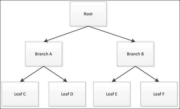
FIGURE 3-1: A tree in Python looks much like the physical alternative.
Note that the tree has just one root node — just as with a physical tree. The root node provides the starting point for the various kinds of processing you perform. Connected to the root node are either branches or leaves. A leaf node is always an ending point for the tree. Branch nodes support either other branches or leaves. The type of tree shown in Figure 3-1 is a binary tree because each node has, at most, two connections.
In looking at the tree, you see that Branch B is the child of the Root node. That's because the Root node appears first in the list. Leaf E and Leaf F are both children of Branch B, making Branch B the parent of Leaf E and Leaf F. The relationship between nodes is important because discussions about trees often consider the child/parent relationship between nodes. Without these terms, discussions of trees could become quite confusing.
Building a tree
Python doesn’t come with a built-in tree object. You must either create your own implementation or use a tree supplied with a library. A basic tree implementation requires that you create a class to hold the tree data object. The following code shows how you can create a basic tree class:
class binaryTree:
def __init__(self, nodeData, left=None, right=None):
self.nodeData = nodeData
self.left = left
self.right = right
def __str__(self):
return str(self.nodeData)
All this code does is create a basic tree object that defines the three elements that a node must include: data storage; left connection; and right connection. Because leaf nodes have no connection, the default value for left and right is None. The class also includes a method for printing the content of nodeData so that you can see what data the node stores.
Using this simple tree requires that you not try to store anything in left or right other than a reference to another node. Otherwise, the code will fail because there isn't any error trapping. The nodeData entry can contain any value. The following code shows how to use the binaryTree class to build the tree shown in Figure 3-1:
tree = binaryTree("Root")
BranchA = binaryTree("Branch A")
BranchB = binaryTree("Branch B")
tree.left = BranchA
tree.right = BranchB
LeafC = binaryTree("Leaf C")
LeafD = binaryTree("Leaf D")
LeafE = binaryTree("Leaf E")
LeafF = binaryTree("Leaf F")
BranchA.left = LeafC
BranchA.right = LeafD
BranchB.left = LeafE
BranchB.right = LeafF
You have many options when building a tree, but building it from the top down (as shown in this code) or the bottom up (in which you build the leaves first) are two common methods. Of course, you don't really know whether the tree actually works at this point. Traversing the tree means checking the links and verifying that they actually do connect as you think they should. The following code shows how to use recursion (as described in Book 2, Chapter 2) to traverse the tree you just built.
def traverse(tree):
if tree.left != None:
traverse(tree.left)
if tree.right != None:
traverse(tree.right)
print(tree.nodeData)
traverse(tree)
As the output shows, the traverse function doesn’t print anything until it gets to the first leaf:
Leaf C
Leaf D
Branch A
Leaf E
Leaf F
Branch B
Root
The traverse function then prints both leaves and the parent of those leaves. The traversal follows the left branch first, and then the right branch. The root node comes last.
 Trees have different kinds of data storage structures. Here is a quick list of the kinds of structures you commonly find:
- Balanced trees: A kind of tree that maintains a balanced structure through reorganization so that it can provide reduced access times. The number of elements on the left side differs from the number on the right side by at most one.
- Unbalanced trees: A tree that places new data items wherever necessary in the tree without regard to balance. This method of adding items makes building the tree faster but reduces access speed when searching or sorting.
- Heaps: A sophisticated tree that allows data insertions into the tree structure. The use of data insertion makes sorting faster. You can further classify these trees as max heaps and min heaps, depending on the tree's capability to immediately provide the maximum or minimum value present in the tree.
Representing Relations in a Graph
Graphs are another form of common data structure used in algorithms. You see graphs used in places like maps for GPS and all sorts of other places where the top-down approach of a tree won’t work. The following sections describe graphs in more detail.
Going beyond trees
A graph is a sort of tree extension. As with trees, you have nodes that connect to each other to create relationships. However, unlike binary trees, a graph can have more than one or two connections. In fact, graph nodes often have a multitude of connections. To keep things simple, though, consider the graph shown in Figure 3-2.
In this case, the graph creates a ring where A connects to both B and F. However, it need not be that way. Node A could be a disconnected node or could also connect to C. A graph shows connectivity between nodes in a way that is useful for defining complex relationships.
Graphs also add a few new twists that you might not have thought about before. For example, a graph can include the concept of directionality. Unlike a tree, which has parent/child relationships, a graph node can connect to any other node with a specific direction in mind. Think about streets in a city. Most streets are bidirectional, but some are one-way streets that allow movement in only one direction.
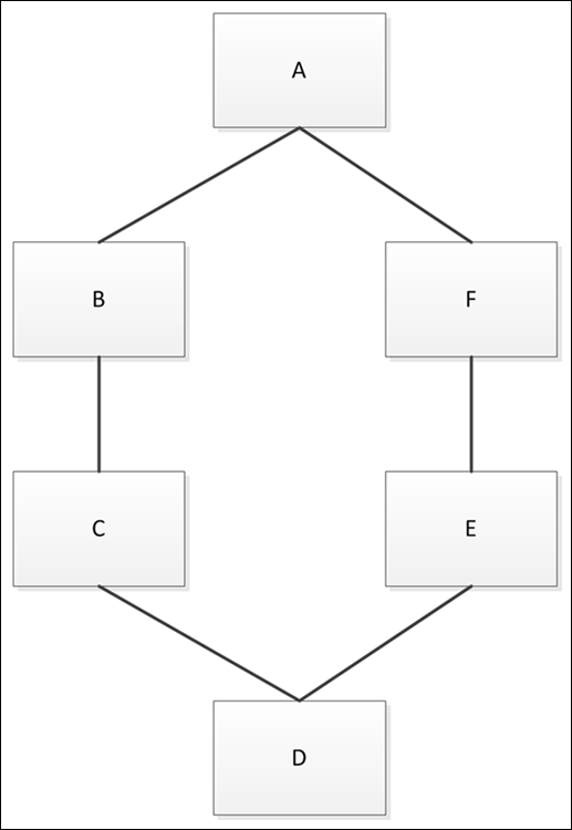
FIGURE 3-2: Graph nodes can connect to each other in myriad ways.
The presentation of a graph connection might not actually reflect the realities of the graph. A graph can designate a weight to a particular connection. The weight could define the distance between two points, define the time required to traverse the route, or provide other sorts of information.
Arranging graphs
Most developers use dictionaries (or sometimes lists) to build graphs. Using a dictionary makes building the graph easy because the key is the node name and the values are the connections for that node. For example, here is a dictionary that creates the graph shown in Figure 3-2:
graph = {'A': ['B', 'F'],
'B': ['A', 'C'],
'C': ['B', 'D'],
'D': ['C', 'E'],
'E': ['D', 'F'],
'F': ['E', 'A']}
This dictionary reflects the bidirectional nature of the graph in Figure 3-2. It could just as easily define unidirectional connections or provide nodes without any connections at all. However, the dictionary works quite well for this purpose, and you see it used in other areas of the book. Now it’s time to traverse the graph using the following code:
def find_path(graph, start, end, path=[]):
path = path + [start]
if start == end:
print("Ending")
return path
for node in graph[start]:
print("Checking Node ", node)
if node not in path:
print("Path so far ", path)
newp = find_path(graph, node, end, path)
if newp:
return newp
find_path(graph, 'B', 'E')
This simple code does find the path, as shown in the output:
Checking Node A
Path so far ['B']
Checking Node B
Checking Node F
Path so far ['B', 'A']
Checking Node E
Path so far ['B', 'A', 'F']
Ending
['B', 'A', 'F', 'E']
Other strategies help you find the shortest path (see Algorithms For Dummies, by John Paul Mueller and Luca Massaron [Wiley] for details on these techniques). For now, the code finds only a path. It begins by building the path node by node. As with all recursive routines, this one requires an exit strategy, which is that when the start value matches the end value, the path ends.
Because each node in the graph can connect to multiple nodes, you need a for loop to check each of the potential connections. When the node in question already appears in the path, the code skips it. Otherwise, the code tracks the current path and recursively calls find_path to locate the next node in the path.