
9
Scheduling of Robotic Disassembly in Remanufacturing Using Bees Algorithms
Jiayi Liu1, Wenjun Xu1, Zude Zhou1, and Duc Truong Pham2
1 School of Information Engineering, Wuhan University of Technology, Wuhan, China
2 Department of Mechanical Engineering, University of Birmingham, Birmingham, UK
9.1 Introduction
Low resource utilization and high environmental pollution are the major deficiencies of traditional manufacturing. It is said that in China, there are approximately 20 million mobile phones and 5 million cars scrapped every year [1]. Improper handling of end‐of‐life (EOL) products will cause resource‐wasting and environmental pollution [2]. Given this situation, remanufacturing is studied to protect the environment and to save manufacturing resources by making full use of EOL products [3]. It takes both economic development and environmental protection into considerations by reusing the EOL products [4]. In the remanufacturing process, it is necessary to consider the disassembly process to obtain the high‐value components. However, the disassembly process is usually executed by manual labor due to its high complexity. Robotic disassembly is recently being paid great attention because of the high automation potential. The cognitive robotics [5], its basic behavior control strategy [6], and learning/revision strategies [7] have been studied to realize the automated process of disassembling the screens.
Scheduling of robotic disassembly can reduce the cost and improve the efficiency of disassembly. Robotic disassembly cells (RDCs) and robotic disassembly lines (RDLs) are two major ways to disassemble EOL products. Scheduling of robotic disassembly mainly contains robotic disassembly sequence planning (RDSP) for an RDC and robotic disassembly line balancing problem (RDLBP) for an RDL. Considering disassembly precedence relationships of EOL products, finding the optimal disassembly sequences for RDCs is the purpose of RDSP [8]. In an RDL, the aim of RDLB is to assign appropriate disassembly tasks to robotic workstations to ensure even distribution of work among them [9]. Finding optimal solutions for RDSP and RDLB problems is important to improve disassembly efficiency.
RDSP and RDLBP are different from manual disassembly sequence planning (MDSP) and the manual disassembly line balancing problem (MDLBP). The moving time between different disassembly points (DPs) is always ignored in manual disassembly while in robotic disassembly it should not be ignored and can be determined by the end‐effector's moving speed and the length of the movement. In addition, the end‐effector should also avoid collisions with the product being disassembled.
The Bees algorithm mimics honeybees' foraging behavior and it has been applied to plenty of research fields, such as service aggregation optimization [10], image segmentation [11], and project scheduling [12]. It has been proved that Bees algorithms (BA) are highly competitive compared to the other methods [10]. However, little research has been conducted to solve the scheduling of robotic disassembly using a Bees algorithm.
In this chapter, scheduling of robotic disassembly (both RDSP [8] and RDLBP [9]) was solved by a Bees algorithm. The major contribution of this chapter is to consider the end‐effector's movement characteristics, and the moving time caused by the end‐effector's movement of different DPs is considered in the scheduling of robotic disassembly (both RDSP and RDLBP). Compared with the traditional methods, the optimal solutions of proposed methods obtained are more suitable for use in robotic disassembly. The related works are described in Section 9.2. Section 9.3 establishes the disassembly model. Consideration of the safe distance, the length of the obstacle‐avoiding path built, and the optimization objectives of RDSP and RDLBP are also described in Section 9.4. In Section 9.5, BA are used to search for the optimal solutions of RDSP and RDLBP. Case studies are conducted to verify the proposed methods in Section 9.6. Finally, Section 9.7 concludes this chapter.
9.2 Related Works
Scheduling of robotic disassembly mainly includes RDSP for an RDC and RDLBP for an RDL. Much research has been conducted in disassembly sequence planning (DSP) and disassembly line balancing problem (DLBP) fields.
Under given optimization objectives, finding the optimal disassembly sequence of EOL products is the purpose of DSP. Xing et al. [13] considered the disassembly distance, the disassembly direction changes, and the length of disassembly sequence, then they used the ant colony optimization algorithm to get the optimal solutions. Kheder et al. [14] used the genetic algorithm to get the optimal solutions of a rear axle. Jin et al. [15] used a brute‐force method to get the optimal solutions of disassembling the waste electrical and electronic equipment. Meng et al. [16] used an improved co‐evolutionary algorithm to simultaneously optimize the recovery options and disassembly level. For parallel and selective disassembly, Kim et al. [17] minimized the sequence‐dependent set‐ups and the operation cost of disassembly process using a branch and bound algorithm. When RDSP is studied, the end‐effector's movement characteristics should be considered. The total disassembly time consists of the basic disassembly time, the direction‐change time, the tool‐change time, and the moving time of robot's end‐effector between different DPs [18]. For robotic disassembly, the optimal solutions of disassembling personal computers were generated using a genetic algorithm [19]. Then DSP was solved using an online genetic algorithm to disassemble the same personal computers [20]. However, the end‐effector's moving time was computed using the end‐effector's moving speed and Euclidean distance between different DPs. For the practical robotic disassembly, the end‐effector's moving path cannot be a straight‐line path. The reason is that the end‐effector needs to move along the obstacle‐avoiding path to avoid physical collisions with the contour of EOL products. Thus, the existing methods used for DSP are not applicable to RDSP.
A disassembly line contains some disassembly workstations, and balancing the workstations' workload in a disassembly line is the optimization objective of DLBP. McGovern et al. [21] have proven that the decision version of DLBP is NP‐complete problems and its optimization version is NP‐hard problem. The linear physical programming was utilized by Ilgin et al. [22] to balance the disassembly line used for disassembling the smartphones. To disassemble cell phones, Ding et al. [23] minimized the demand rating, workstation number, and the balance measure using the ant colony algorithm. To optimize the design cost of a disassembly line, Ayyuce et al. [24] utilized a genetic algorithm to get the optimal solutions of stochastic DLBP. Bentaha et al. [25] solved DLBP, of which the disassembly task time was described by known probability distributions using the sample average approximation method and stochastic linear mixed‐integer programming. To get optimal solutions of DLBP using reasonable computation time, Mete et al. [26] minimized the workstation number of a disassembly line using the beam search algorithm. Nowadays, more attention has been paid to sequence‐dependent DLBP in which, if component A interacts with component B, extra time should be added. To solve sequence‐dependent DLBP, ant colony optimization [27], particle swarm optimization algorithm [28], improved artificial bee colony algorithm [29], hybrid genetic algorithm [30], and tabu search [31] were used to minimize the workstation number, the hazardous rating, the demand rating, and the balancing measures. The RDL is different from manual disassembly line in which the moving time between different DPs for each workstation is always ignored. In RDLBP, for each robotic workstation, EOL products can be the obstacles along the end‐effector's moving path. However, the existing research always ignores this and is not applicable to RDLBP.
Many metaheuristic algorithms are utilized to get the optimal solutions of DSP and DLBP. To disassemble machine vises, Xu et al. [32] solved DSP using the adaptive particle swarm optimization algorithm of which the mutation probability and inertia weight were adaptively determined. Luo et al. [33] obtained the optimal disassembly sequences of single‐speed reduction gearbox using multi‐layer representation method and ant colony optimization algorithm. For the U‐shaped disassembly line, optimal solutions of RDLBP were obtained by Agrawal et al. [34] using collaborative ant colony algorithm. To solve DLBP with a fixed workstation number, Kalaycılar et al. [35] maximized the total net revenue using upper and lower bounding procedures to assign suitable disassembly tasks to the workstations. The profit‐oriented partial DLBP was studied by Ren et al. [2] using an improved gravitational search algorithm. BA mimics honeybees' foraging behavior to get the optimal solutions and it is successfully applied to many research fields. Xu et al. [10] solved the service aggregation optimization problems using an improved BA. BA has also been applied to a fast scheme for multi‐level image thresholding of image segmentation [11]. Oztemel et al. [12] solved the resource‐constrained project scheduling problem in the mold industry using BA. The Bees algorithm has shown its great competitiveness compared with the other optimization algorithms [10], but it has not been applied to the scheduling of robotic disassembly yet.
9.3 Disassembly Model
To build the disassembly model, the disassembly precedence relationships of EOL products should be described. Many researchers either ignore the disassembly directions of components [23] or used the fixed disassembly direction to describe the disassembly directions of components [16]. Disassembly directions of components should be provided for the robots. The disassembly direction of components is not fixed and it should depend on the disassembly status of the other components [8]. Space interference matrix can be used to generate feasible disassembly directions of components according to the disassembly status of the other components [8]. In this chapter, the disassembly model is established.
9.3.1 Space Interference Matrix
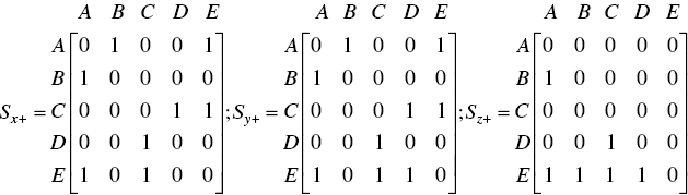
The space interference matrix Sod along orthogonal directions should be built first [15]. In Sod, each element smn represents when component n exists, whether component m could be disassembled along od direction or not. smn = 0 means component m could be disassembled along od direction if component n is not disassembled. Otherwise, smn = 1. The space interference matrices are built using an example as represented in Figure 9.1.

Figure 9.1 An example for space interference matrix.
This assembly's space interference matrices are represented by Eq. (9.1). In matrix Sz+, sCE is equal to 0. Although bolt C contacts component E, unscrewing operations along z + direction could be applied to bolt C to realize disassembly. In matrix Sz‐, sEC is equal to 1. The reason is that before bolt C is disassembled, component E cannot not be disassembled in the z – direction.

9.3.2 Interference Matrix Analysis
Feasible disassembly sequences are generated using interference matrix analysis. First, as represented by Eq. (9.2), space interference matrices (Sx±, Sy±, and Sz±) along orthogonal directions are combined into matrix Sx,y,z . From Eq. (9.2), the first element of column result in matrix Sx,y,z is 111101. The “OR” operator is applied to the first row of all the six interference matrices to get this element, which contains 6 bits. Only the fifth bit of this element is 0, it represents the fact that the corresponding component could be removed along the z + direction. It is apparent that both bolts A and C could be removed along the z + direction as represented by Eq. (9.2). If bolt A is randomly selected and disassembled along the z + direction, the first row and the first column of matrix Sx,y,z should be deleted as shown by Eq. (9.3). It is apparent that component B could be disassembled along any direction except the z − direction, as represented by Eq. (9.3). Component C could be removed along only the z + direction. Here, it is randomly selected and disassembled along the z + direction. After that, from Eq. (9.4), it is apparent that both components B and D could be disassembled along any direction except the z − direction, component E could be disassembled along x ± and y − directions. If component B is randomly selected and disassembled along y + direction, according to the same rule as represented by Eq. (9.5), matrix Sx,y,z should be updated. As represented by Eq. (9.5), component D could be disassembled along any direction except the z‐ direction, component E can be disassembled along x ± and y − directions. If component E is randomly selected and disassembled along x + direction, component D could be disassembled along any direction (x + direction is randomly selected). Thus, A/C/B/E/D and z+/z+/y+/x+/x + are the feasible solutions.


9.4 Optimization Objective
For RDC, finding the optimal disassembly sequences of EOL products helps to improve the disassembly efficiency of RDC, which is the core purpose of RDSP. Besides, RDL is the flow‐oriented product system, which includes some robotic workstations. It continuously launches the disassembly tasks down the disassembly line and EOL products are sequentially handled from one to another. Disassembly operations are repeatedly executed in each robotic workstation within the cycle time of RDL. RDLBP is the decision problem of balancedly assigning disassembly tasks to robotic workstations. Optimization objectives of both RDSP and RDLBP should be determined in advance.
In this chapter, the following assumptions are made: (i) the EOL products' structure and geometric information are known in advance; (ii) all parts in the EOL products can be disassembled; (iii) the EOL products are used for complete disassembly; (iv) the basic disassembly time, direction‐change time, and tool‐change time are constant and deterministic; (v) each disassembly task is assigned to only one robotic workstation in the RDL; and (vi) the total working time of robotic workstation is no greater than the cycle time of RDL.
9.4.1 The End‐effector's Moving Time
The end‐effector's moving time should not be ignored in robotic disassembly. Strictly, the obstacle‐avoiding path and the collision‐free trajectory should be considered [36]. The end‐effector's moving time should be determined by the position and complexity of products and the robot types. In this chapter, the moving time is generated by the moving path length and the end‐effector's velocity.
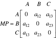
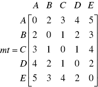
A simple example is illustrated here to represent the calculation process of the moving time between different DPs as shown in Figure 9.2. First, it should be ensured that there are no collisions. The black dotted line is the end‐effector's moving path as represented in Figure 9.2. Besides, the length matrix MP which represents the moving path length is denoted by Eq. (9.6). For example, the moving path length between DPs A and B is expressed as a12, which is calculated by Eq. (9.7). After matrix MP is decided, Eq. (9.8) is utilized to compute the moving time, where vee is the end‐effector's linear velocity.
Figure 9.2 An example to calculate the moving path between different DPs.
9.4.2 Optimization Objectives of RDSP
For RDC, minimizing the disassembly time of an EOL product is the optimization objective of RDSP. It mainly consists of the basic disassembly time, direction‐change time, tool‐change time, and the end‐effector's moving time.
The time used for disassembling a component using the robots is the basic disassembly time. To cope with the direction changes for the robots, extra time is needed to adjust its posture. The direction‐change time is expressed by Eq. (9.9). Similarly, the robot also needs extra disassembly time to handle disassembly tool changes. As shown in Figure 9.3, different disassembly tools correspond to different disassembly operations. The tool‐change time is represented by Eq. (9.10) where Scd, Spn, Pli, Grp, Elc, and Ham respectively indicate screwdriver, spanner, plier, gripper, electrical cutting and hammer. For the same operations, different disassembly tools (subclass) should also be included to disassemble different component types as represented by Eq. (9.11). For instance, different types of bolts should be disassembled by suitable types of spanners. The end‐effector's moving time is represented in Section 9.4.1.
Figure 9.3 Disassembly operations and tools.


Minimizing the disassembly time of an EOL product is the optimization objective which is expressed by Eq. (9.12), where X is the feasible disassembly sequence, n is the part number of EOL products, and bt(xi) represents the basic disassembly time of part xi . The tool‐change time, direction‐change time, and the end‐effector's moving time between parts xi and xi + 1 are respectively represented by tt(xi, xi + 1 ), dt(xi, xi + 1) and mt(xi, xi + 1 ).

The process of calculating the fitness value of a given feasible disassembly sequence is described using an example here. The feasible disassembly solution is A/C/B/E/D and x+/z+/x+/x+/z+, the corresponding disassembly tool is Td/Ta/Ta/Te/Td (spanner‐I, spanner‐II, spanner‐III, gripper‐I, and gripper‐II are respectively represented by Ta, Tb, Tc, Td, and Te). The tool‐change time and direction‐change time are respectively represented by Eqs. (9.9) and (9.13). Eq. (9.14) calculates the end‐effector's moving time. In this chapter, the basic disassembly time is assumed to be constant. The variable parameters are the latter three factors of Eq. (9.12). The fitness value of this feasible disassembly sequence could be calculated by Eq. (9.15).


9.4.3 Optimization Objectives of RDLBP
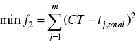
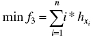
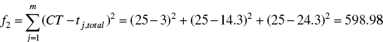
As represented by Eqs. (9.16)–(9.18), minimizing the robotic workstation number (f1 ), balancing the robotic workstation's workload (f2 ), and disassembling high demand parts as early as possible (f3) are the optimization objectives used in this chapter. Minimizing optimization objectives f1 and f2 respectively can reduce the cost and balance the robotic workstation's workload. Minimizing the optimization objective f3 helps to protect high‐demand parts from damage in the robotic disassembly process.
subject to:
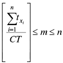
In Eqs. (9.16)–(9.22), m, n, hxi, and tj,total respectively indicate the robotic workstation number, part number of EOL products, the demand value of part xj and the jth robotic workstation's total working time. The cycle time CT is a predefined parameter in this chapter. X and FX respectively indicate the feasible disassembly sequence and feasible disassembly sequence set. Eqs. (9.19) and (9.20) respectively ensure the disassembly sequence is feasible and the robotic workstation number is limited within permitted values. Eqs. (9.21) and (9.22) respectively indicate that the total of any robotic workstation's working time should be no greater than the cycle time of RDL and a task is only assigned to a workstation.
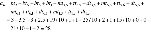
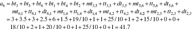
Feasible solutions of RDL should be obtained by the following method. Based on a given feasible disassembly sequence, an example is illustrated to generate the feasible disassembly solution and calculate its multi‐objective values. Table 9.1 lists the properties of the given disassembly sequence “3‐5‐6‐1‐4‐2‐7‐8” and the CT of RDL is 25 s. The direction‐change time, tool‐change time, and the length matrix MP are respectively represented by Eqs. . As represented in Figure 9.4, robotic workstations are assigned different disassembly tasks using the allocation matrix A = [ai ]. As shown in step 1, a4 and a6 are respectively calculated by Eqs. (9.25) and (9.26). It is obvious that a3 is less than CT (25 s) and a4 is greater than CT, which means robotic workstation 1 is assigned parts 3, 5, and 6. Then parts 3, 5, and 6 should be deleted and the disassembly sequence should be “1‐4‐2‐7‐8”. In step 2, the allocation matrix is obtained in the same manner. The former three elements in the allocation matrix are less than CT, which means robotic workstation 2 is assigned parts 1, 4, and 2. Similarly, in step 3, robotic workstation 3 is assigned parts 7 and 8. Finally, the multi‐objective values of this solution are calculated by Eqs. (9.27)–(9.29).

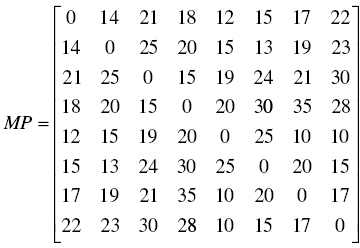
Table 9.1 Properties of a given disassembly sequence.
| Disassembly sequence | 3 | 5 | 6 | 1 | 4 | 2 | 7 | 8 |
| Basic disassembly time | 3 | 3.5 | 3 | 2.5 | 6 | 1.5 | 2 | 1.5 |
| Disassembly direction | z+ | y+ | x− | x− | z+ | y+ | x+ | x+ |
| Disassembly tool | Tb | Ta | Td | Td | Tb | Tb | Ta | Td |
| hxi | 2 | 3 | 3 | 1 | 4 | 2 | 3 | 2 |
| End‐effector's moving speed | 10 cm/s | |||||||

Figure 9.4 The robotic workstation assignment method for RDLBP.

9.5 Bees Algorithm
9.5.1 The Basic BA
BA mimics honeybees' foraging behavior to get optimal solutions [37]. In basic BA, several parameters are used: number of scout‐bees scoutn, number of selected sites m, number of elite sites n, number of follower bees of selected site mb, number of follower bees of elite sites nb, patch size ngh and iteration number iter. As shown in Figure 9.5, the solution space is randomly searched by scoutn scout bees. The visited sites' fitness values are computed and then sorted in ascending order. The best m and n sites are regarded as “selected sites” and “elite sites” respectively. The neighborhood space of each elite (non‐elites selected) site is searched by nb (mb) follower bees. If the quality of the newly searched site is better than the original one, the follower bee will replace this scout bee. Otherwise, this scout bee remains unchanged. After that, the remaining scoutn – m non‐selected sites are randomly searched as the global search strategy. All the scoutn sites should be sorted by the fitness values in ascending order and the next iteration process starts. When the current iteration number is larger than iter, the iteration process stops. Finally, the best bee in the scoutn scout Bees is regarded as the best solution.
Figure 9.5 The flowchart of basic BA.
9.5.2 Enhanced Discrete Bees Algorithm
RDSP is a combinatorial optimization problem and solved by enhanced discrete Bees algorithm (EDBA) in this chapter. The parameters scoutn, m, b, mb, nb, and iter of EDBA are similar to those of basic BA. Then, the disassembly model mentioned in Section 9.3 is utilized to generate scoutn feasible disassembly sequences which are regarded as scoutn scout bees of EDBA in Section 9.5.2.1. The nectar source (sites) are randomly searched and these sites are sorted by fitness values in ascending order. The best n and m sites are regarded as “elite sites” and “selected sites” respectively. The neighborhood space of each elite (non‐elite selected) site is searched by nb (mb) follower bees using the neighborhood search strategy. The best bee in the nb (mb) follower bees is selected and it is mutated using the mutation operator, namely, mutated bee. The mutated bee will replace the best bee if it is superior to the best bee. Otherwise, the best bee remains unchanged. The best bee will replace the original bee if the best bee is superior to the original scout bee. Otherwise, the original scout bee remains unchanged. The scoutn – m non‐selected sites are replaced by scoutn – m new sites. Then, all the visited sites are sorted by fitness values in ascending order, and the next iteration starts. When the current iteration number is larger than iter, the iteration process stops. Figure 9.6 describes the flowchart of EDBA.
9.5.2.1 Representation of Bees
Figure 9.7 represents a bee. The disassembly sequence and disassembly direction arrays are generated using the method mentioned in Section 9.3, and the disassembly tool and disassembly moving time arrays can be determined accordingly. Finally, the fitness value of a bee is calculated using the method mentioned in Section 9.4.2.
9.5.2.2 Neighborhood Search Strategy
The neighborhood search strategy which contains insert and swap operators is described in Figure 9.8.
When the swap operator is used, two integer numbers which indicate the swapping locations of the bee are randomly generated. Then, the corresponding two bits will be exchanged to be a new bee as represented in Figure 9.8a. From Figure 9.8b, one bit is randomly selected and it inserts a random location of a bee for the insert operator.
For both swap and insert operators, the newly generated solutions may be the infeasible disassembly sequence. The new bee's feasibility should be checked after this new bee is generated. If the new solution is infeasible, the original site's neighborhood should be searched until the new solution is feasible.
9.5.2.3 Mutation Operator
A component may be disassembled along several disassembly directions during the disassembly process. As represented in Figure 9.9, a mutation operator is utilized in this chapter to increase the solution diversity. When a mutation operator is used, one bit of disassembly direction array of a bee is randomly selected and it changes 180° (for example, from +y direction to −y direction). Besides, the new bee's feasibility also needs to be checked.

Figure 9.6 The flowchart of EDBA.

Figure 9.7 Representation of a bee in EDBA.

Figure 9.8 Neighborhood search strategy of EDBA: (a) swap operator and (b) insert operator.
Figure 9.9 Mutation operator.
9.5.2.4 Global Search Strategy
To avoid getting trapped in local optimum, scoutn – m non‐selected sites should be replaced by scoutn – m new sites using the method mentioned in Section 9.3.
9.5.3 Improved Multi‐Objective Discrete Bees Algorithm
An improved multi‐objective discrete Bees algorithm (IMODBA) is utilized to solve RDLBP and its flowchart is represented in Figure 9.10. Firstly, parameters scoutn, m, mb, and iter are initialized. Scout bees randomly explore the solution space and multi‐objective values of the visited sites are obtained. After that, efficient non‐dominated Pareto sorting method (ENS) and crowding‐distance method are utilized to sort the visited sites. Then the best m sites are chosen to be the “selected sites,” and the neighborhood of each selected site is searched by mb follower bees. The remaining scoutn‐m non‐selected sites are replaced by scoutn‐m new sites. At the end of each iteration process, scoutn + m*mb visited sites are sorted using ENS and crowding distance, the best scoutn bees are chosen for the next iteration process. When the current iteration number is larger than iter, the iteration process stops.
Figure 9.10 The flowchart of IMODBA.
9.5.3.1 Representation of Bees
Figure 9.11 describes a bee of IMODBA. The disassembly sequence and disassembly direction are obtained in the same manner as in Section 9.5.2.1. The robotic workstation array and multi‐objective value array are generated in the same manner as in Section 9.4.3.
9.5.3.2 Pareto Optimal Solution
In this chapter, minimizing the three objectives mentioned in Section 9.4.3 are the optimization objectives of RDLBP as represented by Eq. (9.30).
Suppose both X1 and X2 are feasible disassembly sequences, X2 is dominated by X1 if and only if Eq. (9.31) is satisfied:
Solution Xdom is Pareto optimal solution if no solutions dominate solution Xdom . The Pareto optimal set is made up of all the Pareto optimal solutions, and the function values of these Pareto optimal solutions are the Pareto optimal front.
9.5.3.3 Pareto Sorting
According to the dominance relationships between different solutions, assigning front ranks to all the solutions is the aim of Pareto sorting. ENS is used to be the Pareto sorting method of IMODBA [38]. The flowchart of ENS is described in Figure 9.12. More details can be found in Appendix A.
Figure 9.11 Representation of a bee in IMODBA.
Figure 9.12 The flowchart of ENS.
9.5.3.4 Crowding Distance Computation
To evaluate the solutions with the same front ranks, the crowding distance should be utilized [39]. For the solutions with the same front ranks, the solution with better crowding distance is preferable.
Figure 9.13 Computation process of crowding distance.
As represented in Figure 9.13, when the crowding distance is calculated, the solutions should be sorted according to the objective values in ascending order. For each objective value, the infinite distance value is assigned to the solutions with the largest and smallest objective values. The distance values of the intermediate solutions are calculated using the absolution normalized difference between two adjacent solutions' objective values. The solutions' crowding distance is obtained using the sum of the objectives' distance values.
9.5.3.5 Neighborhood Search Strategy
The sites' neighborhood is randomly explored by the follower bees. For IMODBA, mutation, insert, swap, and inverse operators are used to be the neighborhood search strategy as represented in Figure 9.14. The mutation operator acts on the disassembly direction. A random bit mutates and this bit changes 180° as represented in Figure 9.14a. The insert operator acts on both sequence and direction arrays, and a random bit inserts to a random position. The swap operator acts on both sequence and direction arrays. Two random bits are exchanged as represented in Figure 9.14c. The inverse operator also acts on both sequence and direction arrays, and a random part is inverted. Similar to the neighborhood search strategy of EDBA, if the new bees are unfeasible, the follower bees continue to search the neighborhood of scout bees until the new bees are feasible.

Figure 9.14 Neighborhood search strategy of IMODBA: (a) mutation operator, (b) insert operator, (c) swap operator, and (d) inverse operator.
9.6 Experiments and Results
9.6.1 Case Study
A gear pump is used to verify the proposed methods. The gear pump and its exploded view are described in Figure 9.15. The workflows of RDSP and RDLBP are represented in Figure 9.16. The properties of gear pump's parts are listed in Table 9.2.
The safe distance between the end‐effector's moving path and the contour of EOL products is 10 mm. The length matrix MP (MP = [mpij ]) is manually calculated. For example, as shown in Figure 9.17, the length of obstacle‐avoiding path mp1,13 between Bolt A and Shaft B is calculated by Eq. (9.32).

Figure 9.15 The gear pump and its exploded view: (a) the gear pump and (b) exploded view of the gear pump.
Figure 9.16 The workflow of RDSP and RDLBP.
Table 9.2 Properties of the gear pump's parts.
| Parts | Disassembly tasks | Tools | Disassembly point (mm) | hxi | bt/s |
| 1 | Unscrewing the Bolt A | Spanner‐I | [49.4, −12.6, 105.5] | 1 | 3 |
| 2 | Unscrewing the Bolt B | Spanner‐I | [74.4, −12.6, 81] | 1 | 3 |
| 3 | Unscrewing the Bolt C | Spanner‐I | [74.4, −12.6, 45] | 1 | 3 |
| 4 | Unscrewing the Bolt D | Spanner‐I | [49.4, −12.6, 20.5] | 1 | 3 |
| 5 | Unscrewing the Bolt E | Spanner‐I | [24.4, −12.6, 45] | 1 | 3 |
| 6 | Unscrewing the Bolt F | Spanner‐I | [24.4, −12.6, 81] | 1 | 3 |
| 7 | Removing the Cover | Gripper‐II | [49.4, −20.6, 63] | 2 | 4 |
| 8 | Removing the Gasket | Gripper‐I | [49.4, 1.4, 105.5] | 2 | 3 |
| 9 | Removing the Gear A | Gripper‐I | [49.4, 3.4, 81] | 3 | 6 |
| 10 | Removing the Gear B | Gripper‐I | [49.4, 3.4, 45] | 3 | 6 |
| 11 | Removing the Shaft A | Gripper‐I | [49.4, −7.6, 81] | 1 | 4 |
| 12 | Removing the Base | Gripper‐II | [49.4, 49.4, 81] | 4 | 8 |
| 13 | Removing the Shaft B | Gripper‐I | [49.4, 152.4, 45] | 2 | 4 |
| 14 | Removing the Packing Gland | Gripper‐I | [49.4, 91.4, 45] | 2 | 2 |
| 15 | Unscrewing the Gland Nut | Spanner‐II | [49.4, 96.4, 45] | 1 | 3 |

Figure 9.17 The moving path between Bolt A and Shaft B.
9.6.2 Performance Analysis
Simulations were finished on a personal computer with 4 GB memory and 2.3 GHz Intel Core i5‐6200U CPU using Matlab 2014b software.
9.6.2.1 RDSP Using EDBA
The performance analysis of RDSP using EDBA contains the following parts: (i) performance analysis with respect to different parameters; (ii) result comparisons using different methods; (iii) comparative analysis using different optimization algorithms.
The parameters m, n, mb, nb were respectively 4, 1, 1, and 2. It assumes that the end‐effector's moving speed is 12 mm/s. The fitness value and running time under different populations (from 10 to 40) and different iterations (from 100 to 500) are compared. Simulations were run 10 times. It is obvious when the parameter scoutn is fixed, the running time improves linearly with the parameter iter, as represented in Figure 9.18a. When population and iteration numbers are respectively 10 and 100, EDBA has the worst performance as shown in Figure 9.18b. The reason is that low‐quality solutions are obtained using insufficient populations and iterations. However, it is apparent that the solution quality increases with the iterations and populations [8].
Alshibli et al. [40] utilized the Euclidean distance to obtain the moving path length between different DPs. The result (Result 1) obtained using this method is compared with that of the proposed method (Result 2). In this chapter, the near‐optimal solutions are compared instead of the real optimal solutions which are difficult to obtain. The parameters m, n, mb, nb, iter, and scoutn were 4, 1, 1, 2, 500, and 40, respectively. The simulation was run 1000 times. In these 1000 solutions, the near‐optimal solution is the solution with the minimum fitness values. As represented in Table 9.3 (“1” and “2” respectively represent “y+” and “y−”), Result 2 is apparently different from Result 1, which is generated by the method using the Euclidean distance. For the robot's end‐effector, it is not practical to move along the straight line path using the result obtained by the traditional method. Thus, the proposed method is more suitable for use in the robotic disassembly compared with the traditional method.
EDBA is also compared with the other three optimization algorithms. For EDBA and EDBA without mutation operator (EDBA‐WMO), parameters m, n, mb, nb were respectively 4, 1, 1, and 2. For the genetic algorithm with precedence preserve crossover (GA‐PPX) [14], the mutation ratio was 0.1. For the self‐adaptive simplified swarm optimization (SASSO), Cp, Cg, and Cw were adaptively determined [41]. Each simulation was run 10 times. For the four optimization algorithms, the population number was 20, the results under different iterations are represented in Figure 9.19a and c. It is apparent that SASSO and GA‐PPX respectively need the most and the least running time of the four optimization algorithms. EDBA needs more running time compared with EDBA‐WMO. The reason is that more time needs to be spent on the mutation operators of EDBA. From Figure 9.19b and d, it is apparent that EDBA can find better solutions than the other three optimization algorithms. For the iteration process, the population and iteration numbers are respectively 20 and 300. From Figure 9.20, it is obvious that EDBA converges to the best solution of the four optimization algorithms.
Figure 9.18 Performance analysis of EDBA under different parameters: (a) average running time under different parameters of EDBA and (b) average fitness value under different parameters of EDBA.
Table 9.3 Comparisons of different results.
| Result 1 | Sequence | 5‐4‐3‐2‐1‐6‐7‐11‐8‐9‐10‐13‐15‐14‐12 |
| Direction | 2‐2‐2‐2‐2‐2‐2‐2‐2‐2‐2‐2‐1‐1‐1 | |
| Fitness | 58.5038 | |
| Result 2 | Sequence | 5‐4‐3‐2‐1‐6‐7‐10‐9‐11‐8‐13‐15‐14‐12 |
| Direction | 2‐2‐2‐2‐2‐2‐2‐2‐2‐2‐2‐2‐1‐1‐1 | |
| Fitness | 87.5731 |

Figure 9.19 Performance comparisons of four optimization algorithms: (a) average running time of four optimization algorithms under different iterations, (b) average fitness value of four optimization algorithms under different iterations, (c) average running time of four optimization algorithms under different populations, and (d) average fitness value of four optimization algorithms under different populations.
Figure 9.20 Iteration process of the four optimization algorithms.
9.6.2.2 RDLBP Using IMODBA
The performance analysis of IMODBA contains the following parts: (i) performance analysis with respect to different parameters; (ii) comparative analysis of different optimization algorithms; (iii) results comparison of different cases.
For the multi‐objective optimization algorithms, auxiliary methods should be utilized to assess the non‐dominated solutions' quality. In this chapter, generational distance (GD) [42] and hypervolume indicator (HI) [43] are used. The optimal Pareto solutions used to calculate the GD values are represented in Tables 9.6 and 9.7. The reference point used to calculate the HI values is set to [1.2, 1.2, 1.2]. Generally, lower GD values and greater HI values are preferable.
Before the GD and HI values of non‐dominated solutions are calculated, the multi‐objective values should be normalized by Eq. (9.33) where f1,min, f1,max, f2,min, f2,max, f3,min, and f3,max are 3, 5, 0.0548, 765.6372, 228, and 259, respectively.
For IMODBA, comparisons with respect to the running time, HI and GD values are made under different parameters. Parameters m and mb are respectively 15 and 1. It assumes that end‐effector's moving speed is 12 cm/s. Each simulation was run 50 times. As represented in Figure 9.21, IMODBA generates the best solutions (HI value is 1.5450 and GD value is 0.0080) when the parameters iter and scoutn are respectively 800 and 80, but it needs the most running time (67.55 s). When the parameters iter and scoutn are respectively 100 and 30, IMODBA generates the worst solutions (HI value is 1.4825 and GD value is 0.0149), but it needs the shortest running time (3.26 s) [9].
The comparative analysis of four optimization algorithms is conducted as follows.
- IMODBA: the proposed optimization algorithm in this chapter. The parameters mb and m are 1 and 15, respectively.
- MODBA: the fast nondominated sorting approach [39] is utilized. The parameters mb and m are 1 and 15, respectively.
- Multi‐objective artificial bees colony (MOABC): the onlooker bees, employed bees, and scout bees are utilized. The probability value of the onlooker bees is the same as the publication [44]. If a food source is not updated over 10 iterations, the employed bee will become the scout bee and new food source will be randomly explored.
- Multi‐objective genetic algorithm (MOGA): roulette wheel method, two‐point crossover procedure [45], and mutation procedure are utilized. The chromosome selection rate, mutation rate, and crossover rate are respectively 0.1, 0.2, and 0.8.
The results are compared with respect to iterations when parameter scoutn is 50 as represented in Figure 9.22. Each simulation was run 50 times. It is apparent that MODBA takes the most running time of the four optimization algorithms as represented in Figure 9.22a. IMODBA takes less running time than MODBA. Table 9.4 describes the running time improvement with respect to iterations. It is apparent that IMODBA and MODBA are superior to MOGA and MOABC in solution quality with respect to iterations, as represented in Figure 9.22c and e. IMODBA generates nearly the same quality of solutions compared with MODBA, the reason is that the solutions sorted by ENS are the same as the traditional methods while they are obtained using less running time. Simulations were conducted under different populations (from 30 to 80) when the iteration number is set to 500. Each simulation was run 50 times. The IMODBA generates optimal solutions using less time compared with MODBA and its running time is comparable with MOGA and MOABC as represented in Figure 9.22b. Table 9.5 describes the running time improvement with respect to populations. From Figure 9.22d and f, it is apparent that solution quality of IMODBA and MODBA is better than MOGA and MOABC under different populations. IMODBA generate nearly the same quality of solutions with MODBA, the reason is also that the solutions sorted by ENS are the same as the traditional methods.

Figure 9.21 Performance analysis of IMODBA under different parameters: (a) average running time of IMODBA under different parameters, (b) average HI values of IMODBA under different parameters, and (c) average GD values of IMODBA under different parameters.

Figure 9.22 Comparative analysis of different optimization algorithms: (a) average running time under different iterations, (b) average running time under different populations, (c) average HI values under different iterations, (d) average HI values under different populations, (e) average GD values under different iterations, and (f) average GD values under different populations.
Table 9.4 Running time improvement with respective to iterations.
| Iteration number | 100 | 200 | 300 | 400 | 500 | 600 | 700 | 800 |
| IMODBA | 5.31 s | 10.77 s | 15.71 s | 20.98 s | 26.18 s | 31.16 s | 36.55 s | 41.86 s |
| MODBA | 5.63 s | 11.57 s | 17.29 s | 22.93 s | 28.19 s | 33.54 s | 39.50s | 45.42 s |
| Improvement | 0.32 s | 0.80 s | 1.58 s | 1.95 s | 2.01 s | 2.38 s | 2.95 s | 3.56 s |
| Percentage | 5.68% | 6.91% | 9.14% | 8.50% | 7.13% | 7.10% | 7.47% | 7.84% |
Table 9.5 Running time improvement with respective to populations.
| Population number | 30 | 40 | 50 | 60 | 70 | 80 |
| IMODBA | 16.19 s | 21.41 s | 26.18 s | 31.38 s | 36.27 s | 40.92 s |
| MODBA | 17.83 s | 22.85 s | 28.19 s | 33.02 s | 38.14 s | 43.03 s |
| Improvement | 1.64 s | 1.44 s | 2.01 s | 1.64 s | 1.87 s | 2.11 s |
| Percentage | 9.20% | 6.30% | 7.13% | 4.97% | 4.90% | 4.90% |
Comparisons are also made with respect to Pareto optimal fronts using different cases as follows.
- Case 1: the basic disassembly time, direction‐change time and tool‐change time are considered, but the end‐effector's moving time is ignored in this case.
- Case 2: the end‐effector's moving time, the basic disassembly time, direction‐change time, and tool‐change time are considered. The end‐effector's moving time is calculated using the Euclidean distance.
- Case 3: the proposed method in this chapter is used.
It is hard to exhaust the solutions and obtain real optimal solutions. The near Pareto optimal solutions are generated in the following way. The scout bees number scoutn, the iteration number iter, the follower bees number mb of selected site, and the selected sites number m of IMODBA are 80, 800, 1, and 15, respectively. Simulations were run 100 times. The near Pareto optimal solutions are obtained by sorting these 100 groups of non‐dominated solutions. Table 9.6 does not list the Pareto fronts obtained by MODBA, the reason is that the solutions obtained by MODBA are the same with IMODBA. Pareto fronts generated by case 3 are apparently different from cases 1 and 2 as represented in Table 9.6. The end‐effector's moving time is ignored in case 1 and the obstacle caused by the EOL products is also ignored in case 2. Case 3 should be more applicable for RDLBP compared with cases 1 and 2. In addition, from case 3 in Table 9.6, the fourth and seventh solutions of IMODBA dominates the fourth and eighth solutions of MOABC respectively. The fifth solution obtained by IMODBA dominates the fifth and sixth solutions obtained by MOABC. IMODBA is also superior to MOGA in Pareto fronts number. Thus, IMODBA can generate better Pareto fronts compared with MOGA and MOABC. Table 9.7 lists the Pareto optimal solutions of RDLBP.
Table 9.6 Pareto fronts of three different cases.
| No. | Case 1 | Case 2 | Case 3 | ||||||||||||||||||||||||
| IMODBA | MOABC | MOGA | IMODBA | MOABC | MOGA | IMODBA | MOABC | MOGA | |||||||||||||||||||
| f1 | f2 | f3 | f1 | f2 | f3 | f1 | f2 | f3 | f1 | f2 | f3 | f1 | f2 | f3 | f1 | f2 | f3 | f1 | f2 | f3 | f1 | f2 | f3 | f1 | f2 | f3 | |
| 1 | 3 | 1 | 234 | 3 | 1 | 234 | 3 | 1 | 234 | 3 | 0.5262 | 238 | 3 | 0.5262 | 238 | 3 | 0.5262 | 238 | 3 | 0.0548 | 246 | 3 | 0.0548 | 246 | 3 | 0.0548 | 246 |
| 2 | 3 | 5 | 232 | 3 | 5 | 232 | 3 | 5 | 232 | 3 | 2.9193 | 235 | 3 | 2.9193 | 235 | 3 | 2.9193 | 235 | 3 | 0.0860 | 243 | 3 | 0.0860 | 243 | 3 | 0.0860 | 243 |
| 3 | 3 | 6 | 230 | 3 | 6 | 230 | 3 | 6 | 230 | 3 | 3.2023 | 234 | 3 | 3.2023 | 234 | 3 | 3.2023 | 234 | 3 | 0.1899 | 241 | 3 | 0.1899 | 241 | 3 | 0.1899 | 241 |
| 4 | 3 | 10 | 228 | 3 | 10 | 228 | 3 | 10 | 228 | 3 | 7.5069 | 233 | 3 | 7.5069 | 233 | 3 | 14.3724 | 232 | 3 | 1.0637 | 239 | 3 | 1.5690 | 240 | 3 | 2.0211 | 236 |
| 5 | 4 | 14.3724 | 232 | 3 | 14.3724 | 232 | 4 | 198.9339 | 231 | 3 | 2.0211 | 236 | 3 | 2.2897 | 238 | 3 | 3.8500 | 235 | |||||||||
| 6 | 4 | 198.9339 | 231 | 4 | 198.9339 | 231 | 4 | 251.9134 | 230 | 3 | 3.8500 | 235 | 3 | 3.6332 | 236 | 3 | 6.3106 | 233 | |||||||||
| 7 | 4 | 251.9134 | 230 | 4 | 251.9134 | 230 | 4 | 355.8085 | 229 | 3 | 6.3106 | 233 | 3 | 6.3106 | 235 | 4 | 27.0273 | 232 | |||||||||
| 8 | 4 | 355.8085 | 229 | 4 | 355.8085 | 229 | 4 | 448.1330 | 228 | 4 | 27.0273 | 232 | 4 | 26.9303 | 234 | 4 | 27.2973 | 231 | |||||||||
| 9 | 4 | 448.1330 | 228 | 4 | 448.1330 | 228 | 4 | 27.2973 | 231 | 4 | 27.0273 | 232 | 4 | 27.4623 | 230 | ||||||||||||
| 10 | 4 | 27.4623 | 230 | 4 | 27.2973 | 231 | 4 | 263.5929 | 229 | ||||||||||||||||||
| 11 | 4 | 263.5929 | 229 | 4 | 27.4623 | 230 | 4 | 284.1421 | 228 | ||||||||||||||||||
| 12 | 4 | 284.1421 | 228 | 4 | 263.5929 | 229 | |||||||||||||||||||||
| 13 | 4 | 284.1421 | 228 | ||||||||||||||||||||||||
Table 9.7 Pareto optimal solutions.
| Algorithms | No. | Sequence | Direction | Robotic workstation | f1 | f2 | f3 |
| IMODBA | 1 | 4‐5‐6‐2‐3‐1‐7‐15‐8‐14‐12‐9‐13‐11‐10 | 2‐2‐2‐2‐2‐2‐2‐1‐2‐1‐1‐2‐2‐1‐1 | 1‐1‐1‐1‐1‐1‐1‐2‐2‐2‐2‐3‐3‐3‐3 | 3 | 0.0548 | 246 |
| 2 | 4‐2‐3‐5‐6‐1‐7‐15‐8‐14‐12‐10‐9‐13‐11 | 2‐2‐2‐2‐2‐2‐2‐1‐2‐1‐1‐2‐1‐2‐2 | 1‐1‐1‐1‐1‐1‐1‐2‐2‐2‐2‐3‐3‐3‐3 | 3 | 0.0860 | 243 | |
| 3 | 4‐2‐3‐5‐6‐1‐7‐15‐14‐12‐8‐10‐9‐13‐11 | 2‐2‐2‐2‐2‐2‐2‐1‐1‐1‐2‐2‐1‐2‐2 | 1‐1‐1‐1‐1‐1‐1‐2‐2‐2‐2‐3‐3‐3‐3 | 3 | 0.1899 | 241 | |
| 4 | 15‐14‐3‐5‐4‐6‐1‐2‐7‐9‐8‐12‐13‐10‐11 | 1‐1‐2‐2‐2‐2‐2‐2‐2‐2‐2‐1‐1‐1‐1 | 1‐1‐1‐1‐1‐2‐2‐2‐2‐2‐2‐3‐3‐3‐3 | 3 | 1.0637 | 239 | |
| 5 | 15‐14‐13‐2‐6‐3‐5‐1‐4‐7‐8‐12‐10‐9‐11 | 1‐1‐1‐2‐2‐2‐2‐2‐2‐2‐2‐1‐1‐1‐1 | 1‐1‐1‐1‐1‐2‐2‐2‐2‐2‐2‐3‐3‐3‐3 | 3 | 2.0211 | 236 | |
| 6 | 1‐6‐5‐3‐2‐4‐7‐10‐9‐15‐14‐12‐8‐13‐11 | 2‐2‐2‐2‐2‐2‐2‐2‐2‐1‐1‐1‐1‐1‐1 | 1‐1‐1‐1‐1‐1‐1‐2‐2‐2‐2‐3‐3‐3‐3 | 3 | 3.8500 | 235 | |
| 7 | 15‐14‐13‐5‐6‐1‐2‐3‐4‐7‐9‐12‐10‐8‐11 | 1‐1‐1‐2‐2‐2‐2‐2‐2‐2‐2‐1‐1‐1‐1 | 1‐1‐1‐1‐1‐2‐2‐2‐2‐2‐2‐3‐3‐3‐3 | 3 | 6.3106 | 233 | |
| 8 | 15‐14‐3‐6‐13‐5‐1‐4‐2‐12‐9‐7‐8‐10‐11 | 1‐1‐2‐2‐1‐2‐2‐2‐2‐1‐1‐2‐1‐2‐1 | 1‐1‐1‐1‐2‐2‐2‐2‐3‐3‐3‐4‐4‐4‐4 | 4 | 27.0273 | 232 | |
| 9 | 15‐14‐3‐6‐13‐4‐1‐5‐2‐12‐9‐7‐10‐8‐11 | 1‐1‐2‐2‐1‐2‐2‐2‐2‐1‐1‐2‐1‐2‐1 | 1‐1‐1‐1‐2‐2‐2‐2‐3‐3‐3‐4‐4‐4‐4 | 4 | 27.2973 | 231 | |
| 10 | 15‐14‐5‐2‐13‐3‐1‐4‐6‐12‐9‐7‐8‐11‐10 | 1‐1‐2‐2‐1‐2‐2‐2‐2‐1‐1‐2‐1‐2‐1 | 1‐1‐1‐1‐2‐2‐2‐2‐3‐3‐3‐4‐4‐4‐4 | 4 | 27.4623 | 230 | |
| 11 | 15‐14‐13‐3‐4‐1‐5‐2‐6‐12‐9‐7‐10‐8‐11 | 1‐1‐1‐2‐2‐2‐2‐2‐2‐1‐1‐2‐1‐2‐1 | 1‐1‐1‐1‐2‐2‐2‐2‐2‐3‐3‐3‐4‐4‐4 | 4 | 263.5929 | 229 | |
| 12 | 15‐14‐13‐3‐4‐1‐5‐2‐6‐12‐9‐10‐7‐8‐11 | 1‐1‐1‐2‐2‐2‐2‐2‐2‐1‐1‐1‐2‐2‐1 | 1‐1‐1‐1‐2‐2‐2‐2‐2‐3‐3‐3‐4‐4‐4 | 4 | 284.1421 | 228 | |
| MOABC | 1 | 15‐14‐13‐6‐2‐3‐5‐1‐4‐7‐11‐12‐9‐10‐8 | 1‐1‐1‐2‐2‐2‐2‐2‐2‐2‐2‐1‐1‐1‐1 | 1‐1‐1‐1‐1‐2‐2‐2‐2‐2‐2‐3‐3‐3‐3 | 3 | 1.5690 | 240 |
| 2 | 15‐14‐13‐2‐3‐5‐1‐4‐6‐7‐8‐12‐10‐11‐9 | 1‐1‐1‐2‐2‐2‐2‐2‐2‐2‐2‐1‐1‐1‐1 | 1‐1‐1‐1‐1‐2‐2‐2‐2‐2‐2‐3‐3‐3‐3 | 3 | 2.2897 | 238 | |
| 3 | 15‐14‐13‐2‐3‐5‐6‐1‐4‐7‐8‐12‐10‐9‐11 | 1‐1‐1‐2‐2‐2‐2‐2‐2‐2‐2‐1‐1‐1‐1 | 1‐1‐1‐1‐1‐2‐2‐2‐2‐2‐2‐3‐3‐3‐3 | 3 | 3.6332 | 236 | |
| 4 | 15‐14‐3‐6‐13‐4‐1‐5‐2‐12‐9‐8‐7‐11‐10 | 1‐1‐2‐2‐1‐2‐2‐2‐2‐1‐1‐1‐2‐1‐2 | 1‐1‐1‐1‐2‐2‐2‐2‐3‐3‐3‐4‐4‐4‐4 | 4 | 26.9303 | 234 | |
| 5–13 | The 1st ~ 3rd and 7th ~ 12th solutions of IMODBA. | ||||||
| MOGA | 1–11 | The 1st ~ 3rd and 5th ~ 12th solutions of IMODBA. | |||||
9.7 Conclusion
Scheduling of robotic disassembly in remanufacturing mainly contains RDSP and RDLBP, which were respectively solved by EDBA and IMODBA. Disassembly precedence relationships of products were represented by a disassembly model. Including the safe distance, the moving time between different DPs was generated using the obstacle‐avoiding path length and the end‐effector's moving speed. After that, the optimization objectives of RDSP and RDLBP were also introduced. Then, two types of BA were developed to solve RDSP and RDLBP, namely, EDBA and IMODBA. Finally, a gear pump was utilized to verify the proposed methods. The results show that the proposed methods are more applicable to be used in the scheduling of robotic disassembly compared with the traditional methods. EDBA is superior to EDBA‐WMO, GA‐PPX, and SASSO in solution quality, while IMODBA is also superior to MOGA and MOABC in solution quality. The practical implication of this chapter is to provide guidance to generate the optimal disassembly solutions of disassembling EOL products for both RDCs and RDLs. However, there are also some limitations of the proposed methods. First, the disassembly model used in this chapter can only generate orthogonal disassembly directions for each component while in the practical robotic disassembly process, the disassembly directions of components should be more complex. Besides, the obstacle‐avoiding path length is manually obtained, it is time‐consuming and cumbersome for manual labor. In the future, methods of efficiently obtaining the obstacle‐avoiding path length should be studied. Besides, the disassembly process is full of uncertainties. This chapter assumes that disassembly time is constant and deterministic. In the future, we will study more practical methods which are applicable to handle the uncertainties in the robotic disassembly process.
Acknowledgments
This work was supported by National Natural Science Foundation of China (Grant Nos. 51775399 and 51475343), Engineering and Physical Sciences Research Council (EPSRC), UK (Grant No. EP/N018524/1), and the China Scholarship Council (CSC).
A. Appendix A
An example of ENS is illustrated here as follows. As shown in Figure 9.A1, for the given population P, the sorted population P* is obtained according to lexicographical order. In step 1, the front rank Fr1 is assigned to the 1st solution (solution 3) of the sorted population P *. In step 2, the 2nd solution of population P* is compared with the solutions with front rank Fr1 from the last to the first. It is obvious that solution 7 is not dominated by solution 3 and front rank Fr1 is assigned to solution 7. Then, comparisons are made between solution 6 and the solutions with front rank Fr1 from the last to the first. It is apparent that solution 7 dominates solution 6 and front rank Fr2 does not exist in set Fr. Thus, front rank Fr2 is created and it is assigned to the solution 6. Based on the same rules, through steps 4–8, all the solutions in sorted population P* are assigned the front ranks as shown in Figure 9.A1.

Figure 9.A1 An example to illustrate the process of ENS.
References
- 1 Xu, B.S. (2010). State of the art and future development in remanufacturing engineering. Trans. Mater. Heat Treatment 31 (1): 10–14.
- 2 Ren, Y.P., Yu, D.Y., Zhang, C.Y. et al. (2017). An improved gravitational search algorithm for profit‐oriented partial disassembly line balancing problem. Int. J. Prod. Res. 55 (24): 7302–7316.
- 3 Diallo, C., Venkatadri, U., Khatab, A., and Bhakthavatchalam, S. (2017). State of the art review of quality, reliability and maintenance issues in closed‐loop supply chains with remanufacturing. Int. J. Prod. Res. 55 (5): 1277–1296.
- 4 Guide, V.D.R. (2000). Production planning and control for remanufacturing: industry practice and research needs. J. Oper. Manage. 18 (4): 467–483.
- 5 Vongbunyong, S., Kara, S., and Pagnucco, M. (2012). A framework for using cognitive robotics in disassembly automation. Proceedings of the 19th CIRP International Conference on Life Cycle Engineering, 173–178.
- 6 Vongbunyong, S., Kara, S., and Pagnucco, M. (2013). Basic behaviour control of the vision‐based cognitive robotic disassembly automation. Assem. Autom. 33 (1): 38–56.
- 7 Vongbunyong, S., Kara, S., and Pagnucco, M. (2015). Learning and revision in cognitive robotics disassembly automation. Rob. Comput.‐Integr. Manuf. 34: 79–94.
- 8 Liu, J.Y., Zhou, Z.D., Pham, D.T. et al. (2018). Robotic disassembly sequence planning using enhanced discrete bees algorithm in remanufacturing. Int. J. Prod. Res. 56 (9): 3134–3151.
- 9 Liu, J.Y., Zhou, Z.D., Pham, D.T. et al. (2018). An improved multi‐objective discrete bees algorithm for robotic disassembly line balancing problem in remanufacturing. Int. J. Adv. Manuf. Technol. 97 (9–12): 3937–3962.
- 10 Xu, W.J., Tian, S.S., Liu, Q. et al. (2016). An improved discrete bees algorithm for correlation‐aware service aggregation optimization in cloud manufacturing. Int. J. Adv. Manuf. Technol. 84 (1–4): 17–28.
- 11 Hussein, W.A., Sahran, S., and Abdullah, S.N.H.S. (2016). A fast scheme for multilevel thresholding based on a modified bees algorithm. Knowl.‐Based Syst. 101: 114–134.
- 12Oztemel, E. and Selam, A.A. (2017). Bees algorithm for multi‐mode, resource‐constrained project scheduling in molding industry. Comput. Ind. Eng. 112: 187–196.
- 13 Xing, Y.F., Wang, C.E., and Liu, Q. (2012). Disassembly sequence planning based on Pareto ant Colony algorithm. J. Mech. Eng. 48 (9): 186–192.
- 14 Kheder, M., Trigui, M., and Aifaoui, N. (2015). Disassembly sequence planning based on a genetic algorithm. Proc. Inst. Mech. Eng., Part C: J. Mech. Eng. Sci. 229 (12): 2281–2290.
- 15 Jin, G.Q., Li, W.D., Wang, S., and Gao, S.M. (2017). A systematic selective disassembly approach for waste electrical and electronic equipment with case study on liquid crystal display televisions. Proc. Inst. Mech. Eng., Part B: J. Eng. Manuf. 231 (13): 2261–2278.
- 16 Meng, K., Lou, P.H., Peng, X.H., and Prybutok, V. (2016). An improved co‐evolutionary algorithm for green manufacturing by integration of recovery option selection and disassembly planning for end‐of‐life products. Int. J. Prod. Res. 54 (18): 5567–5593.
- 17 Kim, H.W. and Lee, D.H. (2017). An optimal algorithm for selective disassembly sequencing with sequence‐dependent set‐ups in parallel disassembly environment. Int. J. Prod. Res. 55 (24): 7317–7333.
- 18 ElSayed, A., Kongar, E., Gupta, S., and Sobh, T. (2011). An online genetic algorithm for automated disassembly sequence generation. In: ASME 2011 International Design Engineering Technical Conferences and Computers and Information in Engineering Conference, 657–664. Washington: American Society of Mechanical Engineers.
- 19 ElSayed, A., Kongar, E., and Gupta, S.M. (2010). A genetic algorithm approach to end‐of‐life disassembly sequencing for robotic disassembly. Proceedings of the 2010 Northeast Decision Sciences Institute Conference, Alexandria, VA, USA (26–28 March), 402–408.
- 20 ElSayed, A., Kongar, E., Gupta, S.M., and Sobh, T. (2012). A robotic‐driven disassembly sequence generator for end‐of‐life electronic products. J. Intell. Rob. Syst. 68 (1): 43–52.
- 21 McGovern, S.M. and Gupta, S.M. (2007). A balancing method and genetic algorithm for disassembly line balancing. Eur. J. Oper. Res. 179 (3): 692–708.
- 22 Ilgin, M.A., Akcay, H., and Araz, C. (2017). Disassembly line balancing using linear physical programming. Int. J. Prod. Res. 55 (20): 6108–6119.
- 23 Ding, L.P., Feng, Y.X., Tan, J.R., and Gao, Y.C. (2010). A new multi‐objective ant colony algorithm for solving the disassembly line balancing problem. Int. J. Adv. Manuf. Technol. 48 (5–8): 761–771.
- 24 Aydemir‐Karadag, A. and Turkbey, O. (2013). Multi‐objective optimization of stochastic disassembly line balancing with station paralleling. Comput. Ind. Eng. 65 (3): 413–425.
- 25 Bentaha, M.L., Battaia, O., and Dolgui, A. (2014). A sample average approximation method for disassembly line balancing problem under uncertainty. Comput. Oper. Res. 51: 111–122.
- 26 Mete, S., Cil, Z.A., Agpak, K. et al. (2016). A solution approach based on beam search algorithm for disassembly line balancing problem. J. Manuf. Syst. 41: 188–200.
- 27 Kalayci, C.B. and Gupta, S.M. (2013). Ant colony optimization for sequence‐dependent disassembly line balancing problem. J. Manuf. Technol. Manage. 24 (3): 413–427.
- 28 Kalayci, C.B. and Gupta, S.M. (2013). A particle swarm optimization algorithm with neighborhood‐based mutation for sequence‐dependent disassembly line balancing problem. Int. J. Adv. Manuf. Technol. 69 (1–4): 197–209.
- 29 Liu, J. and Wang, S.W. (2017). Balancing disassembly line in product recovery to promote the coordinated development of economy and environment. Sustainability 9 (2): 309–323.
- 30 Kalayci, C.B., Polat, O., and Gupta, S.M. (2016). A hybrid genetic algorithm for sequence‐dependent disassembly line balancing problem. Ann. Oper. Res. 242 (2): 321–354.
- 31 Kalayci, C.B. and Gupta, S.M. (2014). A tabu search algorithm for balancing a sequence‐dependent disassembly line. Prod. Plann. Control 25 (2): 149–160.
- 32 Xu, J., Zhang, S.Y., and Fei, S.M. (2011). Product remanufacture disassembly planning based on adaptive particle swarm optimization algorithm. J. Zhejiang Univ. Eng. Sci. 45 (10): 1746–1752.
- 33 Luo, Y., Peng, Q., and Gu, P. (2016). Integrated multi‐layer representation and ant colony search for product selective disassembly planning. Comput. Ind. 75: 13–26.
- 34 Agrawal, S. and Tiwari, M.K. (2008). A collaborative ant colony algorithm to stochastic mixed‐model U‐shaped disassembly line balancing and sequencing problem. Int. J. Prod. Res. 46 (6): 1405–1429.
- 35 Kalaycilar, E.G., Azizoglu, M., and Yeralan, S. (2016). A disassembly line balancing problem with fixed number of workstations. Eur. J. Oper. Res. 249 (2): 592–604.
- 36 Constantinescu, D. and Croft, E.A. (2000). Smooth and time‐optimal trajectory planning for industrial manipulators along specified path. J. Rob. Syst. 17 (5): 233–249.
- 37 Pham, Q.T., Pham, D.T., and Castellani, M. (2012). A modified bees algorithm and a statistics‐based method for tuning its parameters. Proc. Inst. Mech. Eng., Part I: J. Syst. Control Eng. 226 (3): 287–301.
- 38 Zhang, X.Y., Tian, Y., Cheng, R., and Jin, Y.C. (2015). An efficient approach to nondominated sorting for evolutionary multiobjective optimization. IEEE Trans. Evol. Comput. 19 (2): 201–213.
- 39 Deb, K., Pratap, A., Agarwal, S., and Meyarivan, T. (2002). A fast and elitist multiobjective genetic algorithm: NSGA‐II. IEEE Trans. Evol. Comput. 6 (2): 182–197.
- 40Alshibli, M., ElSayed, A., Kongar, E. et al. (2015). Disassembly sequencing using tabu search. J. Intell. Rob. Syst. 82 (1): 1–11.
- 41 Yeh, W.C. (2012). Optimization of the disassembly sequencing problem on the basis of self‐adaptive simplified swarm optimization. IEEE Trans. Syst., Man, Cybern. – Part A: Syst. Humans 42 (1): 250–261.
- 42 Okabe, T., Jin, Y., and Sendhoff, B. (2003). A critical survey of performance indices for multi‐objective optimisation. Proceedings of 2003 Congress on IEEE on Evolutionary Computation, Canberra, Australia (8–12 December), 878–885.
- 43 Zitzler, E., and Thiele, L. (1998). Multiobjective optimization using evolutionary algorithms—a comparative case study. Proceedings of 1998 International Conference on Parallel Problem Solving from Nature, Amsterdam, Netherlands (27–30 September), 292–301.
- 44 Akbari, R., Hedayatzadeh, R., Ziarati, K., and Hassanizadeh, B. (2012). A multi‐objective artificial bee colony algorithm. Swarm Evol. Comput. 2: 39–52.
- 45 Akpınar, S. and Bayhan, G.M. (2011). A hybrid genetic algorithm for mixed model assembly line balancing problem with parallel workstations and zoning constraints. Eng. Appl. Artif. Intell. 24 (3): 449–457.