5.1 Introduction and Problem Statement Formulation

In this section, different problem statements/scenarios of multi‐antenna wireless communication systems are discussed, where GA and PSO have been implemented to provide computationally efficient scheduling schemes. Also, an introduction to these problem statements/scenarios is presented for understanding the background.

Single‐antenna systems offer less system capacity as they can transmit data to only one user instantaneously. The system capacity enhancement of wireless systems and lower delay wireless packet data systems is achieved by multi‐user multiple‐input multiple‐output (MU‐MIMO) systems by transmitting data to several users, as many as the number of antennas at the base station (BS) without requiring additional bandwidth or transmit power. This simultaneous data transfer by BS to a number of users is proposed in a dirty paper coding (DPC) scheme. Hence, BS always searches for a subset of users who are the best in channel conditions. To accomplish this activity, BS needs full channel state information (CSI) of every user in the reverse channel according to DPC. DPC is an example of an extensive search scheme (ESS) which is hard to realize for a higher number of users and BS antennas due to the constraint in hardware implementation.

MIMO systems achieve higher system sum‐rate than single antenna systems by spatial multiplexing, where multiple parallel data streams can be transmitted from the transmitter to the receiver simultaneously. Multi‐user diversity (MUD) helps to achieve further gain in system sum‐rate for MU‐MIMO systems [1, 2]. This is because of independent and uncorrelated fading channels between the BS and various user equipment (UE) present at different geographical locations. In the broadcast channel (BC), the BS sends the data message to multiple UEs simultaneously according to DPC [3]. The number of simultaneously served UEs by the BS is equal to the number of antennas at the BS [4, 5]. Because of this, it becomes the duty of the BS to select/schedule M_T number of UEs among K UEs with the best channel parameters for getting service from the BS, where M_T is the number of antennas present at the BS. A variety of MU‐MIMO scheduling algorithms [6–10] have been proposed in literature, which take advantage of MUD.

Good cross‐layer scheduling schemes make both the physical layer and the multiple access control layer work in tandem. This kind of scheduling algorithm results in optimal transmit power allocation to the best channel conditioned UEs for reception of data streams, which result in the maximized system sum‐rate. Some of the important cross‐layer scheduling schemes for MU‐MIMO BC have been formulated and elaborated in [11, 12]. More often, these scheduling problems are treated as optimization scenarios, where either the utility function is maximized or the cost function is minimized. Authors in [13] have been trying to maximize the system sum‐rate of the closed‐loop MU‐MIMO system by scheduling users and antenna simultaneously. In this chapter, the optimization of system sum‐rate of various multi‐antenna communication systems has been the prime goal to be achieved with the least feedback overhead from the users to the BS.

The system model which has been considered by [13] is discussed for formulating the problem statement. A cellular system has been considered where a BS provides service to K number of UEs. M_T and N_R number of antennas have been installed at the BS and each UE respectively. As DPC is an interference pre‐cancelation technique, the encoding is done in a certain sequence at the BS and the decoding at the UEs is exactly in the opposite sequence. The encoding done by the BS for the k UE is to precancel the interference observed by the (k − 1) UEs encoded earlier. The hardware implementation of this process is quite exhaustive and complex. Moreover, the feedback overhead required for DPC implementation is also the highest. So, as replacement for DPC, suboptimal user and antenna scheduling algorithms with limited feedback and less complexity are proposed in the literature [14–23]. Authors in [13] have assumed the system sum‐rate to be the utility function. To achieve the best system sum‐rate, the BS should select/schedule the best M_T number of receive antennas among KN_R number of total receive antennas. The total number of ordered selections that can be possible for DPC has been expressed as [11]:

(5.1)

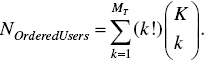
It will be very difficult to perform this ESS DPC for a practical MU‐MIMO BC. The total number of searches required for DPC as computed by 5.1 will be very high, which will not be feasible for real‐time communications where the scheduling interval is a few milliseconds. To fill this gap, the authors in [13] have implemented an evolutionary algorithm (Binary Genetic Algorithm [BGA]) to search the set of best users/antennas, which will result in the maximum system sum‐rate well within the span of the scheduling interval. This is explained in Section 5.2. The authors in [11, 12] have used GA for cross‐layer scheduling of MU‐MIMO systems with single and multiple carriers, respectively. Elitism and adaptive mutation (AM) has been proposed to be a preferred mutation process for GA as discussed by [11, 24]. The authors of [13] have been motivated by the aforementioned works to develop a combined user and antenna scheduling (CUAS) scheme for single carrier MU‐MIMO broadcast systems using BGA with elitism and AM. Moreover, they considered random beamforming [19, 23]. In [13], it has been shown that using BGA with elitism and AM for CUAS achieves the same system sum‐rate as that of ESS with much less computation overhead. Moreover, CUAS using BGA with elitism and AM attains higher system sum‐rate than some of the classical sub‐optimal limited feedback scheduling schemes [23] for MU‐MIMO downlink systems.

The importance of CSI at the transmitter (CSIT) has been discussed widely and exhaustively in the literature for multi‐antenna systems [17–19, 23,25–27]. The CSIT helps the transmitter for beamforming/precoding to transmit the message symbols to the appropriate antenna at UE from each of the antennas at the transmitter. This practice helps in achieving the maximum system sum‐rate for the broadcasting scenario of MU‐MIMO. However, it has also been discussed that to send the CSI from each UE to the transmitter, an uplink channel is utilized. This reduces the spectrum efficiency of the data communications by consuming the probable useful bandwidth for carrying the CSI. Moreover, this phase of communication introduces delay into the system, which should be minimized. Therefore, limited feedback scheduling schemes have been proposed and discussed [16, 17, 19, 23,28–35], where the main motive of the research is to reduce the feedback data volume from UE to the BS. Signal‐to‐interference‐plus‐noise ratio (SINR) has been considered as a suitable form of CSI to be fed back from UE to the BS. The authors in [23] discussed the quantization of SINR with one‐bit and a fixed quantization threshold, which will reduce the feedback overhead. It has been shown that this technique of one‐bit SINR quantization fails to exploit the concept of MUD. Furthermore, this scheme attains less system sum‐rate compared to scheduling schemes with the full feedback of CSI.

Therefore, to mitigate the limitations pertaining to one‐bit quantization process, the authors in [17] studied the effect of multi‐bit SINR quantization to achieve system sum‐rate close to that of full feedback scheduling scheme with not so much feedback overhead as the full feedback of CSI from UEs to the BS. For multi‐bit quantization, the selection of optimal quantization thresholds is very important to get the benefit of using the multi‐bit quantization process. Therefore, optimal quantization threshold selection is necessary. The system sum‐rate of the MU‐MIMO BC is a function of scheduled users' SINR value, number of transmit antennas (M_T ), best receive antenna of the scheduled users for corresponding transmit antenna, and number of users (K). Moreover, it has been shown that the system sum‐rate is a function of number of users (K) and quantization threshold (Ξ) for a given set of M_T, N_R, and the received signal‐to‐noise ratio (SNR) (Ξ), i.e. C_{sum − rate} = f(K, Ψ), where C_{sum − rate} is the achievable system sum‐rate. For finding the optimal quantization threshold, a solution to = 0 has to be obtained. However, it has also been discussed in [23] that a closed‐form solution to = 0 is not tractable. Due to this multi‐variable relation, deriving closed‐form solution of the optimal quantization thresholds (Ξ) is very much more complex for MU‐MIMO systems. Moreover, the range over which the optimal quantization thresholds (Ξ) can acquire value is very wide. For this reason, the exhaustive search over this wide range of values is required for efficient user/antenna scheduling process for multi‐antenna systems. To address these difficulties, GA has been used to select the optimal quantization thresholds (Ξ) for obtaining the highest system sum‐rate. From a system implementation point of view, the optimal quantization thresholds have been expressed in terms of system SNR value and number of antennas at the transmitter.

It has been shown in [17] that quantization with four bits along with optimum quantization thresholds is sufficient to achieve system throughput close to that of full feedback scheduling [23]. The authors in [17] have discussed two user/antenna scheduling schemes based on four‐bit quantization of SINR. In the first scheme, all UEs send the four quantized bits representing the highest SINR among all M_T N_R SINR values and the corresponding transmit antenna index to the BS for scheduling purposes. However, this scheme has the limitation of assigning a particular receive antenna of a UE to multiple transmit antennas and keeping some of the antennas at the BS idle by not sending any message signal from them. Therefore, the second scheme, named the optimistic scheme, has been proposed where these two aforementioned limitations are addressed properly. The methodology of GA has been adopted to find the optimal quantization threshold values for both of these scheduling schemes. Furthermore, for attaining the least feedback overhead of CSI a four‐bit quantization process has been proposed in the literature. This scheme of four‐bit quantization is also successful in providing a resulting system throughput very close to the optimum values. It is well known that the quantization threshold plays an absolutely vital role in the multi‐bit quantization process. However, selection of the optimum quantization thresholds is also cumbersome. Hence GA is proposed to find the optimum quantization threshold values for MU‐MIMO systems. This process is explained in detail in Section 5.3.

The advantages of the MU‐MIMO system have been discussed earlier in this chapter. The requirement for wide‐band communication channels increases due to the huge increase of users' data traffic. These wide‐band communication channels are more frequency‐selective in nature [36, 37]. To overcome the limitations of these wide‐band frequency selective channels, the orthogonal‐frequency‐division‐multiplexing (OFDM) technique has been used widely. OFDM converts the wide‐band frequency‐selective channel into multiple narrow‐band frequency‐flat fading sub‐channels, which can be modulated independently [38]. This robustness of OFDM makes it a suitable candidate for the underlying technology of enhanced data rate communication framework. Therefore, MIMO and OFDM are integrated together (MIMO‐OFDM) to be the backbone of current and future wireless technologies [39].

The limitations associated with feedback data from UEs to the BS have been discussed in detail previously in this section. The feedback load burden increases with number of users, number of antennas at the transmitter, and number of sub‐carriers for the MU MIMO‐OFDM system. The MU MIMO‐OFDM system has a detrimental effect on the system by increasing the feedback overload by many fold. Design and development of limited feedback user/antenna scheduling schemes becomes very important for MU MIMO‐OFDM systems. The computational complexity increases further for MIMO‐OFDM systems as MIMO‐OFDM systems have multiple carriers. The scheduling process explained for MU‐MIMO systems needs to be implemented for all the sub‐carriers present in a MU MIMO‐OFDM system. Quantization of real‐time SINR values has also been shown to be a promising technique for reducing the feedback burden for MU MIMO‐OFDM systems [25]. The authors in [25] have shown that quantization of SINR with four‐bits is sufficient to have achievable system sum‐rate close to the optimal with the least feedback overhead. As discussed previously in this chapter, finding the optimal quantization threshold values for MU MIMO‐OFDM systems is absolutely vital from a system design point of view. Moreover, the range of the possible values for the quantization threshold is very wide for MIMO‐OFDM systems. Therefore, to facilitate the process of finding optimal quantization threshold values the technique of GA has been used to find the optimal values swiftly [25]. This is explained in detail in Section 5.4.

The quantization process helps in achieving reduction of feedback overhead. However, in the MU MIMO‐OFDM system, clustering of adjacent sub‐carriers has to be carried out to attain a further reduction of feedback load. Therefore, each UE finds the highest SINR value corresponding to each transmit antenna and adds them for a cluster of sub‐carriers. Then each UE sends the four‐bit quantized bits representing the added value to the BS, which employs both the techniques of clustering and quantization with four‐bits. The importance of selecting proper quantization threshold has been discussed earlier in this section. Therefore, to find optimal quantization thresholds for a different MU MIMO‐OFDM system is absolutely crucial to attain reduction of the feedback overhead. Moreover, it has been shown that the system sum‐rate is a function of the number of users (K) and quantization threshold (Ψ) for a given set of M_T, N_R, the received SNR (Ξ), and cluster size (L_C ), i.e. C_{sum − rate} = f(K, Ψ), where C_{sum − rate} is the achievable system sum‐rate. To find the optimal quantization threshold, a solution to = 0 has to be obtained. However, it has also been discussed in [23] that a closed‐form solution to = 0 is not tractable. Moreover, the search space for the quantization thresholds for MU MIMO‐OFDM is large. Therefore, authors in [25] have used BGA for finding the optimal four‐bit quantization threshold values, which is discussed in Section 5.4.

Also, the real‐time joint selection of a transmit and receive antenna pair in MIMO systems involves high computational complexity. This complexity increases with the number of transmit and receive antennas. Hence, Binary Particle Swarm Optimization (BPSO) is used for a low complex solution to this problem. Moreover, it is shown that convergence rate is reduced by applying cyclically shifted initial population. MIMO systems have offered a lot of benefits but also incur higher hardware cost by using a multiple radio frequency (RF) chain, which includes power amplifier, analog‐to‐digital converters, etc. This hardware cost can be brought down by using a subset of these antennas, which have good channel conditions [40]. Therefore, users in [41] have studied joint transmit and receive antenna selection (JTRAS) for single‐user MIMO systems. The exhaustive search scheme for this is computationally inefficient. The system parameters used in this chapter till now hold true for this subsection as well. The MIMO system has a transmitter with M_T transmit antennas and a receiver with N_R receive antennas. It has been further assumed that the transmitter has M_t and the receiver has N_r number of RF chains available to them. Here, the transmitter has been assumed to have no information about the channel and the receiver has the CSI. The receiver performs the selection of both N_r and M_t number of receive and transmit antennas. The MIMO system considered here is closed‐loop MIMO channel, where the receiver sends the information about the selected transmit antennas to the transmitter.

The number of possible ways of joint selection of transmit and receive antenna is given as

(5.2)

This value grows with the number of transmit and receive antennas. The channel capacity associated with each of these combinations has been expressed as:

(5.3)

where I_a is the a × a identity matrix, H_i is the channel between the receive and transmit antenna associated with ith combination and (A)^* is the complex conjugate transpose of a matrix (A). The utility function or the cost function for this problem has been assumed to be 5.3. However, evaluation of 5.3 for N_ESS number of combinations of transmit and receive antennas could not be accomplished during a packet time which is of the order of a few milliseconds. To overcome this, a low computationally burdened joint transmit and receive antenna selection scheme employing BPSO has been suggested and discussed in [41]. This process is being elaborately presented in Section 5.5.1.

Further, the usage of BPSO will be shown for a MU‐MIMO system, where the joint user scheduling and receive antenna selection (JUSRAS) will be performed by BPSO as proposed and described in [42]. The computational complexity of JUSRAS increases with number of users in the system K and number of receive antennas at each UE (N_R ). As a consequence, BPSO has been used for JUSRAS as explained in Section 5.5.2. Moreover, authors in [43] have proposed a hybrid discrete particle swarm optimization (DPSO) algorithm with Levy flight for scheduling MIMO radar tasks. An efficient scheduling scheme using GA has been proposed by the authors in [44] for massive MIMO systems. In this paper, it has been shown that the achievable system throughput by this scheduling scheme using GA is almost the same as that of an exhaustive search scheduler with extensively less implementation complexity.

5.2 CUAS Scheme Using GA

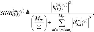
A closed loop MU‐MIMO broadcasting system has been considered in [13], where each UE sends its CSI in the form of SINR to the BS for scheduling/selection of best channel conditioned UEs for data transmission. The instantaneous SINR at the n_r th antenna of the kth UE considering the data transmitted from m_t transmit antenna as the required signal is expressed as

(5.4)

where h_k (n_r, m_t) is the channel element between the n_r antenna of the kth UE and the m_t antenna of the BS, Ξ_k is the received SNR of the kth UE. This is independent and identically distributed (i.i.d) complex Gaussian channel gain coefficient with zero mean and unit variance, i.e. . The total transmit power by all the antennas at the BS is assumed to be unity. The achievable sum‐rate of the MU‐MIMO system is expressed as

(5.5)

The possible number of ways of scheduling M_T number of users from all K users according to DPC is given in Eq. (5.1), which is very high for a higher number of users. To have a subset of this large set, the authors in [13] removed some of the possible user combinations by considering such constraints as:

1. User combinations having same M_T users will be evaluated only once.
2. No user should be served by more than one transmit antenna.
3. User combinations having duplicate users should be removed.

By considering these constraints, the total number of user combinations evaluated by the CUAS is given by

(5.6)

This number also grows very fast with a higher number of transmit antennas and users. Because of this, the number of evaluation of the utility function is very high. This much computation cannot be done within the time frame of current high‐speed communication systems. Therefore, BGA with elitism and AM has been used for the CUAS by the authors of [13] to reduce the computational complexity, so as to complete the scheduling process well within the stipulated time frame. Moreover, to facilitate this process, high‐end digital signal processing (DSP) units are used at the BS.

5.2.1 GA Methodology Followed for CUAS

Evolutionary algorithms were considered by Holland [45] in 1975, which mimic the biological system's evolution process. GA delivers solutions close to the optimal ones swiftly with less computational complexity. Solutions to non‐convex optimization utility functions can also be delivered by GA. BGA has been considered for solving the discussed user/antenna scheduling scenario for the MU‐MIMO broadcast network due to the features of GA highlighted above. In this section, BGA has been chosen to be used. Therefore, the chromosomes will have a string of combination of bit “0” and bit “1.”

The set of constraints below have been considered by the authors in [13] for obtaining near‐optimal scheduling solution incurring less computational complexity:

1. Each antenna at BS should send independent messages to unique UEs. Therefore, no rows in the population should contain a duplicate UE's index.
2. Unique population should be considered, i.e. all the UE indices in every row should be unique.
3. The UE index has been constrained to acquire any value ranging from 1 to K. It should not go beyond this interval.

During the process of population initialization, these three constraints need to be checked. Initialization of the population should be continuously repeated till none of these three constraints violate. In each generation, the fitness value of each chromosome has to be evaluated and then sorted in descending order. The probability of crossover has been assumed to be unity. After getting the children from the crossover process, a process of mutation has been carried out on the newly formed children by flipping any gene randomly. Adaptive mutation has been considered by the authors of [13], where the probability of mutation was continuously evaluated rather than keeping it constant. According to AM, the mutation probability changes according to the mean and standard deviation of the present population, according to the relation mentioned below:

(5.7)

where σ_P, μ_P are the standard deviation and mean of the present population's fitness value, β₁ = 1.2 and β₂ = 10 (adopted from [11]). For comparison purposes, the authors assumed P_m to be 0.1 when simple mutation is considered. The aforementioned three constraints need to be satisfied by the children formed after mutation. If any constraints get violated, then randomly some genes are flipped till no constraints are violated. Moreover, elitism has also been adopted in the BGA, where the best chromosomes of the present generation are passed on to the next generation. Better children get produced by this process. The crossover and mutation process has been depicted in Figure 5.1. This BGA process is explained in Figure 5.2.

5.2.2 Simulation Results and Discussion

Different performances of the discussed BGA have been demonstrated to emphasize the benefits obtained as compared to various other schemes. The number of antennas at each UE is assumed to be two. The number of generations assumed for BGA is 25. In Figure 5.3, the system sum‐rate obtained by this BGA process with AM and elitism has been compared with a limited feedback scheduling scheme of [23], ESS, and BGA process with normal mutation (with P_m to be 0.1). Each point in these figures is the averaged value of 100 independent simulations. From these figures, it has been observed that BGA with elitism and AM succeed in achieving system sum‐rate close to that of ESS (DPC scheme). It has also been shown that the BGA process discussed with AM and elitism attains a higher system sum‐rate than that of the limited feedback scheduling scheme discussed in [23].

The authors of [13] have also discussed a parameter called the percentage deviation from optimal (PDFO) as defined below:

(5.8)

where θ can be the BGA process with and without AM and elitism, limited feedback scheduling scheme of [23]. This parameter gives an idea about the extent by which the system sum‐rate attained by the methods other than ESS (DPC scheme) differ from the system sum‐rate obtained by ESS (DPC scheme). In Figure 5.4, the PDFO for the above scenarios is presented. Each point in these figures is the averaged value of 100 independent simulations. The number of generations considered is 25 for all these figures. In [13], the authors have also shown the generation‐wise performance of the proposed BGA with and without elitism and AM. The system sum‐rate obtained by the proposed BGA with and without elitism and AM has been plotted with respect to number of generations in Figure 5.5. It has been observed that the system sum‐rate attained at a particular generation is always more than that of the previous generation. This shows the correctness of the BGA implementation. The mutation probability (P_m) for the normal mutation is assumed to be 0.1. Here also, each point in these figures is the averaged value of 100 independent simulations.

The stochastic behavior of the proposed BGA has been shown in [13]. The empirical distribution for the histogram of the attained sum‐rate by the proposed BGA with and without AM and elitism is showcased in Figure 5.6.

Each point in these figures is the averaged value of 1000 independent simulations. The system sum‐rate (expressed in bps/Hz) is presented in the horizontal axis and the total number of incidences during 1000 independent simulations are presented in the vertical axis of these histograms. It has been observed that the interval of sum‐rate achieved by the BGA with elitism and AM is higher than the BGA without elitism and AM. Moreover, the occurrences of higher system sum‐rate are also more for the BGA with elitism and AM than the BGA without elitism and AM. These are the explanations for achieving higher system sum‐rate by the proposed BGA.

5.2.3 Computational Complexity for CUAS Scheme

It is essential to demonstrate the computational complexity analysis of the proposed BGA mechanism in [13]. The authors in [13], have represented the computational complexity in terms of the number of complex multiplications and additions (CMAs) as shown in [41, 42]. There can be a total M_T N_R number of SINRs per UE. For calculation of each SINR, 2M_T CMAs are required as per Eq. (5.4). Therefore, altogether CMAs will be computed for Eq. (5.5). The total number of CMA computations required for ESS (DPC) is:

(5.9)

The total number of CMA computations required for the BGA with elitism and AM is:

(5.10)

where P is the population size, P_c is the crossover probability, and N_g is the number of generations required for the BGA. In [13], the authors show the time complexity of ESS (DPC) and the proposed BGA technique by considering high computational DSP processors like the multi‐core ARM and DSP processor 66AK2Ex series of Texas Instruments (this processor can perform up to 44.8 Giga multiply‐accumulate per second) for different MU‐MIMO configurations. It has also been shown that the implementation of the BGA with elitism and AM is very much possible within the time duration of packet data communications, which is in the range of a few milliseconds [11, 12, 46].

In Table 5.1, the time complexity required by ESS (DPC) and the BGA scheme with AM and elitism has been shown for some MU‐MIMO scenarios. Here, the number of CMA computations are tabulated along with the estimated execution time, taking into account the Texas Instruments DSP processor series 66AK2Ex for computation.

System Parameters
{MT, NR, K, P, Ng }	ESS (DPC)		BGA
	CMAs	Time (ms)	CMAs	Time (ms)
5, 3, 25, 25, 10	39 847 500	0.88945	562 500	0.012556
7, 3, 30, 30, 15	4.1897e+09	93.5	2 778 300	0.062016
8, 2, 20, 20, 20	257 986 560	5.8	2 457 600	0.054857

5.3 Selection of Optimum Quantization Thresholds for MU‐MIMO Systems Using GA

The importance of selecting the optimal quantization thresholds for multi‐bit quantization process has been discussed in Section 5.2. Here, SINR quantization with four bits is considered for MU‐MIMO systems. The four bits representing a floating point SINR value are defined as below:

where Ψ is the highest quantization threshold. For different quantization thresholds (from Ψ₁ to Ψ₁5), it has been assumed that

1. Ψ₀ = 0
2. Ψ₁₅ = Ψ
3. Ψ₁₆ = ∞
4. the separation between two successive quantization levels is given by .

5.3.2 Simulation Results and Discussion

Here, a heterogeneous MU‐MIMO broadcasting system has been considered for finding the optimal quantization threshold values. In this system, it has been assumed that all the users present in a cellular area of a BS do not enjoy the same received SNR. This is due to different path losses and the shadowing effect at various positions with respect to the transmitter. In this model, for simplicity it has been assumed that all the users K have been divided into Z number of user groups. Each user group has same number of users, i.e. K/Z.

The instantaneous SINR for this system has been given as below:

(5.11)

where represents the average received SNR of user k belonging to the user group z. The achievable average sum‐rate of the system can be computed as:

(5.12)

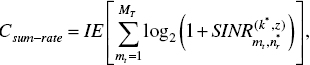
where IE[.] is the expectation operator and is the SINR value achieved by the scheduled user k ^* among the users who have sent the highest decimal value of the four‐bit SINR quantized feedback corresponding to the m_t antenna at the BS. This scheduled user is assumed to the present in the zth user group according to the received SNR value. The optimum quantization threshold values required by the four‐bit quantized feedback scheduling scheme and four‐bit quantized optimistic scheduling scheme for various MU‐MIMO systems have been computed by the process discussed above using BGA. These optimum quantization threshold values are tabulated in Table 5.2.

It has been observed from Figures 5.7 and 5.8 that the system sum‐rate achieved by these two schemes employing four‐bit SINR quantization is close to that of the full feedback scheduling scheme of [23] and the limited feedback scheduling scheme of [18]. Moreover, the feedback overhead of these two scheduling schemes employing four‐bit SINR quantization is less than that of full feedback scheduling scheme of [23] and the limited feedback scheduling scheme of [18].

Received SNR Ξ	Number of antennas at the BS (MT )	Ψ15 for four‐bit quantized feedback scheduling scheme as a multiple of received SNR	Ψ15 for four‐bit quantized optimistic feedback scheduling scheme as a multiple of received SNR
5 dB	2	3	2.5
	3	2	2
	4	1	1
	5	1	1
10 dB	2	2	2
	3	1	0.9
	4	0.6	0.6
	5	0.5	0.4

5.4 Selection of Optimum Quantization Thresholds for MU MIMO‐OFDM Systems Using GA

The previous system parameters used in Sections 5.2 and 5.3 are valid with the introduction of some more system parameters like number of sub‐carriers (L) and cluster size (L_C ). The channel matrix between user k over sub‐carrier l can be formulated as [36, 47]:

(5.13)

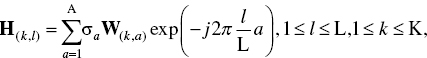
where the exponential function is denoted by exp(.). The power delay profile (PDP) of the MIMO‐OFDM broadcast network is expressed as [47]:

(5.14)

The values of A and D_exp have been assumed to be 8 and 2 respectively as [36, 47]. These PDPs are normalized as

(5.15)

The instantaneous SINR of user k over lth sub‐carrier is given as:

(5.16)

The achievable system sum‐rate of this broadcast system can be computed as:

(5.17)

where is the sum‐rate of subcarrier l, which is expressed as

(5.18)

5.4.1 GA Methodology Followed to Find the Optimal Ψ for MU MIMO‐OFDM

The BGA process is described below. A small change in quantization threshold will have greater impact on the achievable system sum‐rate due to the process of clustering of adjacent sub‐carriers. To address this, the process of elitism and AM has been followed with a very narrow increment in the successive probable quantization threshold values. The utility function is Eq. (5.17). The minimum and maximum probable values for the quantization threshold are 0.1 and 100 respectively. Moreover, two successive probable quantization threshold values are separated by 0.1. The number of binary genes in each chromosome has been assumed to be . The probability of crossover (P_c) has also been fixed at 0.8. The mutation probability for AM has been computed as per Eq. (5.7). The probability of breeding of any chromosome j from a population of size P_g has been computed as:

(5.19)

The process of BGA needs to be followed for Ng number of generations.

The constraints mentioned below need to be checked for every chromosome of population for each generation:

1. No chromosome should be allowed with all its genes as bit “0.”
2. No chromosome should be allowed to have a decimal value greater than 1000.
3. No two chromosomes of any population should have duplicate values.

For any generation g, the fitness value of each chromosome (including the parents and children resulted from crossover and mutation) of the population is computed and they are sorted in the descending order. Then, the first P_g number of chromosomes are allowed to move to the next generation, according to elitism. This BGA process is explained in Figure 5.2.

5.4.3 Achievement of Reduction in Computational Complexity by BGA

It has been shown in [25] that reduction in computational complexity has been achieved by implementing the BGA discussed above for MU MIMO‐OFDM broadcasting network. The total number of times the utility function gets executed for the ESS process and the BGA process are given by N_ESS and N_BGA respectively. N_ESS = 100/0.1 = 1000, which includes all the possible options for quantization threshold as 0.1, 0.2, …, 100. The expression for N_BGA has been given as the expression below:

	Ξ = 5 dB		Ξ = 10 dB
MT = NR	LC = 16	LC = 32	LC = 16	LC = 32
2	45	75	35	60
3	25	65	20	30
4	20	35	10	20
5	15	25	10	15

(5.20)

By using P_g = 10, P_c = 0.8, and N_g = 3, N_BGA is computed to be 78. Therefore, the reduction in computation complexity achieved by the BGA is .

5.5 Scheduling for MIMO Systems Using PSO

In recent years, PSO has also been used for these kinds of user/antenna scheduling schemes [41, 42]. Authors in [41, 42] have used the BPSO technique for joint transmit and receive antenna selection for single‐user MIMO systems and joint user and receive antenna selection for multi‐user MIMO systems respectively. It has been shown in these papers that low computational complexity solutions to scheduling problems have been achieved by using BPSO. Moreover, the authors of [41, 42] have presented that using a particular technique of BPSO which uses cyclically shifted initial population achieves an earlier convergence than the conventional BPSO method.

5.5.1 JTRAS in Single‐User MIMO Systems Using BPSO

In this section, the use of BPSO will be shown for JTRAS in single‐user MIMO systems. The social behavior of fish schooling and bird flocking has given rise to PSO. PSO has been proved to be a robust optimization approach which can find the global optimum very swiftly [48]. PSO is an population‐based evolutionary algorithm, which consists of particles as individuals and the collection of particles is called a swarm or population. In this process, particles move in a N‐dimensional space, where N is the number of variables present in the cost function. Particles change their position to find the optimal solution based on their own and other particles’ experience. In BPSO [49], the position of each particle is represented as a string of binary bits of “0” and “1.”

The variables and notations used in [41] are as below:

• The search space consisting of all possible solutions, which is denoted as the combinations presented in N_ESS .
• The fitness or cost function which is denoted as Eq. (5.3).
• The size of population (or swarm) (P).
• Number of iterations (N_g ).
• Dimension of the particle position (i.e. the number of variables in the cost function).
• Two parameters c₁ and c₂ are used for social and cognitive control respectively over the movement of the particle. It has been assumed that c₁ = c₂ = 2.
• In conventional BPSO, the initial population is assumed to be selected randomly. However, in this paper, authors have used an initial feed as the initial population to reduce the convergence time. Then some cyclic shift of this inital feed is also considered for some of the particles in the initial swarm.
• A cyclically shifted initial swarm also does not allow biasing to the initial population.

5.5.1.1 Simulation Results and Discussion

The 10% outage capacity for a MIMO system has been presented in Figure 5.11 by considering the system parameters as those of [41]. For this figure, the system parameter values are M_T = 6, N_R = 30, M_t = 3, N_r = 3, N_g = 25, P = 25, c₁ = 2, c₂ = 2. The GA used is priority‐based GA, as discussed in [50].

The performance of this BPSO technique has been shown in Figure 5.12 with respect to number of iterations. The convergence of this BPSO technique with a cyclic shift of initial feed performs better than GA and BPSO with random initialized population. The MIMO system parameters considered for Figure 5.12 are M_T = 8, N_R = 12, M_t = 2, N_r = 5, N_g = 10, P = 25, c₁ = 2, c₂ = 2, Ξ = 25 dB.

It can be observed that BPSO performs better than GA for this JTRAS.

5.5.2 JUSRAS in MU‐MIMO Systems Using BPSO

Here a multi‐user MIMO system is considered. The parameters used earlier will remain valid for this section as well. There are K number of UEs, where each UE has N_R number of antennas. The BS has M_T number of antennas. In this section, the usage of BPSO for JTRAS in single‐user MIMO systems will be shown. The authors in [42] have considered the uplink channel for this JUSRAS problem. The total power at the BS has been divided between all the UEs equally, i.e. each UE has amount of power, where T is the total power present at the BS. Then, each of the antennas at UE also has the same power, i.e. . Further, it has also been assumed that the UEs do not have the uplink CSI whereas the BS has the complete uplink CSI. The instantaneous channel sum‐rate can be expressed as 5.3. This is also the utility function for the JUSRAS.

For the JUSRAS, the total number of potential joint user and receive antenna selections are given as:

(5.21)

where K_s is the total number of users selected. The number of probable candidates (N_ESS) increases with number of users and number of antennas. These many candidates cannot be examined within the period of a symbol duration of the current high data rate communication systems. Therefore, the authors of [42] have proposed to use BPSO to have a better solution. The BPSO technique with cyclically shifted population has been used for the JUSRAS as that was used for the JTRAS in Section 5.5.1.

5.5.2.1 Simulation Results and Discussion

In this section, the performance of this BPSO method with a cyclic shifted population has been analyzed by three ways of finding the PDFO, system sum‐rate per generation, and the standard deviation achieved. The GA technique, which has been used here for comparison purposes, is the basic GA method where probability of crossover and mutation have been assumed to be 0.9 and 0.1 respectively. The PDFO has been defined as:

(5.22)

where is the sum‐rate achieved by the exhaustive search technique, which yields the maximum system sum‐rate and technique can be either BPSO or GA.

The MU‐MIMO system parameters considered for Figure 5.13 are N_R = 2, M_t = 2, M_T = 10, K_s = 4, and K = 12. It has been clearly observed that the PDFO for GA is more than BPSO, which underlines that the system sum‐rate achieved by BPSO is more than GA for this JUSRAS.

The MU‐MIMO system parameters considered for Figure 5.14 are N_R = 2, M_t = 4, M_T = 8, K_s = 3, K = 10, and Ξ = 20 dB. The population size used for BPSO and GA for this figure has been assumed to be 10, which is equal to the number of total users in this uplink scenario.

The MU‐MIMO system parameters considered for Figure 5.15 are N_R = 2, M_t = 2, M_T = 8, K_s = 4, and K = 14. Here also, the population size for BPSO and GA has been assumed to be 14, which is the number of users present in the MU‐MIMO system. The standard deviation achieved by the BPSO is less than that of the GA, which emphasizes that BPSO attains better system sum‐rate than the GA technique.

5.6 Conclusion

The use of GA and PSO for user and antenna scheduling of multi‐user multiple antenna systems has been discussed in this chapter. The search space for both user and antenna scheduling process is large and this space grows dramatically with the increase in numbers of users and antennas at both transmitter and receiver. The use of GA has resulted in a convincing reduction in the magnitude of such a problem. It has been demonstrated that a reduction in computational complexity has been achieved by using BGA for the MU‐MIMO broadcast network. The estimated timing for completion of the scheduling process by BGA with elitism and AM has been shown to be well within the required duration of the current and next generation packet data communications. Moreover, the advantage of using elitism and AM in achieving higher system sum‐rate than the limited feedback scheduling scheme has also been shown. The PDFO achieved by BGA elitism and AM is less than that of limited feedback scheduling and BGA without elitism and AM. Quantization of CSI by multiple bits has been proposed and discussed for achievement of feedback overhead reduction of the closed‐loop MU‐MIMO systems. However, multi‐bit quantization is effective only when the optimal quantization thresholds are selected. The search space for this optimal quantization threshold is very large. Therefore, BGA has been used for finding the optimal quantization thresholds for both MU‐MIMO and MU‐MIMO‐OFDM systems. Further, these quantization thresholds have been expressed in terms of system SNR (Ξ) for easier system implementation. Both homogeneous and heterogeneous MIMO systems have been considered. The use of PSO has also been discussed for JTRAS in single‐user MIMO systems and JUSRAS for MU‐MIMO systems. The performance of PSO with a cyclic shifted initial population after each generation has been shown to be better than GA and basic PSO. It has also been shown that this kind of PSO outperforms GA in terms of the achievable system sum‐rate. The standard deviation achieved by PSO for JTRAS and JUSRAS is less than that of GA.

References

1. 1 Knopp, R. and Humblet, P.A. (1995). Information capacity and power control in single cell multiuser communications. Proceedings of the IEEE Int. Conf. Commun. (June 1995), 331–335.
2. 2 Letaief, K.B. and Zhang, Y. (2006). Dynamic multiuser resource allocation and adaptation for wireless systems. IEEE Wirel. Commun. Mag. 13: 38–47.
3. 3 Costa, M.H.M. (1983). Writing on dirty paper. IEEE Trans. Inf. Theory 29: 439–441.
4. 4 Caire, G. and Shamai, S. (2003). On the achievable throughput of a multiantenna gaussian broadcast channel. IEEE Trans. Inf. Theory 43: 1691–1706.
5. 5 Mazzarese, D.J. and Krzymien, W.A. (2007). Scheduling algorithms and throughput maximization for the downlink of packet‐data cellular systems with multiple antennas at the base station. IEEE Trans. Veh. Technol. 43: 215–260.
6. 6 Ajib, W. and Haccoun, D. (2005). An overview of scheduling algorithms in MIMO‐based fourth‐generation wireless systems. IEEE Net. 19 (5): 43–48.
7. 7 Chung, J., Hwang, C.S., Kim, K., and Kim, Y.K. (2003). A random beamforming techniques in MIMO systems exploiting multiuser diversity. IEEE J. Sel. Areas Commun. 21: 848–855.
8. 8 Gozali, R., Buehrer, R.M., and Woerner, B.D. (2003). The impact of multiuser diversity on space‐time block coding. IEEE Commun. Lett. 7: 213–215.
9. 9Hochwald, B.M., Marzetta, T.L., and Tarokh, V. (2004). Multiple‐antenna channel hardening and its implications for rate feedback and scheduling. IEEE Trans. Inf. Theory 50: 1893–1909.
10. 10 Sharma, N. and Ozarow, L.H. (2005). A study of opportunism for multipleantenna systems. IEEE Trans. Inf. Theory 51: 1804–1814.
11. 11 Elliott, R.C. and Krzymien, W.A. (2009). Downlink scheduling via genetic algorithms for multiuser single‐carrier and multicarrier MIMO systems with dirty paper coding. IEEE Trans. Veh. Technol. 58: 3247–3262.
12. 12 Lau, V.K.N. (2005). Optimal downlink space‐time scheduling design with convex utility functionsmultiple‐antenna systems with orthogonal spatial multiplexing. IEEE Trans. Veh. Technol. 54: 1322–1333.
13. 13 Pattanayak, P. and Kumar, P. (2015). A computationally efficient genetic algorithm for MIMO broadcast scheduling. Elsevier Appl. Soft Comput. 37: 545–553.
14. 14 Bayesteh, A. and Khandani, A. (2005). On the user selection for MIMO broadcast channels. Proceedings of the IEEE Int. Symp. Inf. Theory, Adelaide, Australia (4–9 September), 2325–2329.
15. 15 Jaewoo, S. and Cioffi, J.M. (2009). Multiuser diversity in a MIMO system with opportunistic feedback. IEEE Trans. Veh. Technol. 58: 4909–4918.
16. 16 Min, M., Kim, D., Kim, H., and Im, G. (2013). Opportunistic two‐stage feedback and scheduling for MIMO downlink systems. IEEE Trans. Commun. 61: 312–324.
17. 17 Pattanayak, P. and Kumar, P. (2016). Quantized feedback MIMO scheduling for heterogeneous broadcast networks. Wirel. Netw. 23: 1449–1466.
18. 18 Pattanayak, P., Roy, K.M., and Kumar, P. (2015). Analysis of a new MIMO broadcast channel limited feedback scheduling algorithm with user grouping. Springer Wirel. Pers. Commun. 80: 1079–1094.
19. 19 Sharif, M. and Hassibi, B. (2005). On the capacity of MIMO broadcast channels with partial side information. IEEE Trans. Inf. Theory 51: 506–522.
20. 20 Swannack, C., Uysal‐Biyikoglu, E., and Wornell, G.W. (2005). MIMO broadcast scheduling with limited channel state information. Proc. Annual Allerton Conf. on Commun., Control and Computing, September.
21. 21 Wunder, G., Schreck, J., and Jung, P. (2012). Nearly doubling the throughput of multiuser MIMO systems using codebook tailored limited feedback protocol. IEEE Trans. Wirel. Commun. 11: 3921–3931.
22. 22 Yoo, T. and Goldsmith, A. (2006). On the optimality of multiantenna broadcast scheduling using zero‐forcing beamforming. IEEE J. Select. Areas Commun. 24: 528–541.
23. 23 Zhang, W. and Letaief, K.B. (2007). MIMO broadcast scheduling with limited feedback. IEEE J. Select. Areas Commun. 25: 1457–1467.
24. 24 Yang, C., Han, J., Li, Y., and Xu, X. (2013). Self‐adaptive genetic algorithm based MU‐MIMO scheduling scheme. Proc. IEEE International Conf. on Commun. Technol.: 180–185.
25. 25Pattanayak, P. and Kumar, P. (2017). Quantized feedback scheduling for MIMO‐OFDM broadcast networks with subcarrier clustering. Elsevier Ad Hoc Netw. 65: 26–37.
26. 26 Pattanayak, P. and Kumar, P. (Apr 2018). Combined user and antenna scheduling scheme for MIMO–OFDM networks. Telecom Systems: Modelling, Analysis, Design and Management 70: 3–12. https://doi.org/10.1007/s11235‐018‐0462‐0.
27. 27 Pattanayak, P. and Kumar, P. (2019). An efficient scheduling scheme for mimo‐ofdm broadcast networks. AEU Int. J. Electron. Commun. 101: 15–26. https://doi.org/10.1016/j.aeue.2019.01.017.
28. 28 Al‐Saedy, M., Al‐Imari, M., Al‐Shuraifi, M., and Al‐Raweshidy, H. (2017). Joint user selection and multimode scheduling in multicell MIMO cellular networks. IEEE Trans. Veh. Technol. 66 (12): 10962–10972. https://doi.org/10.1109/TVT.2017.2717909.
29. 29 Fang, F., Zhang, H., Cheng, J. et al. (2017). Joint user scheduling and power allocation optimization for energy‐efficient NOMA systems with imperfect CSI. IEEE J. Sel. Areas Commun. 35 (12): 2874–2885. https://doi.org/10.1109/JSAC.2017.2777672.
30. 30 Femenias, G. and Riera‐Palou, F. (2016). Scheduling and resource allocation in downlink multiuser MIMO‐OFDMA systems. IEEE Trans. Commun. 64 (5): 2019–2034. https://doi.org/10.1109/TCOMM.2016.2547424.
31. 31 Hou, J., Yi, N., and Ma, Y. (2015). Joint spacefrequency user scheduling for MIMO random beamforming with limited feedback. IEEE Trans. Commun. 63 (6): 2224–2236. https://doi.org/10.1109/TCOMM.2015.2432772.
32. 32 Liu, H., Gao, H., Yang, S., and Lv, T. (2017). Low‐complexity downlink user selection for massive MIMO systems. IEEE Syst. J. 11 (2): 1072–1083. https://doi.org/10.1109/JSYST.2015.2422475.
33. 33 Ronasi, K., Niu, B., Wong, V.W.S. et al. (2014). Throughput‐efficient scheduling and interference alignment for MIMO wireless systems. IEEE Trans. Wirel. Commun. 13 (4): 1779–1789. https://doi.org/10.1109/TWC.2014.031314.122040.
34. 34 Wang, H., Wang, W., Lau, V.K.N., and Zhang, Z. (2017). Hybrid limited feedback in 5G cellular systems with massive MIMO. IEEE Syst. J. 11 (1): 50–61. https://doi.org/10.1109/JSYST.2015.2455061.
35. 35 Xu, G., Liu, A., Jiang, W. et al. (2014). Joint user scheduling and antenna selection in distributed massive MIMO systems with limited backhaul capacity. China Commun. 11 (5): 17–30. https://doi.org/10.1109/CC.2014.6880457.
36. 36 Eslami, M. and Krzymien, W.A. (2011). Net throughput maximization of per‐chunk user scheduling for MIMO‐OFDM downlink. IEEE Trans. Veh. Technol. 60: 4338–4348.
37. 37 Fakhereddin, M.J., Sharif, M., and Hassibi, B. (2009). Reduced feedback and random beamforming for OFDM MIMO broadcast channels. IEEE Trans. Commun. 57: 3827–3835.
38. 38Wong, C.Y., Cheng, R.S., Lataief, K.B., and Murch, R.D. (1999). Multiuser ofdm with adaptive subcarrier, bit and power allocation. IEEE J. Sel. Areas Commun. 17: 1747–1758.
39. 39 Stuber, G.L., Barry, J.R., McLaughlin, S.W. et al. (2004). Broadband mimo‐ofdm wireless communications. Proc. IEEE 92: 271–294.
40. 40 Molisch, A.F., Win, M.Z., Choi, Y.‐S., and Winters, J.H. (2005). Capacity of MIMO systems with antenna selection. IEEE Trans. Wirel. Commun. 4 (4): 1759–1772. https://doi.org/10.1109/TWC.2005.850307.
41. 41 Naeem, M. and Lee, D.C. (2011). Low‐complexity joint transmit and receive antenna selection for MIMO systems. Eng. Appl. Artif. Intell. 24: 1046–1051.
42. 42 Naeem, M. and Lee, D.C. (2014). A joint antenna and user selection scheme for multiuser MIMO system. Appl. Soft Comput. 23: 366–374.
43. 43 Zhang, H., Xie, J., Hu, Q. et al. (2018). A hybrid dpso with levy flight for scheduling mimo radar tasks. Appl. Soft Comput. 71: 242–254. https://doi.org/10.1016/j.asoc.2018.06.028.
44. 44 Makki, B., Svensson, T., and Alouini, M. (2019). On the throughput of large‐but‐finite mimo networks using schedulers. IEEE Trans. Wirel. Commun. 18 (1): 152–166. https://doi.org/10.1109/TWC.2018.2878252.
45. 45 Holland, J.H. (1975). Adaptation in Natural and Artificial Systems, 1ee. Ann Arbor, MI: University of Michigan Press.
46. 46 High Speed Downlink Packet Access (HSDPA). Overall Description; Stage 2 (Release 8), Sep. 2008.
47. 47 McKay, M.R., Smith, P.J., Suraweera, H.A., and Collings, I.B. (2008). On the mutual information distribution of OFDM‐based spatial multiplexing:exact variance and outage approximation. IEEE Trans. Inf. Theroy 54: 3260–3278.
48. 48 Kennedy, J. and Eberhart, R. (1995). Particle swarm optimization. Proceedings of ICNN '95 – International Conference on Neural Networks, 11: 1942–1948. https://doi.org/10.1109/ICNN.1995.488968.
49. 49 Kennedy, J. and Eberhart, R.C. (1997). A discrete binary version of the particle swarm algorithm. 1997 IEEE International Conference on Systems, Man, and Cybernetics. Computational Cybernetics and Simulation, 5: 4104–4108. https://doi.org/10.1109/ICSMC.1997.637339.
50. 50 Lu, H. and Fang, W. (2007). Joint transmit/receive antenna selection in MIMO systems based on the priority‐based genetic algorithm. IEEE Antennas Wirel. Propag. Lett. 6: 588–591. https://doi.org/10.1109/LAWP.2007.911387.