13.1.1 Risk-free asset

The risk-free asset B = {B₀, B₁} is an asset for which capital and interest are repaid with certainty at maturity. In a one-step trinomial tree model, we assume there exists a constant interest rate r ⩾ 0 for which we can either write

with B₀ = 1.

13.1.2 Risky asset

The evolution of the price of the risky asset is denoted by S = {S₀, S₁} where S₀ is the price today which is a known (observed) quantity. Moreover, S₁ represents the risky asset price at the end of the period which is random. This random variable S₁ is taking values in {s^u, s^m, s^d} with probability p_u, p_m and p_d respectively, where 0 < p_u, p_m, p_d < 1 are fixed values such that p_u + p_m + p_d = 1 and where s^d < s^m < s^u. In other words, S₁ has the following probability distribution (with respect to the real-world (or actuarial) probability ):

Note that if we specify the values of p_u and p_m, then we must have p_d = 1 − p_u − p_m, and vice versa. Therefore, the one-period trinomial tree model is a seven-parameter model, namely , two more than the corresponding one-period binomial model.

The one-period trinomial tree is often represented graphically as follows:

Example 13.1.1 Construction of a trinomial tree

According to financial analysts, the price of a stock currently selling for $52 will be equal to either $55 or $50 in 3 months if the markets behave normally. However, it will dramatically drop to $26 if a financial crisis occurs. These analysts have determined there is only a 4% chance for a crisis to occur, while the other two scenarios are equally probable. A 3-month Treasury zero-coupon bond, with a face value of $100, currently trades for $99.

Let us build the corresponding one-step trinomial tree for the stock price in 3 months.

First, we have B₀ = 1 and . From the above information, p_d = 0.04 while p_u = p_m = 0.48, which means that the trinomial tree for the stock is

 ◼ 

To make sure a trinomial model is arbitrage-free, none of the two assets should be doing better than the other one in all three scenarios. In other words, investing in either the risk-free asset B or the risky asset S should be such that S₁ > S₀B₁ and S₁ < S₀B₁ are both inadmissible. Mathematically, the arbitrage-free condition reads as follows:

(13.1.1)

which looks exactly like the condition in equation (9.1.1) for the binomial model. One must realize here that this no-arbitrage condition also says that it does not matter whether S₀B₁ is smaller or larger than s^m, as long as it is not bigger than s^u or smaller than s^d.

Example 13.1.2 Arbitrage between the stock and the bond

The model depicted in example 13.1.1 is arbitrage-free because investing S₀ to buy a stock may yield more or less than lending at the risk-free rate. The same can be said when lending S₀ at the risk-free rate: it may earn more or less than buying a stock. Mathematically,

Suppose now that the risk-free asset is such that B₁ = 1.07. Then S₀B₁ = 52 × 1.07 = 55.64 > 55 = s^u, which means the no-arbitrage condition in (13.1.1) is violated.

To exploit this arbitrage opportunity, the key is always to buy the cheapest asset/portfolio and sell the most expensive i.e., we invest (borrow) in the asset that yields the most (least). Therefore, we sell the stock for $52 and invest the proceeds at the risk-free rate. At time 0, the net cash flow is 0. At maturity, the risk-free investment earns 55.64 and we need to close our short position on the stock. We buy the stock at either $55, $50 or $26. The arbitrage profit is

in all three scenarios. The arbitrage opportunity is thus exploited in exactly the same manner as in the binomial model.

 ◼ 

13.1.2.1 Simplified tree

Again, we can represent the stock price at maturity using an up factor u, a middle factor m, and a down factor d as follows:

which implies that we can write

Clearly, we have that d < m < u, and the tree:

With this new notation, the no-arbitrage condition (13.1.1) is equivalent to

as in equation (11.1.1). Recall that B₁ is either equal to e^r or 1 + r.

The underlying probability model

For the one-period trinomial tree, one can choose its sample space Ω₁ to be

It is then clear that each state of nature ω ∈ Ω₁, that is each scenario, corresponds to a branch in the tree. Clearly, the possible prices at maturity are

13.1.3 Derivatives

We now introduce a third asset, more precisely a derivative written on the risky asset S, which is completely characterized by its payoff. The evolution of the price of this third asset is denoted by V = {V₀, V₁}, where V₀ is today’s price while V₁ is its (random) value at the end of the period. As in the binomial model, V₁ is a random variable representing the payoff.

As there are three possible outcomes in the trinomial model, the payoff V₁ can take three values, denoted by v^u, v^m and v^d. More precisely, the random variable V₁ takes the value v^u when S₁ takes the value s^u, it takes the value v^m when S₁ takes the value s^m, and finally it takes the value v^d when S₁ takes the value s^d. Consequently, V₁ has the following probability distribution (with respect to the real-world probability ):

As in the binomial model, we can now superimpose the evolution of the derivative price V (in squares) over the evolution of the stock price S:

Finally, we will use the notation C = {C₀, C₁} and P = {P₀, P₁} for a call option price and a put option price respectively, where the payoffs are

if they both mature at time 1 and both have strike price K.

13.2.1 (In)complete markets

For a given payoff V₁, we want to find the time-0 price V₀ of this derivative in a one-period trinomial model. In the one-period binomial model, we were able to find a replicating portfolio mimicking the payoff in each and every scenario of that model, using only the basic assets B and S.

Again, let us define a trading strategy (or portfolio) as a pair (x, y), where x (resp. y) is the number of units of S (resp. B) held in the portfolio from time 0 to time 1. Then, the value of this strategy over time is given by Π = {Π₀, Π₁}, where

is the time-0 value, while

is the (random) time-1 value. If our goal is to replicate the payoff V₁, then we should choose the pair (x, y) to make sure that

in each of the three possible scenarios, i.e. we must have

(13.2.1)

So, we need to solve (13.2.1), a linear system of three equations with two unknowns, where B₁, s^d, s^m, s^u are given model parameters and v^d, v^m, v^u are given by the derivative payoff at maturity. The values of x and y are the two unknowns.

Example 13.2.1

Let us consider the following trinomial model.² Assume the risk-free asset is such that B₁ = 1.1 while the risky asset can take three possible values in one period: s^u = 7.7, s^m = 5.5 and s^d = 3.3. Note that the stock currently trades for S₀ = 6. We want to find the price of a 1-period 7.70-strike put option written on S. Graphically, we have

We can easily verify that this trinomial tree is free of arbitrage. Note that we do not know what the values of the actuarial probabilities p^u, p^m and p^d are.

Let us find the replicating portfolio, i.e. let us find (x, y) such that

From the first two equations, we get

The couple (x, y) is also a solution to the third equation:

In other words, the trading strategy (x, y) = ( − 1, 7) is a replicating strategy for this put option. By the no-arbitrage principle, we then have P₀ = Π₀, which yields

 ◼ 

In general, it is not possible to solve a linear system of three equations with two unknowns. This means that the last example was a (deliberate) coincidence.

Example 13.2.2

In the previous example, if we had instead considered a put option with strike price K = 6, the system of equations resulting from replication (in each scenario) would have been:

Unfortunately, this linear system does not admit a solution. Indeed, we can find the only x and y solving the first two equations:

However, these values do not satisfy the third equation:

In other words, there is no replicating portfolio for this put option.

 ◼ 

The last two examples illustrate that in the one-period trinomial model, it is not always possible to replicate the payoff of a derivative. Indeed, the 7.70-strike put option could be replicated whereas the 6-strike put option could not.

A derivative is said to be attainable if we can find a self-financing strategy to replicate its payoff. In the one-period trinomial model, it is easy to determine whether a security is attainable. If one can find a unique solution to the system of equations in (13.2.1), then the derivative is attainable. But in most cases, we know that we cannot get a unique solution to a system of three equations with two unknowns. Therefore, most derivatives in the one-period trinomial tree model are not attainable. In the previous example, the 7.70-put option was attainable whereas the 6-strike put option was not.

A financial market is said to be complete if there are no arbitrage opportunities in this market and all derivatives are attainable. From this definition, we can deduce that the binomial model is a complete model because we can easily replicate all derivatives in this market by solving systems of two equations with two unknowns. The trinomial model, composed of a risk-free asset and a risky asset, is an incomplete model because we cannot replicate all derivatives. In fact, it suffices not to be able to replicate only one derivative for a model to be incomplete.

13.2.2 Intervals of no-arbitrage prices

The question now is: how do we find the no-arbitrage price of a derivative in a trinomial tree model if we cannot exactly replicate its payoff (in all scenarios)? But first, does a unique no-arbitrage price even exist? The answer to the latter question is no, not in the trinomial model. Instead of finding a unique no-arbitrage price for a given derivative, we will find an interval of no-arbitrage prices by excluding prices for which arbitrage opportunities would exist.

Here is an example on how to exclude non-valid prices in a trinomial model.

Example 13.2.3 Sub-replication

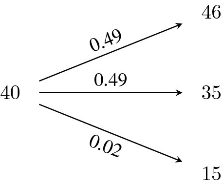
Consider a one-period trinomial tree where a stock evolves as follows:

The one-period risk-free rate is at 4%. You have sold a put option with strike price $37 that expires in one period. You want to manage the risk of your financial position. The payoff of the put option is superimposed to the evolution of the stock price in the tree below.

We do not expect to be able to replicate this put option. However, from our own analyses and experience, we think that the probability of a financial crisis and hence that the stock price crashes to 15$ is only 2%. Therefore, let us ignore this scenario and replicate the put only in the other two normal scenarios, as if it were a binomial model. In other words, let us find the pair solving

We know that the solution to this system is given by

The initial value of this strategy is then given by

By construction, the value of the strategy at time 1 in the normal scenarios is such that

Based upon our judgment, there should be a 98% chance that the portfolio will exactly replicate the payoff of the option at maturity.

But what will happen to this portfolio if a financial crisis occurs? In that case, the time-1 value of the strategy will be equal to

while the put option payoff will be (37 − 15)₊ = 22. In other words, the portfolio will be short by 22 − 5.636363 = 16.36364, with probability 0.02.

The portfolio given by is what we call a sub-replicating portfolio because

in all three scenarios (see also next table).

	Stock	Put	Sub-rep ptf
Value if bull market	46	0	0
Value if bear market	35	2	2
Value if financial crisis	15	22	5.6363
Initial price	40	TBD	0.76923

Consequently, to avoid arbitrage opportunities, this put option must not be sold for a value less than .

 ◼ 

Let us illustrate how to exploit an arbitrage opportunity in this setting.

Example 13.2.4 Exploiting an arbitrage opportunity

In the previous example, we built a sub-replicating portfolio, i.e. a portfolio such that , in all three scenarios. Suppose now that the put option can be bought for only $0.50. Let us explain how to exploit this arbitrage opportunity.

As the option is underpriced, we will buy it and we will short the sub-replicating portfolio. We buy the put option (− 0.50 at inception) and sell the sub-replicating portfolio (+ 0.76923 at inception), for a net initial cash flow of 0.26923. At maturity, if the stock price is either 46 or 35, the net proceeds are zero. However, if the stock market crashes, the strategy yields a profit of 22 − 5.6363 = 16.3637. Therefore, you receive 0.269 at inception, and you will receive a non-negative amount at maturity, thus exploiting this arbitrage opportunity.

 ◼ 

It is also possible to create super-replicating portfolios whose terminal values dominate that of the corresponding option payoff in all scenarios. We illustrate this in the next example.

Example 13.2.5 Super-replication

Your colleague thinks that you should instead replicate the put in the bull market scenario and in the financial crisis scenario only, and therefore ignore the bear market scenario. In other words, she suggests to find the pair solving

We know that the solution to this system of equations is given by

The initial value of this strategy is then given by

By construction, its value at time 1 is such that

But what happens if we set up this portfolio and then the bear market scenario is realized? In that case, the time-1 value of the strategy would be equal to

while the put option payoff would be (37 − 35)₊ = 2. In other words, selling the put and holding this portfolio will generate an extra amount of 7.806454 − 2 = 5.806454, with probability 0.49, and break even the rest of the time.

The portfolio given by is a super-replicating portfolio because

in all three scenarios.

 ◼ 

Let us now illustrate another arbitrage opportunity.

Example 13.2.6 Exploiting an arbitrage opportunity (continued)

In the previous example, we built a super-replicating portfolio, that is a portfolio such that in all three scenarios. Suppose now that the put option can be sold for $4. Explain how to exploit an arbitrage opportunity, if any.

The following table shows the value of the put option and of the super-replicating portfolio in all scenarios.

	Stock	Put	Super-rep ptf
Value if bull market	46	000	0000000
Value if bear market	35	002	7.806454
Value if financial crisis	15	022	0000022
Initial price	40	TBD	3.002484

Selling the put option and buying the super-replicating portfolio will yield an important profit in the bear market scenario. Now if the put option sells for $4 on the market, we can simply sell it and buy the super-replicating portfolio, yielding a profit of nearly $1 at inception (4 − 3.002 = 0.998) and an additional gain when the second scenario realizes. This is an arbitrage opportunity since there is no possibility of loss.

If the put option was sold below $3 (say even $2.99), then the preceding strategy would be a bet that the bear market will occur at maturity. This is no longer an arbitrage opportunity. Therefore, any price below 3.002484 will prevent arbitrage opportunities.

 ◼ 

In the previous examples, there were three pairs of scenarios we could choose from to set up portfolios inspired by our work in the binomial model. There is one such pair we have not looked at. More precisely, what happens if we now decide to ignore the bull market scenario?

We are essentially replicating the scenarios where the put matures in the money. We will be short-selling the stock and investing 35.57692308 at the risk-free rate for a negative initial cost (−4.423076923).³ This is shown in the next table.

This strategy is sub-replicating the payoff of the put option because , in all three scenarios. What this says is that the no-arbitrage price of the put option should be at least −4.423076923, which is not informative since we already found that it should be larger than 0.76923 to avoid arbitrage.

To conclude the above examples, the initial price of the put option should be:

• larger than 0.76923;
• lower than 3.002484;
• larger than −4.4231.

Taking the intersection of the latter three conditions, we find that any price in the interval (0.76923, 3.002484) will not introduce an arbitrage opportunity in this market model.

13.2.3 Super- and sub-replicating strategies

We are now ready to formalize the ideas seen in the previous section. In a one-period trinomial model, we can build three strategies associated to the three pairs of scenarios: (u, m), (u, d) and (m, d). The idea is to ignore one scenario, (temporarily) treat the model as a binomial model and build the corresponding replicating portfolio. These strategies are not replicating strategies for the trinomial model as we are not mimicking the payoffs in all three scenarios.

Out of these three strategies, there always exists at least one super-replicating strategy and at least one sub-replicating strategy. Figure 13.1 illustrates various payoffs that are convex or concave functions of S₁. A line that is located at or above (below) the three points represents a super- (sub-) replicating strategy. The case of call (upper left panel) and put (upper right panel) options is depicted in the upper panels of Figure 13.1. We see that depending on the shape of the payoff function, we might have two sub-replicating strategies and one super-replicating strategies or vice versa.

A super-replicating strategy (or portfolio) for a derivative with payoff V₁ = g(S₁) is a pair such that

in all three scenarios, i.e.

The best super-replicating strategy is the cheapest in the set of all super-replicating strategies. In other words, there might exist many super-replicating strategies for V₁ and the best is simply the one with the lowest cost. We denote the initial value of by .

In the case of call and put options, a quick plot of the payoff function, as in Figure 13.1, suffices to see that there is only one super-replicating portfolio: the one based upon u and d (see the upper panels of Figure 13.1). Therefore, the best super-replicating strategy for a call option is obtained by solving

(13.2.2)

whose unique solution is given by

We can proceed similarly for a put option to find its super-replicating portfolio.

Example 13.2.7

Let us consider again the example where B₁ = 1.1, S₀ = 6 and where the possible values for S₁ are s^u = 7.7, s^m = 5.5 and s^d = 3.3.

In this model, the super-replicating portfolio of a put option with strike K = 6 is given by

And then its initial value is

 ◼ 

A sub-replicating strategy (or portfolio) for a derivative with payoff V₁ = g(S₁) is a pair such that

in all three scenarios, i.e.

The best sub-replicating strategy is the most expensive in the set of all sub-replicating strategies. In other words, there might exist many sub-replicating strategies for V₁ and the best is simply the most expensive. We denote the initial value of by .

Due to the convexity of the payoff of call and put options, there are always two sub-replicating strategies: one based upon scenarios u and m, and another based upon scenarios m and d. However, determining the pair of scenarios yielding the best sub-replicating strategy depends on whether S₀B₁ > s_m or S₀B₁ < s_m. If S₀B₁ < s_m, we should consider m and d.

The methodology is still very similar: select the pair of scenarios u and m, replicate the payoff in those two scenarios and compute the cost of the corresponding sub-replicating portfolio. Then, repeat for the pair of scenarios m and d. This is illustrated in the next example.

Example 13.2.8

Let us consider again Example 13.2.2 where B₁ = 1.1, S₀ = 6 and where the possible values for S₁ are s^u = 7.7, s^m = 5.5 and s^d = 3.3. We know there are two sub-replicating portfolios: one obtained by replicating the payoff with scenarios d and m, and another with scenarios m and u.

The first sub-replicating portfolio is given by

The initial cost of this portfolio is

The second sub-replicating portfolio is given by

with initial cost

As we used suggestive notation, we conclude that the best sub-replicating portfolio is indeed the second one since 0.2272728 > −0.54545.

 ◼ 

What we should remember from this section is that replicating a payoff V₁ in the one-period trinomial tree model almost never leads to a solution (a unique replicating portfolio). Consequently, there is no such thing as a unique price V₀. Most of the time, we will find a range of prices that prevents arbitrage opportunities: any choice of V₀ in the (open) interval will not give rise to an arbitrage opportunity in the trinomial tree. This is also true of incomplete market models in general.

In the rare cases where we can find a unique replicating portfolio, the interval will collapse to a single value

and then we have a unique no-arbitrage price V₀ = Π₀ corresponding to this strategy’s initial value.

Moreover, from a risk management perspective, it is important to understand that the seller of a derivative can no longer be indifferent between:

• buying the equivalent derivative elsewhere on the market (offsetting positions); or
• replicating the liability with basic traded assets.

This is because, in an incomplete market, these two alternatives are not exactly equivalent. Risk management with the second alternative entails some risk.

13.3.1 Maximal and minimal probabilities

Let us recall that in the one-period binomial model of Chapter 9, the price of the replicating portfolio for an arbitrary derivative with payoff V₁ is given by

with

By the no-arbitrage principle, we must have that V₀ = Π₀.

As we saw, it turns out that there exists unique risk-neutral probabilities q and 1 − q, given by

such that

for any derivative with payoff V₁. The risk-neutral probabilities belong to the one-period binomial model, not to a particular derivative.

In the trinomial model, we found that the cost of the best sub-replicating portfolio provides the smallest no-arbitrage price for the corresponding derivative. Even if this portfolio is built to mimick the payoff in only two scenarios, it is still possible to rewrite its cost in terms of a discounted risk-neutral expectation. This will attribute fictitious weights to scenarios u, m and d, similar to what happened in the binomial model. The same can be done for the best super-replicating portfolio.

Let us illustrate the process with call and put options. The cheapest super-replicating portfolio is obtained by considering scenarios u and d, for both options. Hence, we can write

where

Recalling the no-arbitrage condition of (13.1.1), it is clear that . As a consequence, we can also write

where the notation means we are attributing probabilities to scenarios {u, m, d}, respectively.

The best sub-replicating portfolio is obtained by considering scenarios m and d, or scenarios m and u. To illustrate the methodology, suppose that S₀B₁ < s_m, in which case we should consider scenarios m and d. Therefore, we obtain

where

Since we assumed that S₀B₁ < s_m, it is clear that . As a consequence, we can also write

where the notation means we are attributing probabilities to scenarios {u, m, d}, respectively. The methodology is similar when S₀B₁ > s_m, in which case we should consider scenarios m and u.

For convenience, let us define and , as well as and . Then, the range of call option prices such that there are no arbitrage opportunities is given by

while, for the put, it is given by

13.3.2 Fundamental Theorem of Asset Pricing

The approach we just presented can be framed into a more general setting based upon the Fundamental Theorem of Asset Pricing, which is valid for many financial market models such as the binomial model and the trinomial model, as well as the Black-Scholes-Merton model of Chapter 16.

It is beyond the scope of this book to present a formal statement of the FTAP. First, we will present an accessible formulation for binomial and trinomial trees. In Chapter 17, we will present another version for the Black-Scholes-Merton model.

Loosely speaking, the Fundamental Theorem of Asset Pricing states that:

1. a market model is free of arbitrage opportunities if and only if there exists at least one set of risk-neutral probabilities;
2. an arbitrage-free market model is complete if and only if there exists a unique set of risk-neutral probabilities.

In a one-period market model, such as the binomial and trinomial models, we obtain risk-neutral probabilities through the following equation:

(13.3.1)

Equation (13.3.1) is known as the risk-neutral condition.⁴ In other words, risk-neutral probabilities are artificial probabilities such that the risky asset S earns the risk-free rate r on average. Of course, this is not true using real-world probabilities: there is a real rate of return μ for S that is given implicitly by the model parameters. Let us see how the FTAP works in models we already know.

13.3.2.1 One-period binomial model

Let us first illustrate how the FTAP can be applied in the now well-known one-period binomial tree model. First of all, let us assume that the market is free of arbitrage opportunities, i.e. that s^d < S₀B₁ < s_u. In a binomial environment, the risk-neutral condition of equation (13.3.1) is equivalent to

Finding risk-neutral probabilities thus amounts to finding q ∈ (0, 1).

Clearly, we have a unique solution given by

Since there is no arbitrage in this market, we have 0 < q < 1 and also 0 < 1 − q < 1. As expected from the FTAP, under the no-arbitrage assumption, we were able to find a risk-neutral probability. Finally, the risk-neutral probability q is unique and therefore the one-period binomial tree model is a complete market model.

13.3.2.2 One-period trinomial model

In the one-period trinomial model, the risk-neutral condition of equation (13.3.1) is equivalent to

Finding risk-neutral probabilities amounts to finding 0 < q_d, q_m, q_u < 1 such that

(13.3.2)

We have three unknowns, namely q_d, q_m and q_u, but only two conditions, namely the risk-neutral condition of (13.3.1) and the probability condition of (13.3.2). This means there are infinitely many solutions or, said differently, infinitely many different sets of probabilities {q_d, q_m, q_u}.

As expected from the FTAP, since we are assuming the trinomial model is free of arbitrage, we are able to find at least one set of risk-neutral probabilities {q_d, q_m, q_u}.

The converse of the FTAP can be illustrated as follows. Assume there exists a set of risk-neutral probabilities {q_d, q_m, q_u}. This means that 0 < q_u < 1, 0 < q_m < 1 and 0 < q_d = 1 − q_u − q_m < 1, and that

Since {q_d, q_m, q_u} are probabilities, we have that S₀B₁ is a weighted average of the values {s^d, s^m, s^u}, so we have

This is the no-arbitrage condition for the one-period trinomial model.

13.3.3 Finding risk-neutral probabilities

We always assume that the trinomial tree is free of arbitrage, meaning that equation (13.1.1) is verified. Then, the FTAP guarantees the existence of at least one set of risk-neutral probabilities {q_d, q_m, q_u}.

As discussed above, we will find infinitely many risk-neutral triplets {q_u, q_m, q_d} satisfying conditions (13.3.1) and (13.3.2). We have that 0 < q_d, q_m, q_u < 1 are such that

Clearly, we can reduce this to a system of one equation with two unknowns:

or, written differently,

(13.3.3)

In other words, we can parameterize q_u in terms of q_m, or vice versa.⁵ However, we have to make sure that

These last conditions will restrict the range of values for q_u and q_m, i.e. they will not be allowed to vary in the whole interval (0, 1).

The algebra needed to determine all possible risk-neutral triplets {q_u, q_m, q_d} can be tedious but it is elementary, as we will see in the next example.

Example 13.3.1

Let us consider again the example where B₁ = 1.1, S₀ = 6 and where the possible values for S₁ are s^u = 7.7, s^m = 5.5 and s^d = 3.3. As verified earlier, this trinomial model is free of arbitrage, so according to the FTAP, there are risk-neutral probabilities in this model.

The risk-neutral condition in (13.3.1) can be written here as

Collecting the terms for q_u and q_m, we get

If we decide to express q_u in terms of q_m, then we have

and

Our free variable q_m might not be allowed to take any value in (0, 1). We must keep in mind that q_u and q_d, as functions of q_m, must take values in (0, 1):

These two inequalities are equivalent to q_m satisfying both

This means that q_m must be chosen such that

or q_u and q_d might not belong to the interval (0, 1).

In conclusion, we have fully characterized the set of risk-neutral triplets (in terms of q_m). Indeed, for any fixed and arbitrary value of q_m taken in (0, 0.5), the corresponding values for q_u and q_d are given by

For example, if we take q_m = 0.4, then

and we obtain the following risk-neutral triplet .

 ◼ 

13.3.4 Risk-neutral pricing

Now that we know how to obtain risk-neutral probabilities {q_u, q_m, q_d} in a one-period trinomial tree, the next step is to find the interval of no-arbitrages prices as discounted risk-neutral expectations.

Let us denote by a set of risk-neutral probability weights {q_u, q_m, q_d} (meeting the risk-neutral condition). Then, for a random payoff V₁, the discounted risk-neutral expectation

lies within the interval of no-arbitrage prices meaning that

We will not provide a proof of this statement, but the discussion leading to both and should provide the necessary intuition.

This means that for a given risk-neutral probability triplet , the value is a valid no-arbitrage price for the payoff V₁. The notation thus emphasizes that this price depends on the specific choice of risk-neutral triplet .

If the values of q_u and q_d are expressed as functions of q_m, then we will write V₀(q_m) instead of to emphasize that the price is a function of q_m. In other words, we will obtain a parameterized (in terms of q_m) interval of arbitrage-free prices, just as in the super-replication and sub-replication procedure. The next example illustrates the process.

Example 13.3.2

Let us go back to the previous example where B₁ = 1.1, S₀ = 6, s^u = 7.7, s^m = 5.5 and s^d = 3.3. We have fully characterized the set of risk-neutral triplets in terms of q_m: for each 0 < q_m < 0.5, if we set

then the resulting triplet is a set of risk-neutral probabilities.

We would like to find the interval of no-arbitrage prices for a put option with strike price K = 6 and repeat the procedure for a strike price of K = 7.7.

First, if K = 6, then v^u = (6 − s^u)₊ = 0, v^m = (6 − s^m)₊ = 0.5 and v^d = (6 − s^d)₊ = 2.7, and, for a given , we have

As we have chosen to express q_u and q_d as functions of q_m, we further obtain

Clearly, when q_m covers the interval (0, 0.5), the corresponding values of P₀(q_m), which decreases in terms of q_m, will be such that

As we now know, any put option price located within this interval will prevent arbitrage opportunities. We notice that those also correspond to the cost of the best super- and sub-replicating portfolios (see examples 13.2.7 and 13.2.8).

Second, if K = 7.7, then v^u = (7.7 − s^u)₊ = 0, v^m = (7.7 − s^m)₊ = 2.2 and v^d = (7.7 − s^d)₊ = 4.4, and, for a given , we have

In other words, no matter what is the triplet , the interval of no-arbitrage prices for this put collapses to a single value, more precisely P₀ = 1. This should not be a surprise since we were able to exactly replicate this put option.

 ◼ 

Maximal and minimal no-arbitrage prices

It is possible to prove that

where and mean taking the infimum and the supremum over all possible risk-neutral triplets , respectively.

In particular, if q_u and q_d are expressed as functions of q_m, then clearly we have

where means taking the infimum within the possible values for q_m. It is now a minimization problem for a one-variable function. Similarly, we have

13.4.1 Trinomial tree with three basic assets

If we add a third basic asset to the previous trinomial tree model, this asset must be such that:

• it cannot be replicated with the first two basic assets, i.e. it is not a redundant asset;
• it does not introduce any arbitrage opportunities into the market.

From a financial point of view, the first condition amounts to adding a new asset and not just a combination of the previous two basic assets. From a mathematical point of view, we want this asset to help us solve the system of equations associated to the replication problem. Let us illustrate this with an example.

Example 13.4.1 Trinomial model with two stocks

Consider a trinomial market model where two stocks are traded, that of ABC inc. and of XYZ inc., each evolving according to a 3-month trinomial tree. This is illustrated in the trees below.

We should note that the up scenario occurs at the same time for both stocks. We then say the events and are the same. This also holds true for the other two scenarios, meaning that the events and are also the same.

Assume also that the annual interest rate, compounded each 3 months, is at 4%. Thus, we have B₁ = 1.01. We want to find the no-arbitrage price of a 3-month exotic derivative with payoff

In each scenario, the value of this payoff is given by

	V1
u	6.50
m	2.50
d	0

In this modified trinomial model, a trading strategy is a triplet , where (resp. and y) is the number of units of (resp. and B) held in the portfolio from time 0 to time 1. If we want this strategy to replicate the payoff, we must solve:

Subtracting the first two equations and the last two in order to eliminate (1.01)y, we get

Consequently,

Putting these values back into one of the three original equations, we obtain

which yields y = −68.847242. Therefore, the initial value of this replicating portfolio (for this exotic derivative) is given by

By the no-arbitrage principle, this is also the derivative’s initial price.

 ◼ 

In the previous example, we saw a modified version of the trinomial tree model, now with three basic assets, namely B, and . This time, the fact that we were able to replicate the payoff V₁ in a trinomial environment is not coincidental. Since none of the basic assets is redundant, it allowed us to replicate all the risks in the model. Mathematically, this meant solving a system of three equations, associated to the three possible outcomes, with now three unknowns, associated to the three basic assets B, and .

Here is another example where the third asset will be a credit default swap, as seen in Section 4.4 of Chapter 4.

Example 13.4.2 Completing a trinomial market by adding a CDS⁶

Let us have another look at Example 13.0.1. We will introduce a third basic asset, namely a credit default swap (CDS) paying 1$ upon ABC inc.’s default, and 0 otherwise. As we are in a one-period model, assume the CDS requires a single premium at time 0. The following table illustrates the possible realizations of the three basic assets in the three scenarios, along with the payoff of the investment guarantee (IG).

Scenario	Bond B1	Stock S1	CDS CDS1	IG
u	1.04	50	0000	050
m	1.04	30	0000	040
d (default)	1.04	00	1000	040
Initial price	100	40	0.07	TBD

From the table, we have that S₀ = 40 and that CDS₀ = 0.07. Let us see how to use the CDS to manage credit risk and replicate the IG.

Let be the number of shares of the stock, the number of units of CDS and the number of bonds we need to buy to exactly replicate the payoff of the investment guarantee. We need to solve a system of three equations along with three unknowns:

From the first two equations, we directly find and y = 25/1.04 = 24.038461538. This is the same as in example 13.0.1. Now, from the third equation, we find

Therefore, we need to add 15 units of this CDS to the portfolio.

The initial cost of this replicating portfolio (for the IG) is thus

Compared with the strategy deployed in example 13.0.1, for an extra dollar (1.05 to be more precise) the company can completely hedge against credit risk and assure to meet its obligations in all three scenarios.

This is interesting because replicating the first two scenarios might yield a loss of $15 in case of bankruptcy of ABC inc. Therefore, we need to buy the number of CDS required to protect against a possible loss of $15.

 ◼ 

The previous example is pretty realistic in the sense that credit default swaps became commonly traded in the financial markets in the early 2000s. They were one of the many securities that appeared in the markets following the deregulation of financial markets between 1970 and 2000. Securitization is a process commonly used to create tradable securities and it became increasingly important during the same period to help complete the market.

In the insurance business, catastrophe and longevity derivatives, as seen in Chapter 7, can also be viewed as securities helping toward the completion of the insurance market. Natural catastrophe risk and longevity risk were traditionally managed by setting aside an appropriate reserve or with reinsurance. The emergence of these insurance derivatives helped risk managers transfer a significant part of these risks to other investors willing to bear them.