
5
Options
If you hold a long position in a forward contract, you have the obligation to buy the underlying asset at the maturity date, no matter the discrepancy between the delivery price and the price of the asset, if any. In a forward contract, the investor with the short position has the opposite obligation.
In an option contract, the obligation is replaced by the possibility to run away whenever the situation is not profitable. Indeed, if you have the long position in an option to buy, you have the right to buy the underlying asset at the maturity date. Of course, this will be the case only when the delivery price is less than the price of the asset, i.e. only when it is rational to do so. On the other hand, the investor with the short position still has the obligation to sell you this asset. However, this optionality in the option contract comes at a price: a premium must be paid (at inception).
Example 5.0.1 Comparing a forward and an option to buy
Suppose that you can find the following two securities:
- a forward maturing in 3 months and written on a stock with a 3-month forward price of $48;
- an option to buy a stock maturing in 3 months, with a delivery price of $48 and actually trading for $2 (premium).
Let us describe the cash flows in the following two scenarios: in 3 months, the price of the stock will be $45 or it will be $53.
At inception, buying this option requires the payment of a premium of $2 while the forward can be entered at no cost.
In the first scenario, the stock trades for $45. If you have a long position in the forward contract, you are obliged to pay $48 for an asset worth $45, so you lose $3. If you have a long position in this option to buy, you simply use your right not to buy the stock and therefore avoid any cash outflow.
In the second scenario, the stock trades for $53. If you have a long position in the forward contract, you have to pay $48 for an asset worth $53, so you gain $5. If you have a long position in the option, you use your right to buy the stock and also gain $5.
The cash flows are summarized in the next table.
Long forward Option to buy Scenario Stock at maturity CF at inception CF at maturity CF at inception CF at maturity 1 45 0 −3 −2 0 2 53 0 5 −2 5 ◼
Example 5.0.1 contrasts the cash flows of a long forward contract with those of an option to buy.
Options and option-like contracts are very common and can be found outside financial markets. For example, insurance companies sell option-like riders in some of their policies (an important application in life insurance is presented in Chapter 8). You might also have encountered options if you leased a car and have been offered the possibility of buying the car back from the dealer at the end of the contract.
Example 5.0.2 Car lease and buy-back option
You have just signed a contract with a car dealer to lease a brand new vehicle for the next four years (at a given monthly payment). The contract offers the opportunity to buy the car back (from the dealer) at a price of $5,000 once the contract is over. This end-of-lease option is clearly not free: its value is already included in the monthly payments.
At the end of the contract, you analyze the option to buy the car. You go online, look at the ads and feel you could sell the car for $6,000. Therefore, you decide to use the option, i.e. buy the car from the dealer, and then you sell it, for an immediate benefit of $1,000. Suppose instead the market value of the car at the end of the contract is about $4,500. In this case, you will not buy the car from the dealer, as it is an asset worth only $4,500 on the market. In this scenario, you will return the car to the dealer.
◼
The objective of this chapter is to introduce the reader to standard options. The specific objectives are to:
- understand options to buy (call) and options to sell (put) an asset;
- understand the difference between options and forward contracts;
- determine whether an option is used for hedging/risk management or speculating purposes;
- describe various investment strategies using options.
5.1 Framework
After forward contracts, options are the simplest examples of derivatives or contingent claims. A call option (or simply a call) is a financial contract, written on a given asset, that gives its owner the right, but not the obligation, to buy this asset for a given price at a future date (or set of dates). Similarly, a put option (or simply a put) is a financial contract, written on a given asset, that gives its owner the right, but not the obligation, to sell this asset for a given price at a future date (or set of dates). To summarize, a call is an option to buy whereas a put is an option to sell.
The asset on which the option is written is known as the underlying asset and it is specified in the option contract. It could be a security such as a stock or a bond, a commodity, or even a non-financial asset. We say an option is written on an underlying asset because the option gets its value from that asset.
The price at which the underlying asset can be bought or sold upon exercise is also specified in the contract. It is called the strike price, the exercise price or even the delivery price (as in forward contracts). This is similar to the delivery price in forward/futures contracts but with options, delivery might not take place. Buying or selling the underlying asset is known as exercising the option.
Finally, the duration, or life, of the option is also specified in the option contract. The date when the contract is initiated, i.e. the issuance date, is known as inception whereas the last day when the option can be exercised is called maturity, the maturity date or expiry date.
As discussed in Chapters 2 and 3, we will use the words owner and buyer (of the option) interchangeably to represent the investor with the long position in the option (long option holder), and the words writer and seller (of the option) for the investor with the short position (short option holder). One has to be careful with the terminology: it is possible to buy options to sell (put options) and sell options to buy (call options).
As seen above, not being required to exercise an option has value because the owner can avoid losing money at maturity. Therefore a premium must be paid at inception, or a price must be paid at later times, to acquire an options contract. Options commonly traded on financial markets require an up-front premium but many options-like riders found in insurance policies are paid during the life of the contract.
Therefore, options generate cash flows at two specific moments:
- At inception, the option buyer pays a premium to the option seller.
- At maturity, if the option is exercised, the asset and an amount of cash will be exchanged by the two parties involved. The net value is known as the option payoff.
The profit (or loss when negative) from buying or selling an option is the amount received, net of the amount paid. For example, when buying an option, the profit is calculated as the payoff net of the premium and when selling an option, the profit is the premium that we receive net of the payoff that we owe. Note that we do not take into account the time value of money; for most options, maturities are relatively short.
An option contract also requires to specify when, during the life of the option, exercise may happen. There are three categories:
- when an option can be exercised only at maturity, the option is said to be European;
- when an option can be exercised at any date between inception and maturity, the option is said to be American;
- when an option can be exercised on given dates between inception and maturity, the option is said to be Bermudan.
For example, an American put option gives its holder the right to sell the underlying asset for the strike price anytime before maturity.
Options’ names
One may also wonder why some options’ names are linked to a continent, country or city. Modern financial history generally dates back to the early 1970s with the creation of options markets in the U.S. However, option-like contracts were created long before the 20th century.
Typical option-like contracts traded in Europe in the 17th century could be exercised at maturity only whereas American option-like contracts traded in the U.S. in the late 18th century could be exercised anytime before maturity []. The names European and American options were popularized by the economist Paul Samuelson.
The name Bermudan option was coined because Bermuda is geographically located between Europe and the U.S. but closer to the U.S. (a Bermudan option is indeed closer to an American option than to a European option). There is also the Asian option, which is a type of exotic option whose payoff is determined by the average price (see Chapter 7). The name comes from the traders who were in Tokyo in the late 1980s when they developed the methodology to price such options.
The relationship between the asset price and the strike price determines the option’s current intrinsic value and its moneyness. The intrinsic value of an option is the amount that would be received today if the option were exercised, regardless of whether such an exercise is allowed. The moneyness of an option is given by the relative positions of the underlying asset’s price and the strike price. More precisely, an option is said to be:
- in the money if the intrinsic value is positive;
- out of the money if the intrinsic value is negative;
- at the money if the intrinsic value is zero.
Therefore, when an option is exercised at maturity, the intrinsic value and the payoff are equivalent.
In what follows, we will analyze standard call and put options only, also known as vanilla options. Unless stated otherwise, we will consider only European calls and puts whereas American options will be investigated in Chapter 6.
5.2 Basic options
As before, one should think of time 0 as today, while any other time t, for t > 0, is set in the future. The evolution of the price of a given asset (stock, index, commodity, etc.) will be represented by S = {St, t ≥ 0}, where St stands for its (future) time-t price. In particular, S0 is today’s spot price, the price at which the asset is currently traded.
We will use the following notation for the main features of an option written on S:
- K is the strike price;
- T is the maturity date.
In other words, this option is struck at K and matures at time T.
The underlying asset price at the option’s expiry is given by ST. As of today, this value is unknown, because it is set in the future. Therefore, ST is a random variable, and so is St, for any other t > 0.
5.2.1 Call options
A call option gives the right to buy the underlying asset S for a price of K at time T. At maturity, there are two possibilities:
- If ST is less than K, then the option is out of the money. Buying the asset for K is not reasonable and the option is left unexercised.
- If ST is greater than K, then the option is in the money. Buying the asset for K is rational and the option is exercised.
Figure 5.1 illustrates the cash flows between the buyer and the seller of the call option. If ST > K, then the option’s buyer pays K to the option’s seller in exchange for an asset worth ST. Overall, the buyer’s wealth has increased by an amount of ST − K.

Figure 5.1 Exchanges between the buyer and the seller of a call option at maturity for a physical settlement
When the asset is delivered to the call option buyer, we say the call is physically settled (physical settlement). Instead of delivering the asset, the call option seller could simply pay the cash equivalent of ST − K upon exercise. This is known as cash settlement. Cash settlement is illustrated in Figure 5.2.

Figure 5.2 Exchanges between the buyer and the seller of a call option at maturity for a cash settlement
For a liquid asset, physical and cash settlements are equivalent. Indeed, upon delivery of the asset, the call option owner could immediately sell the asset in the market and receive ST in cash. Recall that we assume all assets are liquid.
Regardless of the type of settlement, the payoff of a long call option is given mathematically by
Here, we used the following mathematical function: (x)+ = max (x, 0). In other words, for any given real number x, this function returns x if it is a positive number, otherwise it returns 0.
Recall that entering the long position in a call requires the payment of an up-front premium C0 > 0. The following table summarizes the cash flows occurring at time 0 (inception) and at time T (maturity) for a long call option.
| Time/Scenario | ST < K | ST > K |
| time 0 (inception) | − C0 | − C0 |
| time T (maturity) | 0 | ST − K |
We observe that no matter the scenario, the option buyer has to pay the premium, while the (random) payoff of the option depends on the terminal value ST of the underlying asset. The upper-left plot of Figure 5.3 also shows the payoff and profit diagrams for a long call option.

Figure 5.3 Payoff (continuous line) and profit (dashed line) of long/short call and put options
A long call option with strike price K has all the upside benefits of a long forward contract with delivery price K without the downside risk. However, an up-front premium needs to be paid by the long call option holder.
Example 5.2.1 Long call option
A 6-month European call option on a stock has just been issued. The call has a strike price of $55 and currently trades at $2.50. Let us describe the cash flows of a long position in this option for the following two scenarios: if the stock trades at $60 or if it trades at $50, 6 months from now.
At inception, the long call option holder needs to pay the premium of $2.50.
At maturity, if the stock price is at $60, then the option will provide the possibility to buy the stock at $55 rather than at $60. This payoff is equal to $5 and the corresponding profit is equal to $2.50.
At maturity, if the stock price is at $50, the option will not be exercised. The payoff is thus equal to $0 and the corresponding profit in this case is a loss of $2.50.
The cash flows are summarized in the table.
Time/Scenario ST = 50 ST = 60 At inception − 2.50 − 2.50 At maturity 0 60 − 55 = 5 ◼
We now take the point of view of the option writer, i.e. the investor with the short position in the call option. For this investor, all cash flows are reversed, as shown in the following table.
| Time/Scenario | ST < K | ST > K |
| time 0 (inception) | + C0 | + C0 |
| time T (maturity) | 0 | − (ST − K) |
Indeed, the option seller always receives a premium at inception but if the call option is exercised by the buyer, then the writer needs to deliver a unit of the asset and will receive K in exchange. The interactions between the option buyer and seller are summarized in Figures 5.1 and 5.2. Moreover, the lower left plot of Figure 5.3 shows the payoff and profit diagrams for a short call option.
Mathematically, the payoff of a short call option can be written as
Example 5.2.2 Short call option
Using the values and scenarios provided in example 5.2.1, let us describe the cash flows of a call option writer.
At inception, the option seller receives a premium of $2.50.
If the stock price goes down to $50, then the option buyer will not exercise the option. In this scenario, the payoff will be $0 and the profit for the option seller will be $2.50.
If the stock price goes up to $60, then the option buyer will exercise the option. This means the option seller will have to deliver a share of stock worth $60 in exchange for $55. In this scenario, the payoff will be −$5 and the corresponding loss will be $2.50.
The cash flows are summarized in the table.
Time/Scenario ST = 50 ST = 60 At inception + 2.50 + 2.50 At maturity 0 − (60 − 55) = −5 ◼
5.2.2 Put options
A put option gives the right to sell the underlying asset S for a price of K at time T. At maturity, there are two possibilities:
- If ST is less than K, then the option is in the money. Selling the asset for K is rational and the option is exercised.
- If ST is greater than K, then the option is out of the money. Selling the asset for K is not reasonable and the option is left unexercised.
Figures 5.4 and 5.5 illustrate the cash flows between the buyer and the seller of the put option. If ST < K, then the option’s buyer receives K from the option’s seller in exchange for an asset worth ST. Overall, the buyer’s wealth has increased by an amount of K − ST.

Figure 5.4 Exchanges between the buyer and the seller of a put option at maturity for a physical settlement

Figure 5.5 Exchanges between the buyer and the seller of a put option at maturity for a cash settlement
Mathematically, the payoff of a long put option is given by
Here are the cash flows of a put option buyer:
| Time/Scenario | ST < K | ST > K |
| time 0 (inception) | − P0 | − P0 |
| time T (maturity) | K − ST | 0 |
Also, the upper-right plot in Figure 5.3 shows the payoff and profit diagrams for a long put option.
A long put option with strike price K has all the benefits (if the underlying asset price goes down) of a short forward contract with delivery price K without the disadvantages (if the underlying asset price goes up). However, an up-front premium needs to be paid by the long put option holder.
Example 5.2.3 Long put option
A 4-month European put option on a stock has just been issued. The put has a strike price of $60 and currently trades at $3. Let us describe the cash flows of a long position in this option for the following two scenarios: if the stock trades at $55 or if it trades at $65, 4 months from now.
At inception, the long put option holder needs to pay the premium of $3.
At maturity, if the stock price is at $65, then the option will provide the possibility to sell the stock at $60 rather than at $65. The option will not be exercised, so the payoff is equal to $0 and the corresponding loss is equal to $3.
At maturity, if the stock price is at $55, then the investor with the long position is allowed to sell for $60 a stock worth $55. The payoff is $5 and the profit is then $2.
The cash flows are summarized in the next table.
Time/Scenario ST = 55 ST = 65 At inception −3 −3 At maturity 60 − 55 = 5 0 ◼
Taking the point of view of the put option seller, then again all cash flows are reversed as shown in the following table.
| Time/Scenario | ST < K | ST > K |
| time 0 (inception) | + P0 | + P0 |
| time T (maturity) | − (K − ST) | 0 |
Based upon Figure 5.4, we see that the investor with the long position in the put option will deliver/sell a share of the underlying asset for K (to the investor with the short position in the put option) only if K > ST. Therefore, the investor with the short position in the put option will effectively be buying a unit of the asset for K. This is done in exchange for an up-front premium that the seller has received at inception. The bottom-right plot of Figure 5.3 shows the payoff and profit diagrams for a short put option.
Mathematically, the payoff of a short put option can be written as
Example 5.2.4 Short put option
Using the values and scenarios provided in example 5.2.1, let us describe the cash flows of a put option writer.
At inception, the investor issuing the put option receives a premium of $3.
At maturity, if the stock price ends up at $65, then the put option would provide its buyer with the possibility to sell the stock for $60 (rather than $65). Of course, she will abandon this possibility. The payoff from the seller’s perspective is zero and the profit in this scenario would be $3, i.e. the value of the initial premium.
At maturity, if the stock price ends up at $55, then the option buyer will exercise its right of selling a share of stock for $60 (rather than $55). Therefore, the put option buyer delivers one share of stock to the option seller in exchange for $60. The payoff is −5 and the loss is $2.
The cash flows are summarized in the next table.
Time/Scenario ST = 55 ST = 65 At inception + 3 + 3 At maturity − (60 − 55) = −5 0 ◼
5.3 Main uses of options
In Chapter 2, we mentioned the two main uses of derivatives – including of course options – which are hedging/risk management and speculation. The main difference between the two is in how the profits from the option are used: to offset a potential loss (hedging) or to magnify a potential gain (speculation).
5.3.1 Hedging and risk management
Options can be used for hedging, i.e. to attenuate risks as part of a risk management strategy. Insurance companies and pension plan sponsors have assets and liabilities that are exposed to variations in stock prices, interest rates, exchange rates, etc. They can use options to help mitigate those risks. As mentioned already in Chapter 2, when insurance companies use derivatives (including options), they mostly use them for hedging purposes.
Example 5.3.1 Protective put
Suppose the assets of a pension plan will decrease (resp. increase) significantly if the price of a stock goes down (resp. up). This is similar to being long that stock. As the investment actuary of that pension plan, you are interested in keeping the upside potential of your investment but you are seeking protection against the downside risk.
A long put option can play this role. In exchange for an up-front premium P0, the put option gains whenever the stock price goes down whereas the payoff is zero otherwise. The next table shows how we can hedge a long stock position by simultaneously being long a put option.
Security/Scenario ST ≤ K ST > K Long stock ST ST Long put K − ST 0 Total K ST We see from this table that buying a put option essentially limits the losses due to a drop in the stock price. It sets a lower limit on the portfolio value and this is why it is also known as a floor. The put option acts as an insurance on the long stock position and an up-front premium is required for this insurance. This strategy is also known as a protective put.
◼
Example 5.3.2 Call option for hedging purposes
Suppose now that an investor is exposed to variations in the stock price such that she loses if the price goes up. This can be the case whenever an investor has shorted a stock she needs to buy back later. Indeed, she benefits whenever the stock price goes down but she is severely hit if the stock price goes up. Obviously, this investor would want to continue to profit from stock price decreases but limit losses if the stock price goes up. A long call option can play this role. In exchange for an up-front premium of C0, the call option profits whenever the stock price goes up whereas the payoff is zero otherwise. The next table shows how we can hedge a short stock position with a long call option.
Security/Scenario ST ≤ K ST > K Short stock − ST − ST Long call 0 ST − K Total − ST − K It is important to insist that, at inception, the investor will receive S0 − C0 > 0, which is the result of the short sale net of the cost of the call option. At maturity, the cash outflow is either ST or K, whichever is the smallest. Note that in the scenario where ST > K, the final payoff is − K which in this case is greater than − ST.
The short stock position is costly if the stock price increases so the call option caps at K the price at which the stock will have to be bought back. The call option acts as an insurance on the short stock position by limiting losses and this is why it is called a cap. Therefore, an up-front premium is required for this insurance.
◼
Covered and naked options
For an option writer, a covered option is simply a short option combined with an offsetting position in the underlying asset, as opposed to a naked option which is just the short option.
We know that a call option writer should be prepared to deliver a share of stock if the option is exercised at maturity. Therefore, a naked call is simply a short call whereas a covered call is a strategy combining a short call and a long stock. In this case, if exercise occurs at maturity, the call option writer can deliver the share of stock he already owns. The payoff of a covered call is summarized in the following table.
| Security/Scenario | ST ≤ K | ST > K |
| Long stock | ST | ST |
| Short call | 0 | − (ST − K) |
| Total | ST | K |
Similarly, a put option writer should be prepared to buy a share of stock if the option is exercised. Therefore, a naked put is simply a short put option whereas a covered put is a strategy combining a short put and a short stock. In this case, if exercise occurs at maturity, the put option writer will cover its short position in the stock. The payoff of this strategy is summarized in the following table.
| Security/Scenario | ST ≤ K | ST > K |
| Short stock | − ST | − ST |
| Short put | − (K − ST) | 0 |
| Total | − K | − ST |
Although the final payoffs are negative, the investor receives a substantial income of S0 + P0 at inception.
5.3.2 Speculation
To speculate means taking investment positions to profit from anticipated asset price movements. It can also be interpreted as a bet because even though we believe the stock price will go up or down, it might not happen.1 Therefore, an investor can use calls (resp. puts) to speculate that the stock price will go up (resp. down) in the future.
Example 5.3.3 Call option for speculation purposes
Suppose you have $1000 to invest. A share of a stock trades at $100 and a 3-month at-the-money call trades at $5. Assume for simplicity that the stock price can only increase and end up at $125 or decrease and end up at $75 in 3 months.
You have analyzed the risk-return profile of this stock and truly believe its price will increase to $125. You want to compare two investment opportunities:
- $1000 worth of stocks;
- $1000 worth of call options on that stock.
Buying 10 shares of stock costs $1000. If your prediction is realized, then it will yield a profit of $250 in 3 months ($25 per share). On the other hand, $1000 also buys 200 call options. For this other financial position, if your prediction is realized, then the payoff would be $25 per option and the profit would be of $20 per option or $4000 in total. The profit of this second investment opportunity is much larger than the first one, if your prediction is realized.
Call options provide what is known as leverage because you would need to buy 20 shares of stock to have the same gain as a single call option. It is important to note that if your prediction is not realized and the stock price goes down to $75, the loss incurred by buying the stocks is limited to $250, but with 200 call options, you would lose your entire investment, i.e. $1000.
◼
Example 5.3.4 Put option for speculation purposes
Whenever an investor believes the stock price of a company will go down, she can speculate by:
- shorting the stock; or
- buying a put option.
Suppose the current stock price is $50 and it can only increase to $60 or decrease to $40 6 months from now.
Let us begin by looking at what happens if we short the stock. We receive $50 by selling the stock today, knowing we will have to buy it back in 6 months. If the stock price were to decrease to $40, we would make a profit of $10 but, if the stock price were instead to increase to $60, we would suffer a loss of $10.
Suppose there is an at-the-money put option available (i.e. with a strike price of $50) for a premium of $4. We buy one unit of this option. If the stock price decreases to $40, we will exercise the option, i.e. sell at $50 and immediately buy one stock at $40, for a payoff of $10. The profit is $6 and we will have a return on investment of 150%. But if the stock price goes up, the option will be left unexercised and we will lose the entire investment of $4, for a return of −100%.
◼
In conclusion, buying call and put options instead of buying or short-selling the underlying asset amplifies the exposure to changes in the asset price, which is known as the leverage effect. We need to remember that it exaggerates both gains and losses.
5.4 Investment strategies with basic options
The previous section showed that a put (or a call) option can be used to profit from a price drop (increase) in the underlying asset. We now look at how to use combinations of options to benefit from, or protect our position against, different types of movements of the underlying asset price. In what follows, unless stated otherwise, all options are written on the same underlying asset S and have the same maturity date T.
Bull spreads
A bull spread is a strategy that benefits when the price of the underlying asset goes up. Instead of buying a single call option, the idea of a bull spread is to reduce the overall cost by reducing the upside potential. Therefore, a bull spread consists in buying a call with strike price K1 and selling an out-of-the-money call with strike price K2, where K1 < K2. The payoff of the bull spread is given by
and is illustrated in Figure 5.6.

Figure 5.6 Payoff (continuous line) and profit (dashed line) of various strategies involving options
Compared with buying only a call option with strike price K1, selling the call option with strike price K2 reduces the upside benefit but also reduces the initial cost. Indeed, the lower the strike price, the higher the value of the call. The cash flows at maturity are summarized in the following table.
| Security/Scenario | ST ≤ K1 | K1 < ST < K2 | ST ≥ K2 |
| Long call with K1 | 0 | ST − K1 | ST − K1 |
| Short call with K2 | 0 | 0 | − (ST − K2) |
| Total | 0 | ST − K1 | K2 − K1 |
Note that it is also possible to obtain a similar payoff by combining put options. When the bull spread is constructed with call (resp. put) options, it is referred to as a bull call (resp. bull put) spread.
Bear spreads
A bear spread is a strategy that benefits when the price of the underlying asset goes down. Instead of buying a single put option, the idea of the bear spread is to reduce the overall cost by reducing the upside potential. Therefore, a bear spread consists in buying a put with strike price K2 and selling an out-of-the-money put with strike price K1, where K1 < K2. Its payoff is given by
and is illustrated in Figure 5.6.
Compared with buying only a put option with strike price K2, selling the put option with strike price K1 reduces the upside benefit but it reduces also the initial cost. The cash flows at maturity are summarized in the following table.
| Security/Scenario | ST ≤ K1 | K1 < ST < K2 | ST ≥ K2 |
| Short put with K1 | − (K1 − ST) | 0 | 0 |
| Long put with K2 | K2 − ST | K2 − ST | 0 |
| Total | K2 − K1 | K2 − ST | 0 |
A similar payoff can be obtained by combining call options. When a bear spread is built with puts (resp. calls) it is sometimes referred to as a bear put (resp. bear call) spread.
Note that the words bull and bear refer to a common terminology used by investors to designate a market that is expected to go up (bull market) or down (bear market).
Ratio spreads
We can generalize bull and bear spreads by buying n options with strike price K1 and selling m options with strike price K2. This strategy is known as a ratio spread and can be built with m + n calls or m + n puts.
Ratio spreads are usually quoted using the notation n: m designating the ratio of the number of options bought and sold. Since m and n are flexible, it is possible to build a zero-cost ratio spread.
Variations on the ratio spread
There are other spread strategies that are similar in spirit to a ratio spread:
- A vertical spread is a ratio spread with m = n.
- A box spread can be obtained by combining a bull spread and a bear spread. It results in a risk-free position of K2 − K1.
- A butterfly spread is a strategy that involves buying two calls, one with strike K1 and another with strike K2, in addition to selling two calls with strike K, where K1 < K < K2.
Straddle
A straddle is a strategy used when (large) movements, upward or downward, in the price of the underlying asset are expected. It consists in buying a call and a put with the same strike price. The payoff of the strategy is then given by
as illustrated in Figure 5.7.

Figure 5.7 Payoff (continuous line) and profit (dashed line) of a straddle
With such a strategy, we benefit when ST is far from K, but we have to pay C0 + P0. The cash flows at maturity are summarized in the following table.
| Security/Scenario | ST ≤ K | ST > K |
| Long call | 0 | ST − K |
| Long put | K − ST | 0 |
| Total | K − ST | ST − K |
Strangle
We can generalize a straddle: it is called a strangle. This strategy can be used when (large) movements, upward or downward, in the price of the underlying asset are expected, but with a reduced cost.
A strangle consists in buying a call and a put option with different strike prices. More precisely, the strangle involves buying a call with a strike price K2 > K and a put with strike price K1 < K. Both options are cheaper than their equivalent with a strike of K.
The payoff of the strategy is then given by
and is illustrated in Figure 5.6.
With such a strategy, we benefit when ST is outside the interval (K1, K2). Again, we have to buy two options, but it is cheaper than a straddle with strike price K. The cash flows at maturity are summarized in the following table.
| Security/Scenario | ST ≤ K1 | K1 < ST < K2 | ST > K2 |
| Long put with K1 | K1 − ST | 0 | 0 |
| Long call with K2 | 0 | 0 | ST − K2 |
| Total | K1 − ST | 0 | ST − K2 |
Clearly, if K1 = K2, then we recover a straddle.
Collar
A collar consists in buying a put with strike price K1 and selling a call with strike price K2, where K1 < K2. The difference K2 − K1 is known as the collar width. Its payoff is given by
Note that the payoff at maturity can take negative values. The payoff and profit of a collar are shown in Figure 5.6. The cash flows at maturity are summarized in the following table.
| Security/Scenario | ST ≤ K1 | K1 < ST < K2 | ST > K2 |
| Long put with K1 | K1 − ST | 0 | 0 |
| Short call with K2 | 0 | 0 | − (ST − K2) |
| Total | K1 − ST | 0 | − (ST − K2) |
A zero-cost collar is a collar such that strike prices are adjusted to have a zero initial cost. One possible case is when both K1 and K2 are equal to the forward price of the underlying asset. More details are given in the next chapter.
5.5 Summary
Options
- Underlying asset: S.
- Strike/exercise price: K.
- Maturity/expiry date: T.
- Provide the right, rather than the obligation, to buy/sell the asset S, for the strike price K, at maturity T.
- Difference from forwards/futures:
- – right to buy/sell the asset, not an obligation.
- – a premium must be paid.
Types of exercises
- European option: exercise is allowed only at maturity.
- American option: exercise is allowed anytime before or at maturity.
- Bermudan option: exercise is allowed only on pre-specified dates before or at maturity.
Payoff and profit
- Payoff: net value at maturity.
- Profit: payoff minus the premium.
Intrinsic value and moneyness
- Intrinsic value: amount that would be received today if the option were exercised, regardless of whether such an exercise is allowed.
- Moneyness: at any given time, an option is
- – in the money: if the intrinsic value is positive;
- – out of the money: if the intrinsic value is negative;
- – at the money: if the intrinsic value is zero.
Settlement
- Physical settlement: asset and strike price are physically exchanged between the option buyer and the option seller.
- Cash settlement: payoff is paid in cash.
Call options
- Provide the right to buy the underlying asset S for the strike price of K at maturity time T.
- Premium: C0.
- Payoff: (ST − K)+ = max (ST − K, 0).
- Intrinsic value at time t: (St − K)+ = max (St − K, 0).
Put options
- Provide the right to sell the underlying asset S for the strike price of K at maturity time T.
- Premium: P0.
- Payoff: (K − ST)+ = max (K − ST, 0).
- Intrinsic value at time t: (K − St)+ = max (K − St, 0).
Calls, puts and forward contracts
| Position/Scenario | ST < K | ST > K |
| Long call | 0 | ST − K > 0 |
| Short call | 0 | − (ST − K) < 0 |
| Long put | K − ST > 0 | 0 |
| Short put | − (K − ST) < 0 | 0 |
| Long forward | ST − K < 0 | ST − K > 0 |
| Short forward | K − ST > 0 | K − ST < 0 |
Main uses
- Hedging: attenuate risks as part of a risk management strategy; the gain is used to offset a potential loss.
- – Protective put, i.e. long stock + long put option: puts a lower limit on the portfolio value (floor).
- – Short stock + long call: puts an upper limit on the amount required to cover the short stock position (cap).
- Speculation: taking investment positions to profit from anticipated asset price movements.
Investment strategies with basic options
- Assumption: K1 < K < K2.
- Bull spread, i.e. long call K1 + short call K2:

- Bear spread, i.e. long put K2 + short put K1:

- Ratio spread, i.e. long n options K1 + short m options K2 (options should be of the same type):
or


- Straddle, i.e. long call K + long put K:

- Strangle, i.e. long call K2 + long put K1:

- Collar, i.e. long put K1 + short call K2:

5.6 Exercises
-
Butterfly spread
A butterfly spread is a strategy that involves buying one call each with strikes K1 and K2 and selling two calls with strike K, where K1 < K < K2. Note also that we should have K2 − K = K − K1.
- Detail in a table the payoff of each call option and the total payoff of the strategy.
- Plot the payoff diagram for this strategy.
- Describe the scenarios where the butterfly spread would be valuable.
-
Strips and straps
A strip combines one call option with two put options, whereas a strap combines two call options with one put. In all cases, the strike price is K. For the strip and the strap:
- Detail in a table the payoff of each option and the total payoff of the strategy.
- Plot the payoff diagram for this strategy.
- Describe the scenarios where strips and straps would be valuable.
-
Covered and naked options
- A stock currently trades for $50 whereas a 1-month at-the-money call option on that stock trades for $2. Assume that over the next month the stock price can only increase to $55 or decrease to $45. Describe the payoff and profit at maturity for a naked call and a covered call.
- Suppose a 1-month at-the-money put option trades at $2 as well (for simplicity). Describe the payoff and profit at maturity for a naked put and a covered put option.
-
Options and forwards
- Suppose that in the context of example 5.2.1, a forward contract is also available for a delivery price of $55. Compare the cash flows from a short forward and a short call option position.
- In the context of example 5.2.3, compare the profits from a long forward contract or a short put option.
-
Comparing a long call option and a long forward contract
Suppose that in the context of example 5.2.1, a forward contract is also available for a delivery/forward price of $55 with delivery in 6 months. Compare the cash flows of a long forward and a long call along with the payoff and profit from these positions.
-
Comparing a long put option and a short forward contract
In the context of example 5.2.3, suppose a forward contract is also available such that the 4-month forward price is $60. Compare the cash flows of a short forward contract with those of a long put option along with the payoff and profit from these positions.
-
Investment strategies
What securities, or combinations thereof, would you use to gain from each of the following situations?
- ABC inc. is being sued for patent infringement on an important product it sells. The court will make its decision public within 3 months. Its decision, positive or negative, is likely to affect future profitability of the company.
- Rumors are persistent on the bankruptcy of ABC inc.
- The government intends to tax sugar. Suppose ABC inc. refines sugar.
-
A box spread combines bull and bear spreads.
- Show that a box spread results in a risk-free position of K2 − K1.
- What should be the no-arbitrage price of this box spread?
- When is the box spread costless at inception?
-
Collars
- What is the no-arbitrage price of a collar such that K = K2 = K1?
- Show that when K corresponds to the T-forward price of the underlying asset, then the collar has zero cost.
-
Comparing options with different strike prices
Suppose we analyze two call options with strike prices K1 < K2. Let C10 and C20 be the up-front premiums for these two call options.
- Explain intuitively why C10 should be higher than C20.
- Using no-arbitrage arguments, show that C10 > C20.
-
Heartbeat option
A heartbeat option is a totally fake option whose payoff diagram is given in Figure 5.8. Reverse engineer this option to find a strategy that exactly replicates the latter payoff diagram. Hint: butterfly.
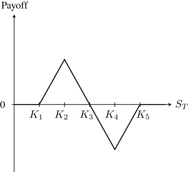
Figure 5.8 Payoff of a heartbeat option
-
Zero-cost ratio spread
A 40-strike call option currently sells for $4.25 whereas a 42-strike call options trades for $3.75. A ratio spread can be built by buying n 40-strike call options and selling m 42-strike call options. Find the range of values of m and n such that the ratio spread is costless at inception.