
3
Forwards and futures
In many situations, it is good risk management to fix today the price at which an asset will be purchased in the future. Here are two examples:
- Consider a company regularly buying gold as an input for its business, e.g. that company could transform gold to make jewelry. This company is clearly exposed to the (random) fluctuations of the gold price. More specifically, it would suffer from an increase in the price. In this case, it may be a good idea to enter into a financial agreement that fixes the price of gold today for delivery in the future. Therefore, the cost of jewelry made over the next few weeks/months can be known in advance.
- An insurance company based in the U.S. but also doing business in Canada is exposed to changes in the currency rate between the U.S. dollar (USD) and the Canadian dollar (CAD). It could enter into a financial agreement to fix today the exchange rate between these currencies that will apply in the future.
Forward contracts and futures contracts can be used specifically for this purpose: fix today the price of a good to be bought in the future. They are also commonly known as forwards and futures, without the word contract or agreement attached to them.
The role of this chapter is to provide an introduction to forwards and futures. The specific objectives are to:
- recognize situations where forward contracts and futures contracts can be used to manage risks;
- understand the difference between a forward contract and a futures contract;
- replicate the cash flows of forward contracts written on stocks or on foreign currencies;
- calculate the forward price of stocks and of foreign currencies;
- calculate the margin balance on long and short positions of futures contracts.
3.1 Framework
This section lays the foundations of forwards and futures for the rest of the chapter. The content applies regardless of the underlying asset.
3.1.1 Terminology
A forward contract or a futures contract is a contract that engages one party to buy (and the other to sell) an asset some time in the future for a price determined today at inception of the contract. That time in the future is known as the expiration, maturity or delivery date whereas the said price is known as the delivery price.
The most important difference between forwards and futures is that futures are standardized and exchange-traded. Exchanges require investors to hold money aside to protect both sides of the transaction from default risk. This is usually known as the process of marking-to-market. This difference aside, forwards and futures serve the same purpose: fixing today the price at which an asset will be bought in the future.
Forward contracts and futures contracts also differ from spot contracts:
- A spot contract is agreed upon today between a buyer and a seller, the asset is paid for and delivered (almost) immediately.
- A forward (futures) contract is also agreed upon today but the asset will be paid for and delivered at maturity of the forward (futures) contract.
Therefore, if you need to acquire the asset, say in 3 months, then instead of waiting 3 months and buying the asset on the spot market and paying a price viewed as random today, the forward contract fixes that price today.
To simplify the presentation of this chapter, we will start by looking at forward contracts and we will come back to futures contracts in Section 3.5.
3.1.2 Notation
Let us begin with the following standard notation:
- K is the delivery price;
- T is the maturity date.
We say that delivery of the underlying asset will occur at time T or that the forward contract will mature at time T.
Entering the long position of a forward contract, or said differently buying a forward contract, does not usually require an initial payment/premium. However, to avoid arbitrage opportunities, this restriction will have an impact on the right value of K. For now, we will consider that K can take any value and that entering a forward contract might require, or not, an upfront payment. We will come back to this issue later when we discuss the forward price.
The cash flows of a forward contract are:
- At inception (at time 0), both parties agree on K (and on T) and an up-front premium might be required (paid by the forward buyer (long position) to the forward seller (short position)), or vice versa.
- At maturity (at time T), the investor with the long position pays K and receives the underlying asset worth ST from the investor with the short position, no matter what the realization of the random variable ST is. This is illustrated in Figure 3.1.
Figure 3.1 Cash flows of a forward contract at maturity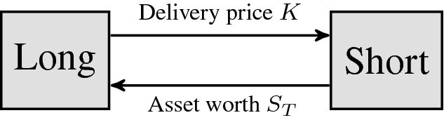
3.1.3 Payoff
In general, the payoff of a derivative corresponds to its value at maturity. Usually, it is the net amount received by the investor with the long position. For a forward contract, the payoff can be positive (gain), negative (loss) or zero. Mathematically, the payoff of a long forward is given by
which is positive if ST > K, but is negative otherwise. Therefore, the payoff of a short forward is given by
The payoff of a long or a short position in a forward contract is illustrated in Figure 3.2 as a function of the terminal value of the underlying asset, i.e. as a function of ST.
No matter the perspective (either long or short position), the payoff of a forward contract is random. Indeed, as of today, it is impossible to determine whether it is beneficial for either party to fix today the buying or selling price of the asset.
Example 3.1.1 Payoff of a forward on a stock
A stock currently trades at $65. You intend to buy this stock 3 months from now and you would like to fix the buying price today. Therefore, you choose to enter the long position in a forward contract with a delivery price of $67 and a maturity date in 3 months. Assume it costs nothing at inception to enter this forward contract.
Let us determine the gain/loss of the long forward if the stock price reaches $70 or if it remains at $65 in 3 months.
At time 0, there are no cash flows. At maturity, in the first scenario, you have to buy an asset worth $70 for only $67. Therefore, the gain is 70 − 67 = 3. In the second scenario, you have to buy an asset worth $65 for $67, which is a gain of 65 − 67 = −2. In other words, in this second scenario, it is a loss of $2. ◼

Figure 3.2 Payoff of a long forward (continuous line) and a short forward (dotted line)
Just like a long (resp. short) position in an asset, the value of a long (resp. short) position in a forward contract written on this same asset increases (resp. decreases) whenever the price of the underlying asset increases (resp. decreases).
3.2 Equity forwards
In this section, we will analyze equity forwards, also known as forwards on stocks. We will consider stocks:
- not paying dividends;
- paying discrete and fixed dividends;
- paying continuous and proportional dividends.
3.2.1 Pricing
Our first objective is to find the no-arbitrage value of a long forward contract with delivery date T and delivery price K. Let us denote this value by VT0. Assume a bond or bank account earning r > 0 (continuously compounded) is available and that the underlying financial market is frictionless – this will be the case for the rest of the book.
Just as a coupon bond can be replicated by a portfolio of zero-coupon bonds (see Section 2.5.2), we will replicate (the payoff of) a forward contract but using only two assets: the underlying stock and a zero-coupon bond.
There are two components in the payoff of a long forward contract and each component requires a specific investment at time 0 to be replicated:
- At time T, we will have to pay K. This is equivalent to a debt of K maturing at time T. To replicate this component, it suffices to borrow, at time 0, the present value of K, i.e. borrow Ke− rT. This is equivalent to selling a bond with face value K and maturity T.
- At time T, we will receive an asset worth ST. To replicate this component, it suffices to buy, at time 0, the stock for a price of S0.
In summary, we have obtained the following static replication strategy for a long forward contract: at time 0, we take a
- short position in a bond, i.e. we receive Ke− rT, with maturity time T;
- long position in the stock, i.e. we buy one unit of the stock for S0 and we hold on to it until time T.
These trades are summarized in the following table.
| Position | time 0 | time T |
| Long stock | S0 | ST |
| Short bond or loan | − Ke− rT | − K |
| TOTAL | S0 − Ke− rT | ST − K |
This strategy is also called a (long) synthetic forward. In other words, by buying a stock and borrowing at the risk-free rate (shorting a bond), we create a portfolio replicating the cash flows of a long forward contract. This means that in any possible scenario, i.e. for all possible values of the random variable ST, the cash flows of the portfolio and the forward contract coincide. By the no-arbitrage principle, we can say that the time-0 value VT0 of a long forward contract with delivery date T and delivery price of K must be equal to the cost of setting up this portfolio. As the initial cost of this portfolio is clearly equal to S0 − Ke− rT, we have obtained the following pricing formula:
This is the up-front premium required to enter the long position in such a forward contract.
Similarly, shorting the stock and lending at the risk-free rate, we can verify that the no-arbitrage time-0 value of the short forward contract is equal to
Example 3.2.1 Value of a forward contract
The stock of company ABC inc. currently trades at $54 and you want to enter into a 3-month forward contract on that stock with a delivery price of $54.25. If the annual risk-free interest rate is continuously compounded at 4%, determine the current value of the long forward contract.
We have S0 = 54, T = 0.25, K = 54.25 and r = 0.04. Using equation (3.2.1), the time-0 value of the long position of this forward agreement is
Therefore, you would need to pay 29 cents at inception to enter the long position. ◼
Example 3.2.2 Arbitrage opportunities related to a forward agreement
Suppose now that the forward contract of example 3.2.1 can be entered into at no cost. Let us describe the arbitrage opportunity and explain how to exploit this inconsistency.
We know that the initial value of the forward contract should be 0.29, so if it can be entered at no cost then it is underpriced for the buyer and there is an arbitrage opportunity. We can exploit this situation by taking the long position in the forward (at no cost) and by short-selling the synthetic forward. At time 0, this will create an excess of 29 cents, but at maturity all positions will offset each other.
Let us describe how this works. At time 0, you enter the long forward position at no cost, you short-sell the stock for $54 and you invest 54.25e− 0.04 × 0.25 = 53.71 at the risk-free rate. This yields an immediate positive cash flow of 0.29 which can be invested at the risk-free rate. At maturity time T, your long position in the forward contract means that you have to buy a share of stock for $54.25, which can be done by using the risk-free investment now worth $54.25, thanks to accumulation of interest. Then, you use this share of stock to close your initial short-sell.
In conclusion, at time T, all positions are covered (there is no possibility of loss) and you still have the accumulated value of $0.29. ◼
Using a similar methodology, the value of a forward contract can also be replicated at any time t, between inception and maturity. Suppose you enter the long position in a forward contract today (at time 0). Let us foresee ourselves in the future: time goes by and, at time t > 0, you want to determine the no-arbitrage value VTt of your position. Of course, as VTt is a value in the future, it is a random quantity.
It turns out that, as we did above, buying the stock (at time t) and taking a loan at the risk-free rate (at time t) will also replicate the cash flows of the long forward position at maturity:
| Position | time t | time T |
| Long stock | St | ST |
| Short bond or loan | − Ke− r(T − t) | − K |
| TOTAL | St − Ke− r(T − t) | ST − K |
Therefore, the value at time t of a long forward contract maturing at time T is simply
which is, as expected, a random variable since St is itself a random variable.
The value of the forward contract thus depends on the spot price St of the underlying stock and the remaining time to maturity T − t. Depending on the value of the stock at time t, i.e. the realization of St, the long forward contract will have a positive or a negative value.
It is interesting to note that equation (3.2.2) is in fact valid for any time t ∈ [0, T]. Indeed, if we set t = 0, then we see that it is a generalization of the time-0 value obtained in equation (3.2.1). And if we set t = T, then we recover the payoff of a long forward as obtained in equation (3.1.1). Consequently, equation (3.2.2) encompasses the latter two equations.
Example 3.2.3 Value of a forward
Today, you enter the long position in a costless forward contract on a stock with delivery price $25 and a maturity date in 3 months. If the risk-free rate is 3%, let us determine what will be the value of the long position 2 months from now.
Using equation (3.2.2), we get
Now, consider the following scenario: the stock price will be at $26 in 2 months, i.e. S2/12 = 26. Then, the value of your position in the forward contract will be
If instead we observe the scenario that the stock price will be at $24 in 2 months, then the corresponding value of your position in the forward contract will be
◼
3.2.2 Forward price
It is a market convention that forward contracts should be costless at inception, i.e. no up-front premium should be required. Therefore, following equation (3.2.1), we must have
so the only fair delivery price, i.e. not introducing an arbitrage opportunity, is K = S0erT. This unique delivery price is known as the forward price of the underlying stock. As we can see, it depends on the maturity date considered.
In conclusion, the T-forward price of a stock is the only delivery price such that the corresponding forward contract requires no up-front premium at inception. It is usually denoted by FT0, so we have the following definition:
- Value of a forward contract: the value of a forward contract represents the cost for replicating the payoff ST − K. It also represents the amount received (or paid) if the position in the forward were to be liquidated (or offset).
- Forward price: it is the delivery price for which a forward contract can be entered at no cost.
Example 3.2.4 Forward price
A stock currently trades at $37 and the annual interest rate is 1%. Determine the 3-month forward price of this stock.
Using equation (3.2.3), the forward price of this stock is simply
Entering today a forward contract on this stock with a delivery price of K = 37.09 does not require an up-front payment. ◼
Example 3.2.5 Another arbitrage opportunity with a forward contract
A stock currently trades at $84 and the interest rate is 1.25%. The 6-month forward price of this stock is quoted at $85. Let us construct an arbitrage strategy.
From equation (3.2.3), the forward price should be equal to
In some sense, the forward price quoted in the market is too high since we can build a zero-premium portfolio, namely a synthetic long forward contract, which has a better payoff.
Indeed, at time 0, if you short the forward contract and if you borrow $84 to buy one share of the stock, then the overall initial cost for setting up this strategy is 0. Then, at maturity, you have to deliver the stock as part of your obligation in the forward agreement for $85. Also, you pay back the loan, i.e. you give back 84e0.0125 × 0.5 = 84.53, leaving an extra 85 − 84.53 = 0.47. This is an arbitrage opportunity.
The details are in the following table.
Position time 0 time T Short forward 0 − (ST − 85) Short bond or loan −84 −84.53 Long stock S0 ST TOTAL 0 0.47 Clearly, this does not depend on the realization of the random variable ST. ◼
Finally, we can also define the T-forward stock price at time t, i.e. the forward price that will prevail at time t for the purchase and delivery of a share of stock at time T. Using equation (3.2.2), which provides the time-t value of a long forward, this forward price should be
for any 0 ≤ t ≤ T. For validation purposes, if we set t = 0 in equation (3.2.4), then we see that it is a generalization of the T-forward stock price obtained in equation (3.2.3), and if t increases to T, then we see that FTt gets closer and closer to ST. At the limit, we have FTT = ST. We can interpret this last relationship as if we issue a forward maturing in a few seconds, then the forward price should be the price at which it is actually/about to be traded.
Note that in the notation FTt the parameter T is the maturity date of the forward contract, it is not the time to maturity (which is here T − t), except of course if t = 0 in which case the maturity and the time to maturity coincide.
Example 3.2.6 Evolution of the forward price
A 3-month forward contract is issued today. The current stock price is $34 and the risk-free rate is 6%. Consider the following: the stock price increases to $37 1 month later and decreases to $35 1 month prior to maturity. Let us calculate the forward price after each month in this scenario.
We have
, r = 0.06 and S0 = 34. Also, in the specified scenario, we have S1/12 = 37 and S2/12 = 35. We make use of equation (3.2.4) so that
◼

Forward price and expected spot price
We know from Chapter 2 that investing in a bond, i.e. lending money, entails some risk such as credit risk. Stocks also entail an important level of risk as the future capital gain on the stock is unknown.
For both bonds and stocks, investors require a risk premium. This compensation is generally paid as an extra return over what is known as the risk-free rate (such as the Treasury rate). In other words, investing in stocks should yield a higher return on average than investing in a risk-free bond.
Suppose you have $S0 to invest: you can either buy a share of stock or invest at the risk-free rate. We know that investing S0 at the risk-free rate yields
and, therefore, based upon the above risk-return argument, the expected spot price should be higher than the forward price.
In practice, it is difficult to assess the expected stock price from market participants because additional (modeling) assumptions would be needed. When we present the binomial tree and Black-Scholes-Merton models later in the book, we will take a second look at this argument and determine the implications on the stock market.
Determining the relationship between the expected spot price and its forward price is more difficult to address for assets other than stocks.
3.2.3 Discrete and fixed dividends
For a stock paying dividends, holding a share is different from receiving it later (as in the long position of a forward contract), as in the former case the shareholder is entitled to the stream of dividends. Consequently, dividends paid between inception and maturity of a forward contract will have an impact on the pricing of this forward contract and the forward price of the stock.
Now, let us assume that dividends paid by a given stock are fixed (known in advance), paid periodically and reinvested at the risk-free rate. Let us denote by D0 (resp. DT) the present (resp. future) value of all dividends to be paid on the stock between time 0 and time T. Under our assumptions, D0 and DT are deterministic quantities related to each other by the following equation:
As in Section 3.2.1, the objective is to replicate ST − K. To do so, at time 0, we now need to take the following positions:
- a long position in the stock;
- a loan with principal Ke− rT + D0.
Clearly, D0 is the adjustment to the loan to account for future dividends paid between time 0 and time T.
The cash flows of this replicating portfolio, also known as a (long) synthetic forward, are:
| Position | time 0 | time T |
| Long stock | S0 | ST + DT |
| Short bond or loan | − Ke− rT − D0 | − K − DT |
| TOTAL | S0 − Ke− rT − D0 | ST − K |
We see that the loan is larger than in the no-dividend case as dividends are an income.
Since we have replicated the payoff of the forward contract, the initial value of this forward contract is given by
The information about the size and the timing of the dividends is hidden in the value of D0.
The T-forward price FT0 of a stock paying fixed dividends is then given by the value K such that
We easily get that
Example 3.2.7 Forward price of a stock paying quarterly dividends
A stock currently trades at $38 and quarterly dividends of 25 cents are due 1 month and 4 months from now. Let us find the 3-month forward price of this stock if the risk-free rate is 2%.
We need to accumulate one dividend over 2 months so that
. Using equation (3.2.6), the 3-month forward price is simply given by
◼
Example 3.2.8 Forward price of a stock paying semi-annual dividends
A stock currently trades at $67 and a semi-annual dividend of $2 is due sometime before the maturity of a forward contract. If the forward contract matures in 4 months and the corresponding forward price is 65.6583, let us find when the dividend is due given that the risk-free rate is 3%.
Here, we have
, where m is the number of months between the dividend payment and the maturity of the forward contract. Using equation (3.2.6), we have the following relationship:
We find that m = 3. Hence the dividend is due in 1 month from now. ◼
3.2.4 Continuous and proportional dividends
Now, let us assume that dividends are paid continuously as a fraction of the value of the stock (fixed dividend yield) and continuously reinvested in the stock. Let us denote by γ the corresponding dividend yield/rate on that stock. In the case of a stock index, γ is interpreted as the average dividend yield on the stocks that compose the index.
Recall from Section 2.2.1 that buying one share for S0 at time 0, and continuously reinvesting dividends, will accumulate to a value of STeγT at time T. This means that, at time T, we will hold eγT units of this stock.
Again, holding a forward on a stock is different from holding a stock as the latter is entitled to dividends. Therefore, replicating the payoff of a forward by purchasing a share of stock and borrowing the delivery price at the risk-free rate will yield more than ST − K. Dividends require the replicating portfolio to be adjusted accordingly.
Hence, we take the following positions: at time 0,
- buy e− γT shares of the stock;
- take a loan with principal Ke− rT.
The cash flows of this replicating portfolio, also known as a (long) synthetic forward, are:
| Position | time 0 | time T |
| Long stock | e− γTS0 | ST |
| Short bond or loan | − Ke− rT | − K |
| TOTAL | ST − K |
Because dividends are reinvested in the stock and S0 accumulates to STeγT, we simply need a lesser number of shares to replicate ST. Indeed, purchasing e− γT shares of stock and reinvesting dividends will accumulate to ST, i.e. one share at maturity.
At maturity, we have indeed replicated the cash flows and we see that the value of the forward contract at inception is
and thus the T-forward stock price is
Example 3.2.9 Forward price of a stock with dividends continuously reinvested
A stock currently trades at $104 and dividends of 1% are continuously reinvested in the stock. If the interest rate is 2%, let us find the 3-month forward price of that stock.
Using equation (3.2.8), we find
◼
Example 3.2.10 Forward price of a stock with dividends continuously reinvested
A stock currently trades at $45 and dividends of 100y% are continuously reinvested in the stock. If the interest rate is 3% and the 6-month forward price of that stock is $45.51, let us find the dividend yield γ.
Using equation (3.2.8), we have
We find γ = 0.75%. ◼
3.3 Currency forwards
To exchange goods from one country to another, it is necessary to buy or sell currencies on the foreign exchange (forex) market, also known as the currency market. The price of one currency (e.g. one Euro) with respect to another currency (e.g. the U.S. dollar) is known in the market as the foreign exchange rate or currency rate.
Like many other assets, it is possible to fix today the price for the purchase (or sale) of a foreign currency sometime in the future. This contract is known as a currency forward. But before looking at currency forwards and the forward exchange rate, we need to provide some background on currencies.
3.3.1 Background
Without loss of generality, we will consider the U.S. dollar as the domestic currency and any other currency as a foreign currency. The following example illustrates how to buy and sell Euros on the spot market.
Example 3.3.1 Converting U.S. dollars and Euros
As of year-end, one USD could buy 0.915 Euros (EUR). This is also expressed as an exchange rate of 0.915 EUR per USD or 0.915 EUR/USD.1 Let us determine the value in Euros of $10,000 and, similarly, let us determine the value in U.S. dollars of 2000€.
We have
i.e. 10000 USD can buy 9150 EUR. Notice how we can cancel out the USD units on the left-hand side of the equation. Borrowing the vocabulary from financial markets, we need 10000 USD to buy 9150 EUR.
Conversely,
We are now selling 2000 EUR for a price of 2185.79 USD. ◼

As the (spot) exchange rate evolves randomly over time, a currency forward can be very useful for risk management purposes to fix the foreign exchange rate on future cash flows. This is shown in the next example.
Example 3.3.2 Currency forwards for risk management
Your company, based in the U.S., will receive 1 million CAD in 3 months and then will have to convert it into USD. A 3-month currency forward contract written on Canadian dollars is available for a delivery price of 0.77 U.S. dollar per Canadian dollar. Let us explain how your company can manage this currency risk.
There are (at least) two possibilities:
- Do nothing and wait, i.e. convert 1 million CAD in 3 months when it is received.
- Enter the long position of this currency forward contract to fix the price at 770,000 USD, for 1 million CAD, to be purchased in 3 months from now.
In the first case, the exchange rate we will observe in 3 months may as well be 0.70 USD/CAD or 0.80 USD/CAD, making 1 million Canadian dollars worth either 700,000 USD or 800,000 USD. Of course, it could be an even wider range. In the second case, the value of 1 CAD being locked at 0.77 USD, your company will receive 770,000 USD in exchange for 1 million Canadian dollars, no matter what the exchange rate is at that time. ◼
3.3.2 Forward exchange rate
When we analyze currency forwards, we need to determine what it entails for an investor to buy one unit of a foreign currency. Just like cash earns interest at the (domestic) risk-free rate in a (domestic) bank account, holding a foreign currency should earn interest at the foreign risk-free rate in a foreign bank account. Moreover, the price of a foreign currency in U.S. dollars (exchange rate) is random and evolves over time. As a result, a unit of a foreign currency is a risky asset earning a continuous stream of income similar to continuous dividends.
Formally, let St be the time-t price (in U.S. dollars) for one unit of the foreign currency, say the Euro or the Canadian dollar. Therefore, St is the time-t (spot) exchange rate. As usual, the (domestic) risk-free rate is denoted by r > 0 whereas the foreign currency earns interest at a rate of rf > 0, known as the foreign risk-free rate.
To determine the forward exchange rate, we need to first calculate the value of a currency forward with a fixed delivery price K, expressed in USD for one unit of the foreign currency. Viewing one unit of a foreign currency as a risky asset with a dividend yield of γ = rf, then using the formula in (3.2.7) we deduce that the initial value of a currency forward is given by
Consequently, using the formula in (3.2.8), the T-forward exchange rate FT0, i.e. the forward price in USD for one unit of the foreign currency, is given by
It is the delivery price in a costless forward contract written on this foreign currency.
Example 3.3.3 Arbitrage in foreign exchange markets
The current USD/CAD (U.S. dollars per Canadian dollar) exchange rate is 0.70 and the 3-month forward exchange rate is 0.7012. Given that the U.S. Treasury 3-month rate is 0.1% and the Canadian Treasury 3-month rate is 0.25%, let us determine whether or not there exists an arbitrage opportunity in this situation.
As mentioned above, if we take the perspective of a U.S. company, we have S0 = 0.7, FT0 = 0.7012 whereas r = 0.0010 and rf = 0.0025. We realize that
From equation (3.3.1), we know that it should be an equality. Therefore, there exists an arbitrage opportunity between USD and CAD: we should enter the short position in a forward contract on Canadian dollars and simultaneously buy a synthetic forward on Canadian dollars. ◼
3.4 Commodity forwards
We mentioned earlier that holding a stock, as opposed to holding a forward contract on this stock, entitles the investor to a stream of dividend payments (if any). However, as many commodities are physical goods that need to be stored, such as gold, bushels of wheat, etc., owning such a physical commodity, as opposed to holding a forward on this commodity, often means that we have to pay for storage costs. Of course, these costs are avoided by the forward contract holder. In some sense, the storage costs act like negative dividend payments.
Consequently, valuation of commodity forwards must account for storage costs in a fashion similar to dividends on a stock, i.e.
where CT represents the accumulated storage costs, which we assume is given by a proportional (to the commodity price) storage cost c.2 This last equality should be reminiscent of formula (3.2.8).
Example 3.4.1 Gold forward price
An ounce of gold currently trades for $1,200 and costs $50 per month to store securely. Given that the risk-free rate is 4% and compounded continuously, let us compute the forward price (per ounce) of gold delivered 3 months from now.
The accumulated storage costs are
Therefore, the 3-month forward price is given by
◼
More generally, the forward price of a commodity is defined in terms of what is known as the cost of carry. The cost of carry is simply ξ = r + c − γ, i.e. the level of interest rate necessary to finance the long position in the underlying asset (when replicating the forward contract), plus the storage costs (expressed as a percentage of the commodity value), minus any income earned on the commodity (such as dividends) if any. Therefore, the forward price of a commodity can be written as FT0 = S0eξT.
In practice, valuation of commodity forwards is more complex as it depends on the type of commodity and whether it can be transformed. As a result, commodities are classified as being either an investment asset, i.e. held for investment reasons (such as gold), or a consumption asset, i.e. held for future transformation (such as oil). Forward contracts written on consumption assets have an additional return known as the convenience yield which compensates for the loss of additional income earned by transforming the asset.
3.5 Futures contracts
In a forward contract, we say that settlement takes place at maturity: an investor sells the underlying asset to her counterparty at a price known as the delivery price. Both parties are expected to fulfill their obligations, no matter what is the asset price at maturity.
Suppose both parties in a forward contract agree to exchange one share of a stock 3 months from now for a (delivery) price of $100. If, 3 months later, the stock is worth $50, then the long forward contract holder has to buy a stock worth $50 for a price of $100. This investor might be more inclined to back out from the agreement as the deal is very bad for her: in this scenario, she would prefer to buy the stock at its spot price of $50 rather than at the delivery price of $100.
Note that the short forward contract holder may be tempted to do the same if the stock price goes up to $150 at maturity. Indeed, selling for $100 an asset worth $150 would generate an important loss.
As a result, we say that forward contracts entail default risk, i.e. the risk that one party fails to meet its contractual obligations. To reduce default risk on such transactions, one should trade futures contracts instead of forward contracts.
Essentially, a futures contract is a regulated and standardized version of a forward contract. It is traded on exchanges, i.e. exchange-traded markets, which require both parties to contribute to a margin account. This margin account is not managed by the investors. The purpose of the margin is to reduce default risk by periodically crediting gains and losses on the futures contract positions, a process known as marking-to-market; see the next subsection.
Main differences between forwards and futures
- Forward contracts are customizable and traded over the counter whereas futures contracts are standardized and exchange-traded.
- Futures contracts are marked to market using a margin.
- Futures contracts may have flexibility on the delivery dates rather than a single delivery date. For example, delivery could occur in October 2015 for a futures and on October 21st, 2015 for a similar forward.
- Most forward contracts are held until maturity so that delivery of the asset often occurs whereas most futures contracts are closed out before maturity and delivery rarely occurs.
- Just like stocks and other exchange-traded assets, futures contracts are subject to price limits, meaning that when the price drops by a large amount, transactions can be halted.
It is important to note that futures contracts are derivatives giving access to variations in the price of the underlying asset without actually holding this asset. Sometimes it is difficult, costly or even impossible to buy the underlying, for example if it is an index, while in other cases it is too expensive to handle/store, for example if it is a commodity such as aluminum, gold or oil. As a result, futures contracts are mostly used for risk management purposes, as well as for speculation.
3.5.1 Futures price
Like the forward price, today’s futures price of an asset to be delivered at maturity time T is denoted by FT0. It is the delivery price at which a futures contract can be entered at no cost, for both the short and the long positions.
For example, if today is September 1st, 2015, if the underlying commodity is aluminum and if maturity is October 2015, then FT0 refers to the futures price for October 2015 aluminum. Note that the maturity date is not a specific day of the month.
Like the forward price, the time-t futures price for delivery at time T is denoted by FTt. From today’s point of view, i.e. at time 0, this is a value in the future so it is unknown. Again, it is the delivery price for the asset, which will prevail at time t, to enter a futures contract on this underlying asset at no cost.
3.5.2 Marking-to-market without interest
On the futures market, the futures price varies with time. On September 1st, 2015, the futures price for October 2015 aluminum was different from what it was 1 month earlier, i.e. on August 1st, 2015.
Let us fix an arbitrary underlying asset, which we do not specify explicitly, and let us fix a maturity date T. Also, for illustration purposes, let us fix two other dates t1 and t2 such that 0 < t1 < t2 < T. In what follows, we take the point of view of a long position.
At time t1, the futures price ![]() will be typically different from what it is today at time 0. Therefore, the gain or loss of a long futures position will be quoted at time t1 as
will be typically different from what it is today at time 0. Therefore, the gain or loss of a long futures position will be quoted at time t1 as
which is the change in the delivery price over that period of time. It is not a profit or loss that is immediately materialized.
In the scenario that, at time t1, we observe a futures price such that ![]() , then an investor who has entered at time 0 a long position in a T-futures contract will be in a good position. Indeed, for the same delivery date T, she will be allowed to buy the underlying asset for less than if she had waited until time t1 to enter the long position in a futures contract. In other words, her position has now a strictly positive value, while she had entered in a position, with the same payoff, at no cost at time 0. However, if she decides to close her position, instead of waiting until maturity, she will leave with
, then an investor who has entered at time 0 a long position in a T-futures contract will be in a good position. Indeed, for the same delivery date T, she will be allowed to buy the underlying asset for less than if she had waited until time t1 to enter the long position in a futures contract. In other words, her position has now a strictly positive value, while she had entered in a position, with the same payoff, at no cost at time 0. However, if she decides to close her position, instead of waiting until maturity, she will leave with ![]() ; more details below.
; more details below.
In the scenario that, at time t1, we observe a futures price such that ![]() , the analysis is reversed.
, the analysis is reversed.
At time t2, for the time interval [t1, t2], the gain or loss of a long T-futures will be quoted as
And, finally, for the period from time t2 to maturity time T, the gain or loss will be
since FTT = ST.
Let us illustrate the marking-to-market process by assuming it takes place only at times t1 and t2 and at maturity:
- At time t1, the futures price will be
 . At that time, marking-to-market requires that the short position pays
  to the long position’s margin account if this difference is positive. Or vice versa if the difference is negative.
 - At time t2, the futures price will be
 . Again, at that time, if the difference
  is positive, this amount is debited from the short position’s margin and then credited to the long position’s margin. Or the other way around, if the difference is negative.
 - At maturity, the asset price will be ST. This time, the gain or loss over that last period is given by
 . Again, this amount is debited and credited from the margins.
At the end of the process, the total payoff ST − FT0 has been funded from deposits and withdrawals to and from each margin account: marking-to-market does not affect the final payoff of futures contract. In other words, holding a forward contract or a futures contract leads to the same payoff at maturity. This is easy to see from the following equality:

It emphasizes that the gain or loss from the futures over the period [0, T] can be decomposed as the sum of gains and losses over the sub-periods [0, t1], [t1, t2] and [t2, T]. Of course, we can consider more than just three periods. We would reach the same conclusion.
Instead of waiting until maturity to obtain the payoff ST − FT0 as in a long forward contract, the marking-to-market process amortizes the changes in value on a periodic basis with margins held on both the long and the short positions. This is how it reduces default risk: an investor can default only by failing to deposit the required daily amount.
Example 3.5.1 Marking-to-market
Suppose two investors enter into a T-futures contract whose current futures price is $100. Let us calculate the gains and losses for both the long and short positions, along with the margin balance, if the marking-to-market process is done on a monthly basis over the next 3 months.
In this case, t1 = 1/12, t2 = 2/12 and T = 3/12. Let us consider the following scenario for our computations: the futures price evolves to F3/121/12 = 101, F3/122/12 = 99 and S3/12 = 98.
Long position Short position t Futures price Gain/Loss Margin Gain/Loss Margin 0 100 0 0 1/12 101 +1 1 −1 −1 2/12 99 −2 −1 +2 1 3/12 98 −1 −2 +1 2 At time t1, the futures price has increased from 100 to 101. The investor having the long position has a gain of $1 funded from the investor having the short position. At time t2, when the futures price drops by $2, this amount is withdrawn from the long position’s margin and deposited in the short futures holder’s margin. At maturity, each investor’s margin balance corresponds to ± (ST − FT0), respectively. Overall, the futures price has decreased by $2, since ST = 98, which is a loss for the long position and a gain for the short position.
◼
When a futures position is closed/cleared, the investor recovers its margin balance. More precisely, to close her long futures position prior to maturity, the investor needs to take immediately the opposite short futures position, for the same maturity.
3.5.3 Marking-to-market with interest
In practice, the margins earn interest at the risk-free rate so that deposits and withdrawals are effectively accumulated until maturity. Let us look at the impact of interest on the marking-to-market process, assuming again that it takes place at times t1, t2 and at maturity time T, and assuming also that interest is continuously compounded at an annual rate r:
- At time t1, the futures price will be
 . Marking-to-market requires that the short position pays
  to the long position’s margin account if this difference is positive. The accumulated value of this deposit at maturity time T will then be
If the difference is negative, then the operations are reversed, as before.
to the long position’s margin account if this difference is positive. The accumulated value of this deposit at maturity time T will then be
If the difference is negative, then the operations are reversed, as before.
- At time t2, the futures price will be
 . Again, at that time, if the difference
  is positive, this amount is debited from the short position’s margin and then credited to the long position’s margin. Again, the accumulated value of this deposit at maturity time T will be
Again, if the difference is negative, then the operations are reversed.
is positive, this amount is debited from the short position’s margin and then credited to the long position’s margin. Again, the accumulated value of this deposit at maturity time T will be
Again, if the difference is negative, then the operations are reversed.
- At maturity, the gain or loss over the last period is
 , it is debited and credited from the margins, but no accumulation of interest is possible as we are already at maturity.
The end balance of the long position’s margin will always be different from ST − FT0 because interest will magnify each periodic gain or loss. To see this, let us write down mathematically the margin balance at maturity:

Example 3.5.2 Marking-to-market with interest
Let us continue example 3.5.1 by considering interest on gains and losses. Assume for simplicity that $1 accumulates to $1.01 over a 1-month period. The margin balance at the end of each month is shown in the table.
Long position Short position t Futures price Gain/Loss Margin Gain/Loss Margin 0 100 0 0 1/12 101 +1 1 −1 −1 2/12 99 −2 −0.99 +2 0.99 3/12 98 −1 −1.9999 +1 1.9999 Again, the periodic gain and loss is funded from each party’s margin but now the margin earns interest. The end balance is obtained recursively as
or by accumulating each gain/loss with interest. In our case,
Instead of a cash flow of − (ST − FT0) = 2, the investor having the short position will gain 1.9999 instead. This is because the first period’s loss was magnified by interest.
◼
Example 3.5.3 Marking-to-market with interest
In the context of the preceding example, let us consider a different scenario. Suppose that the monthly futures prices are 100, 99, 102 and 101, respectively. Let us calculate the corresponding margin.
Long position Short position t Futures price Gain/Loss Margin Gain/Loss Margin 0 100 0 0 1/12 99 −1 −1 +1 1 2/12 102 +3 1.99 −3 −1.99 3/12 101 −1 1.0099 +1 −1.0099 Rather than a profit of $1 with a similar forward contract, the investor with a long position in this futures has a margin balance of $1.0099 due to interest on the margin. Similarly, the investor with the short position will suffer a loss of 1.0099 rather than $1.
◼
Because the margin earns interest, the timing of gains and losses will have an unpredictable effect on the margin balance at maturity. It will be close but usually different from a margin not crediting interests. Of course, this difference will be amplified by the size of the position.
3.5.4 Equivalence of the futures and forward prices
We have just shown that if the margin earns interest, holding a futures contract or a forward contract will yield a different payoff at maturity (in most situations). How does this marking-to-market process affect the value of the futures price compared to the forward price? In fact, it has absolutely no impact.
Let us see why this is the case. Suppose you implement the following strategy:
- At inception, you enter the long position in
 units of a futures contract written on some asset and maturing at time T. Of course, this is done at no cost.
 - At time t1, the futures price will be
 . Due to the marking-to-market process, you will receive an amount of
Once we accumulate this until maturity, we simply get
. Due to the marking-to-market process, you will receive an amount of
Once we accumulate this until maturity, we simply get Now we need to enter into additional T-futures contracts so that we hold a total of
 units instead: we enter, at no cost, into
  new T-futures.
 - At time t2, the futures price will be
 . Due to the marking-to-market process, you will receive
Once we accumulate this until maturity, we simply get
. Due to the marking-to-market process, you will receive
Once we accumulate this until maturity, we simply get Now we need to enter into additional T-futures contracts so that we hold a total of erT units instead. Again, we can do this at no cost.
- At maturity, the asset price is ST and due to marking-to-market, you will receive

This does not need to be accumulated.
The final cash flow of this zero-cost strategy is simply

Combining this strategy with an investment of FT0 at the risk-free rate will yield at maturity the following payoff:
where the first term is the strategy’s payoff and the second term is the accumulated value from your investment at the risk-free rate. Consequently, the net payoff is
for an initial investment of FT0.
Here is another way of generating the payoff erTST. For now, suppose that the forward price, with delivery at time T, is given by GT0. Let us implement the following static investment strategy:
- At inception, you invest an amount of GT0 at the risk-free rate and enter the long position in erT units of a T-forward contract. So, your initial investment is GT0.
- There are no actions required between time 0 and time T.
- At maturity, you receive erTGT0 from your investment at the risk-free rate. Once combined with the forward contracts, the net payoff is erTST.
These two strategies have exactly the same payoff at maturity, in all possible scenarios, and both have net cash flows of zero between inception and maturity. To avoid arbitrage opportunities, they must have the same initial price. In other words, GT0 = FT0. This means that the futures price and the forward price are equal.
Relationship between the forward price and the futures price
We have just demonstrated that the marking-to-market process does not affect the futures price when interest rates are non-random. In reality, interest rates are random and asset prices are themselves affected by the term structure of interest rates.
As a result, it is not easy to determine a precise relationship between the forward price and the futures price as it depends on the relationship between interest rates and the spot market. When that relationship is positive, i.e. when the interest rate tends to increase when the underlying asset increases as well (or vice versa), the long futures holder will make gains and these gains will be invested at a greater interest rate. Similarly, if the stock price drops, the interest rate will also drop and losses will be financed at a smaller interest rate. This makes futures generally more attractive than an otherwise equivalent forward contract.
Other factors may also affect futures prices differently than forward prices such as taxes, transaction costs, etc. It is generally well accepted that for small values of the maturity time T (small time to maturity), futures and forward prices can be considered equivalent. This is not necessarily the case for larger values of T (larger time to maturity).
3.5.5 Marking-to-market in practice
In the last subsections, we have purposely oversimplified the mechanics of margins to illustrate how marking-to-market works. There are, however, additional regulations in the futures market on how margins work to ensure obligations of the futures are met. As a result, investors having long or short positions in a futures both need to deposit an amount in a margin account when entering the contract. This is known as the initial margin.
Whenever the margin balance is too low, investors might need to deposit additional funds to make sure the margin remains over a minimum level. That minimum level is known as the maintenance margin requirement and the additional deposit required is known as a margin call.
Finally, marking-to-market is usually performed on a daily basis and, as stated previously, margin accounts earn interest. Therefore, the margin balance at the end of any period varies with:
- gains/losses resulting from changes in the futures price;
- margin calls;
- interest.
Let us illustrate how these additional constraints affect the evolution of margins.
Example 3.5.4 Margin for a long futures contract
You are given the following information about the margin requirements set forth by a specific futures exchange:
- Initial margin: $5 per contract.
- Maintenance margin: 70% of the initial margin.
- Margin calls are deposited at the beginning of the period.
- Marking-to-market is performed on a monthly basis.
- Interest credited is 12% compounded monthly (1% per month).
Now, consider the following scenario of futures prices for delivery in 5 months: at the end of each month, the futures price will be 101, 99, 98, 97 and 99.
The current futures price is F50 = 100.
You enter the long position in 1,000 futures contracts. Let us calculate the evolution of the margin balance in this specific scenario.
As per the regulations of the exchange, the initial margin is $5 per contract, so at inception $5000 must be deposited in the margin. If the margin goes below level 5000 × 0.7 = 3500, then it will trigger a margin call to bring the margin back up to its initial level of $5000. The table shows the evolution of the margin account in this scenario.
t F5t Initial balance Margin call Interest Gain/Loss End balance 0 100 5000 1 101 5000 0 50 1000 6050 2 99 6050 0 60.5 −2000 4110.5 3 98 4110.5 0 41.105 −1000 3151.605 4 97 3151.605 1848.395 50 −1000 4050 5 99 4050 0 40.5 2000 6090.5 Again, the mechanics of calculating the margin balance is similar to what we did before. For example, at the end of the first period, the balance is computed as follows:
After three periods, the margin balance is below the margin requirement of $3500. Therefore an additional deposit, i.e. a margin call, of 5000 − 3151.605 = 1848.395 is immediately required to bring the margin balance back to $5000. Interest will be computed on $5000 during that next period, yielding an interest deposit of 50 at the end of the period.
The end balance of the margin is 6090.50, keeping in mind that you have deposited a total of 5000 + 1848.395 = 6848.395 in the margin. If you had instead entered into a long forward, you would have lost $1 per contract, i.e. $1000, instead of 6848.395 − 6090.50 = 757.895. Therefore, interests credited on the margin have absorbed part of the loss in this scenario.
◼

Example 3.5.5 Margin for a short futures contract
In Example 3.5.4, assume you had taken instead the short position. Let us calculate the margin balance at the end of each month, using the same scenario. The margin balance is given in the table.
t F5t Initial balance Margin call Interest Gain/Loss End balance 0 100 5000 1 101 5000 0 50 −1000 4050 2 99 4050 0 40.5 2000 6090.5 3 98 6090.5 0 60.905 1000 7151.405 4 97 7151.405 0 71.51405 1000 8222.91905 5 99 8222.91905 0 82.2291905 −2000 6305.14824 The futures price did not increase too much and therefore no margin calls were necessary. The profit per contract is $1 and, due to interests credited on the margin, the profit of 1305.14824 is greater than if you had entered into a short forward.
◼
3.6 Summary
Forwards and futures
- Agreements engaging one party to buy (and the other to sell) the underlying asset in the future for a price paid upon delivery but determined at inception of the contract.
- Different from a spot contract, which is agreed upon today and where the asset is paid for and delivered immediately.
Important differences between forwards and futures
- Forwards are customized and traded over-the-counter.
- Futures are standardized and traded on exchanges.
- Futures: to protect both sides from default, a margin account is managed and regularly marked-to-market.
Notation and payoff
- Delivery price: K.
- Maturity date: T.
- Risk-free interest rate: r, continuously compounded.
- The underlying asset price S0 is known.
- The underlying asset future time-t price St is random.
- Payoff of the long position: ST − K.
- Payoff of the short position: − (ST − K) = K − ST.
Equity forwards: replication and initial value
- Synthetic long forward on a non-dividend-paying stock:
- – a long position in the stock: worth ST at maturity;
- – a loan with principal Ke− rT: reimburse K at maturity;
- – initial value: S0 − Ke− rT.
-
Synthetic long forward on a stock paying discrete dividends:
- – a long position in the stock: worth ST + DT at maturity;
- – a loan with principal D0 + Ke− rT: reimburse K + DT at maturity;
- – initial value: S0 − D0 − Ke− rT.
-
Synthetic long forward on a stock paying dividends at rate γ:
- – a long position in e− γT units of the stock: worth ST at maturity;
- – a loan with principal Ke− rT: reimburse K at maturity;
- – initial value:
 .
.
Equity forward price
- Forward price FT0: delivery price such that the forward contract costs nothing to enter (long or short) at inception.
- Non-dividend-paying stock: FT0 = S0erT.
- Stock paying discrete dividends: FT0 = (S0 − D0)erT.
- Stock paying dividends at rate γ: FT0 = S0e(r − γ)T.
Currency forwards
- Domestic currency: U.S. dollar.
- Domestic risk-free rate: r.
- Foreign currency: Euro, Canadian dollar, British pound, etc.
- Foreign risk-free rate: rf.
- St is the time-t price (in U.S. dollars) for one unit of the foreign currency.
- K is the delivery price (in U.S. dollars) for one unit of the foreign currency.
- One unit of a foreign currency priced in U.S. dollars can be viewed as a risky asset earning a dividend yield of rf.
- Initial value of a forward contract written on a foreign currency:
 .
. - FT0 is the forward price (in U.S. dollars) of one unit of the foreign currency also known as the forward exchange rate.
- FT0 = S0e(r − rf)T.
Commodity forwards
- Owning a commodity may entail storage costs: similar to a negative dividend on a stock.
- Accumulated storage costs: CT.
- Proportional storage cost: c.
- Forward price:
 .
. - Cost of carry: FT0 = S0eξT with ξ = r + c − γ.
- Forward contracts on consumption assets, as opposed to investment assets, may require a convenience yield to compensate for the loss of income resulting from transforming the commodity.
Futures contracts and margin accounts
- Gains and losses are deposited in/withdrawn from a margin account.
- Initial margin: first deposit in the account.
- Margin call: additional deposit required whenever margin balance is below the minimum margin level.
- Margin account varies with periodic gains/losses, margin calls and interest.
3.7 Exercises
-
A 3-month zero-coupon bond currently trades at 98 (face value of 100) and a share of stock (that does not pay dividends) is worth $74.25.
- Compute the 3-month forward price of the stock.
- Describe how to replicate the cash flows of a 3-month forward at maturity.
-
You enter into a 6-month forward on a stock whose latest spot price is $23. The term structure of risk-free interest rates is flat at 3% (continuously compounded).
- What is the delivery price on that forward such that it is costless to enter at inception?
- Three months later, the stock (spot) price is $21 and the 3-month spot rate has risen to 4%. What is the value of the forward contract in (a) that you initiated 3 months ago?
- Suppose in (b) that you want to offset/liquidate your position. How much will you receive (or pay)?
-
Other methods to buy a stock:
- In a fully leveraged purchase of a stock, the stock is delivered immediately but paid for in the future (at time T). What amount should be paid at T for a leveraged purchase of a stock? Relate to the forward price.
- A prepaid forward is a forward contract for which the delivery price is paid today. How much should the investor pay today for a prepaid forward?
-
Synthetic securities:
- Using no-arbitrage arguments, show how to use a stock and a forward on a stock to replicate an investment in a risk-free bond (known as synthetic long bond position). Detail how the cash flows match at maturity and the initial cost of such a strategy.
- Using no-arbitrage arguments, show how to use a forward on a stock and a risk-free bond to replicate a long position in a stock (known as synthetic long stock position). Detail how the cash flows match at maturity and the initial cost of such a strategy.
-
You are given the following about a T-forward on a stock paying dividends:
- Fixed and known dividends Di are expected to be paid at times ti, i = 1, 2, …, n with each 0 < ti < T.
- Dividends are reinvested at the risk-free rate.
- Term structure of risk-free rates flat at 100r% (continuously compounded) and will remain so until T.
- If the current stock price is S0, derive the current T-forward price of the stock at time 0 (FT0).
- If the stock price at t is St, derive the T-forward price of the stock at time t (FTt).
- Suppose now that dividends are paid continuously at a rate of γ and those dividends are continuously reinvested in the stock. Derive the T-forward price of the stock at time t (FTt).
-
A quarterly dividend of 45 cents is paid on a stock. If the current stock price is $37 and the next dividend is expected 2 months from now, compute the 1-year forward price when the risk-free rate is constant at 3% (continuously compounded).
-
The dividend yield γ on a stock is 3% whereas the risk-free rate is 4% (both rates are continuously compounded). Assume dividends are continuously reinvested in the stock and the current stock price is $50.
- Calculate the 6-month forward price.
- How many shares do you need to buy at time 0 to exactly replicate the payoff of a long forward contract?
-
A dealer advertises the following prices for a share of stock (with almost immediate delivery):
Bid : 50 Ask: 51.
If the 3-month rate is 2% (continuously compounded), then using no-arbitrage arguments, determine the long forward price and the short forward price for the stock. Assume the agreement matures in 3 months and the forward is initiated at no cost.
-
A food company needs 100 bushels of corn 1 year from now but unfortunately the price of corn on the spot market fluctuates a lot due to speculation. The current price per bushel is $4.85 and you know it reached a record high of $7.10 2 years ago. The 1-year forward price of corn is $5.50 per bushel. Describe the implications of:
- waiting for a year to purchase corn on the spot market;
- immediately entering a 1-year forward contract.
-
Wheat is usually transformed to make cereal boxes sold to consumers. Storage costs are usually determined to be $0.10 per bushel per year. Suppose the current spot price of wheat is $4 per bushel and the risk-free rate is set at 3% compounded continually.
- Find the maximum 1-year forward price per bushel of wheat. Why is this a minimum forward price?
- If the forward price is found to be $4.04, what is the convenience yield?
-
Your insurance company is headquartered in the U.S. and insures risks in both the U.S. and Germany (whose currency is the Euro). The German actuary tells you that the U.S. headquarters will need to pay claims in excess of premiums in the amount of €3 million 2 months from now. The U.S. headquarters wants to fix the cost of these claims in USD right now. The current exchange rate USD/EUR is 1.10, the 2-month forward exchange rate is 1.15 and the exchange rate is expected to vary a lot within the next 2 months. Describe the risk management implications of:
- waiting for 2 months to convert the foreign exchange rate on the spot market;
- immediately entering a 2-month currency forward contract.
-
In example 3.3.3, describe in details how you can exploit this arbitrage opportunity.
-
A 3-month futures is issued on the stock of ABC inc. Suppose the price of a share of ABC inc. evolves as follows over 3 months (time is in months): S0 = 45, S1 = 47, S2 = 48, S3 = 49. The margin requirement is 5% and a margin call is necessary whenever margin drops below 70% of the initial balance. Interest is credited at the rate of 1.2% compounded monthly.
- Compute the 3-month futures price at times 0, 1, 2 and 3.
- Compute the margin balance at the end of every month for an investor that buys 1000 futures.
- Compute the margin balance at the end of every month for an investor that sells 1000 futures.