Chapter 9

Synthesizing Intermediary Viewpoints

9.1. Introduction

Virtual or intermediary viewpoint synthesis relates to creating a different perspective from that in the acquisition bank. A number of applications such as robotized navigation, object recognition or even free navigation, more commonly known as “free-viewpoint navigation”, require the use of a virtual view point. In this chapter, we focus on the synthesis of this viewpoint using depth information, a method known as “depth-image-based rendering”, (DIBR).

In this chapter, we begin with a general overview of the basic requirements for virtual viewpoint synthesis. In particular, we examine viewpoint synthesis with interpolation and extrapolation. Section 9.3 focuses on a specific problem in viewpoint synthesis, completing discovered zones. Finally, section 9.4 concludes the chapter.

9.2. Viewpoint synthesis by interpolation and extrapolation

In this section, we examine the general principal underlying DIBR viewpoint synthesis, specifically by means of direct projection and inverse projection. The typical distortions and the methods used in viewpoint synthesis which allow us to correct or avoid these distortions will be examined in section 9.2.2. We examine viewpoint interpolation and extrapolation, particularly texture fusion methods in section 9.2.3. View synthesis by DIBR in the context of 3DTV has been well studied in the European project ATTEST [FEH 04]. For a more general overview, the book by Schreer et al. provides a classification of viewpoint synthesis methods, with or without depth information [SCH 05].

9.2.1. Direct and inverse projections

9.2.1.1. Direct projection equations

Let us consider an image I with an associated depth map Z. We want to synthesize a new image I_v which corresponds to a new viewpoint. This process, known as viewpoint synthesis or viewpoint transfer, allows us to create an image known as a virtual view because it does not correspond to a real acquisition. The simplest method is that of direct projection. For each pixel in the image I, the coordinates of the 3D point associated with this pixel are estimated and then projected in the virtual viewpoint. K, R, T are the intrinsic and extrinsic parameters of the camera associated with the original viewpoint and K_v, R_v, T_v are the parameters which define the virtual viewpoint. The depth map Z(p) provides the coordinate Z – c of each pixel p in the camera’s coordinate system.

With these definitions, the projection equations are written as follows:

[9.1]

where indicates the homogeneous coordinates of a 3D point M in the absolute coordinate system and is the homogeneous coordinates of its projection p in the image’s coordinate system. By expressing the Cartesian coordinates of the 3D point in the camera coordinate system in relation to p^h and M^h, we obtain the equality:

[9.2]

where indicates the Cartesian coordinates of the 3D point M in the absolute coordinate system and where is the position of the camera in this absolute coordinate system. We then deduce the reconstruction equations which give the Cartesian coordinates of the 3D point:

[9.3]

The 3D point M is then projected onto the virtual viewpoint I_v according to equation [9.1] which is applied to the virtual viewpoint and expressed in Cartesian coordinates:

The final transfer equation is written as:

[9.4]

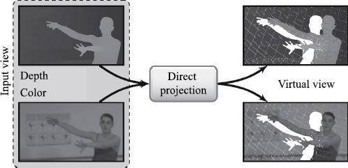
By applying this equation to each of the points in an acquired image, a new viewpoint can be generated. To do so, the information required includes the original image and its associated depth map as well as the camera parameters associated with the original and virtual viewpoints. This general principal of direct projection is illustrated in Figure 9.1.

9.2.1.2. Distortions associated with direct projection

Direct projection generates typical distortions found in viewpoint synthesis, i.e. uncovered zones, cracks and a ghost effect, as illustrated in Figure 9.2. The uncovered zones correspond to areas which are not visible from the original viewpoint and which become visible in the virtual image due to parallax. Cracks are tiny versions of these uncovered zones, principally due to resampling. Ghost contours are caused by projecting pixels whose color is a mixture of the background and foreground colors. Other typical distortions in viewpoint synthesis are caused by errors in the depth map produced within the estimation or compression stages. An error in the depth value creates a displacement in the point projected in the synthesized viewpoint. Resulting geometric deformations are typically texture stretches, deformed edges or isolated points (a crumbling effect).

9.2.1.3. Inverse projection

Figure 9.3 shows the general outline of inverse projection. Each pixel in the virtual viewpoint is retro-projected in the original viewpoint where its color is determined by interpolation. Retro-projection applies the transfer equation [9.4] from the virtual view to the original view using a depth map associated with the virtual view. This depth map must be estimated in advance using direct projection. Inverse projection is generally preferred to direct projection because it prevents distortions caused by resampling [MOR 09, NDJ 11, TSU 09]. Resampling distortions (such as cracks) and uncovered zones are present in the depth map estimated by direct projection but, given the typical appearance of a depth map (lack of texture, large uniform zones and soft variations), it is better to avoid and correct these distortions in the depth maps than to correct them in the synthesized viewpoints themselves.

9.2.2. Reducing distortions in viewpoint synthesis

Several methods have been proposed to prevent or correct synthesis distortions.

9.2.2.1. Cracks

Post-production can be used to suppress cracks while preserving contours. Nguyen et al. have proposed a bilateral color-depth filter to improve the estimated depth map by direct projection [NGU 09]. “Splatting” methods [RUS 00, PFI 00, ZWI 02] eliminate cracks. To reduce the algorithmic complexity in viewpoint synthesis, Zinger et al. [ZIN 10] have proposed applying inverse projection only to pixels labeled as cracks, i.e. those significantly modified by filtering. These cracks can also be treated via an evenly spaced ordering of projected pixels which will be described in section 9.2.2.3.

9.2.2.2. Ghost contours

Ghost contours are prevented by detecting discontinuities in depth (or overlap contours) in the depth map. The pixels near to these edges are projected during a secondary phase but only if they are visible, i.e. if their depth is inferior to that in the pixels projected previously [ZIT 04]. Müller et al. [MÜL 08] have proposed dividing the edge pixels into two classes: foreground edges and background edges. The pixels in this latter category are only projected if they fill empty zones. Ghost effects can also be avoided by evaluating the contribution of the background and foreground at the discontinuity edges using advanced background and foreground matting separation methods [CHU 02, HAS 06, WAN 07].

9.2.2.3. Uncovered areas

Uncovered areas are caused by unavailable information in the original image. Part of the uncovered area can be completed by information from other input viewpoints, if available, as is the case in viewpoint interpolation, examined in section 9.2.3. When information about the uncovered area is not present in any acquired image, a filling method is required. A low-pass depth image filter can be used to preprocess the image around the overlapping areas in order to limit gaps. Chen et al. [CHE 05] have also proposed a correction of vertical contours next to the edges in the depth map. These pretreatments are particularly well suited to small-scale uncovered areas. Large uncovered areas must be completed using texture “inpainting” methods which will be described in section 9.3.

However, in direct projection it is possible to propagate background values in the uncovered and cracked zones using a specific pixel order. The order proposed by McMillan [MCM 95] is based on epipolar geometry. This order applies the painting algorithm, i.e. it synthesizes the image first for the furthest points and then nearest points, with each new value potentially replacing a previously estimated value. As such, the uncovered areas are correctly treated with the visible point being the last to be examined. Uncovered zones and cracks can also be detected and treated using this ordering: if two successive points p and q in the path are projected onto the non-adjacent points p′ and q′, it is therefore a crack or an uncovered zone. The path order ensures that the first point p′ is in the background in relation to q′ and its value can be immediately propagated in the interval [p′,q′]. Jantet’s [JAN 12] Joint Projection Filling (JPF) algorithm distinguishes between cracks, where interpolation is carried out, and large uncovered zones where only the background value is propagated:

[9.5]

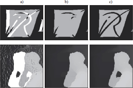
This method, which propagates or interpolates the background values at the point of projection, is well adapted for generating depth maps in direct projection, as shown in Figure 9.4.

9.2.3. Viewpoint interpolation

Viewpoint interpolation, introduced by Manning and Dyer [MAN 96], relates to synthesizing an intermediary viewpoint using several pieces of input data. Here, we consider input as view + depth (i.e. MVD, multi-view plus depth) data. The standard approach involves projecting two or three input views nearest to the virtual point and then fusing the obtained virtual viewpoints.

9.2.3.1. Fusing virtual viewpoints

The simplest fusion method is a linear combination, associated with a binary visibility map [CAR 03] or soft, i.e. non-binary visibility map [EIS 08]. The weighting factor is obtained using either the distance of input viewpoints from the virtual viewpoints or the relative angle of view between input viewpoints and the virtual viewpoints [BUE 01, DEB 96], or on the disparity using a different weighting for each point [DEV 11, TAN 08].

9.2.3.2. Detecting and smoothing distortions during interpolation

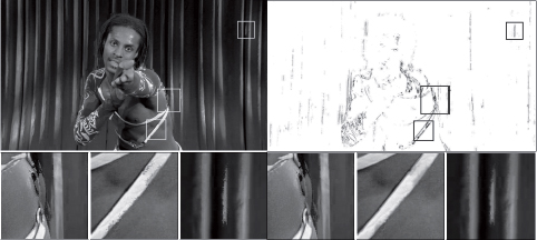
To limit the impact of geometric deformations due to errors in the depth map, several approaches have been proposed. Devernay et al. [DEV 11] have detected geometric distortions by comparing texture indices (intensity, gradient and Laplacian) at the point considered between the synthesized viewpoint and one of the original images. The idea is that the synthesized viewpoint must have the same kind of texture as the original viewpoints. A confidence map is then created and an anisotropic smoothing is applied to the low confidence zones, corresponding to strong differences in textures indices. The results obtained by this method are shown in Figure 9.5.

9.2.3.3. Floating textures

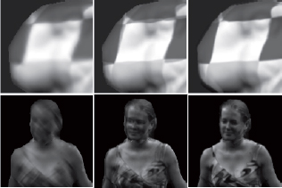
Depth errors and imprecision in the camera models and parameters cause geometric shifts during viewpoint synthesis. The linear combination of slightly offset textures produces a blurred effect. To avoid this, Eisemann et al. [EIS 08] have proposed the principle of floating textures. Synthesized viewpoints are readjusted, prior to linear combination, by estimation and dense motion compensation. A version which provides a quicker result applies an estimation/motion compensation to the original viewpoints and interpolates the motion fields obtained for the virtual viewpoint at the point of viewpoint synthesis.

9.2.3.4. Viewpoint extrapolation

Viewpoint extrapolation is the synthesis of a viewpoint outside the acquired viewpoint interval. When we only have a single input viewpoint, viewpoint synthesis is necessarily an extrapolation. This is also the case when we want to increase the interocular distance between images in a stereoscopic pair.

The main difficulty is therefore filling the uncovered zones because no original information is available. The methods cited previously are sufficient for small uncovered zones. When uncovered zones are larger, more complicated inpainting methods must be used to obtain a realistic effect.

9.3. Inpainting uncovered zones

As examined previously, the projection of a real viewpoint, also known as the reference viewpoint in another virtual camera referential, uncovers certain areas in the background. When the distance between the reference viewpoint and the virtual viewpoint becomes large, the uncovered zone increases in size and therefore becomes more difficult to fill. This problem is associated with both types of viewpoint synthesis methods, both interpolation and extrapolation methods. In order fill the background area, inpainting techniques are used. Before examining these methods, a few notations are necessary. Let us take an image I, defined by:

[9.6]

For color images, each pixel p is defined on three color planes (m = 3). The problem of inpainting in a viewpoint synthesis context can be formalized as follows: the image definition domain after projection is made up of two parts , with S being the known part (or source) of I and the unknown part U representing the uncovered zones. It is this part which we want to fill. In this section, we first provide a brief overview of 2D inpainting techniques. We then examine several extensions of 2D inpainting to 3D contexts.

9.3.1. Overview of 2D inpainting techniques

This section is not designed to be an exhaustive examination of current work in this field but to provide a general overview of the two main families of inpainting methods: diffusion-based methods and those based on searching for similarities using block (or patch) correspondences.

9.3.1.1. Diffusion-based methods

To fill the unknown zones in an image, one solution entails diffusing the information from the outside to the inside of the missing area. This type of approach, proposed by Bertalmio et al. [BER 00], uses the physical phenomenon of heat diffusion. The heat spreads until it reaches an equilibrium, i.e. a uniform distribution of temperature. By applying this phenomenon to reconstructing a missing zone in an image, it is possible to gradually spread the color information throughout the image. The diffusion procedure involves solving a partial derivative equation from the heat equation using an initial condition and Neumann limit conditions:

[9.7]

with div() being the divergence operators and f being a decreasing function of the gradient at the point p in the image I, noted as . This function affects the spread which can, for example, be linear isotropic, linear anisotropic or even nonlinear anisotropic.

These diffusion-based inpainting methods obtain very good results for filling uniform zones. However, they are not well adapted to textured images.

9.3.1.2. Similarity search based methods

More recent inpainting methods based on similarity searches can be summarized as five stages applied iteratively as follows:

Before discussing the mathematical purpose and details of these stages, a number of notations are required. A texture block centered on the point p is noted as . It is potentially composed of one part belonging to S and an unknown part belonging to U. Formally, the texture block can be written as: . The “filling property” p proposed in a precursor article [CRI 04] is designed to hierarchize filling to begin with the structure in the scene. Criminisi et al. have defined the priority P (p) at the point p as a product of two terms: a confidence term C(p) and a data term D(p). These terms are given by:

[9.8]

[9.9]

with in the patch area , with α being a normalization factor guaranteeing a dynamic between 0 and 1, n_p is the orthogonal unitary vector along the edge at the point p and is the gradient vector at the point p. Figure 9.7 shows the notations used in the previous formulas.

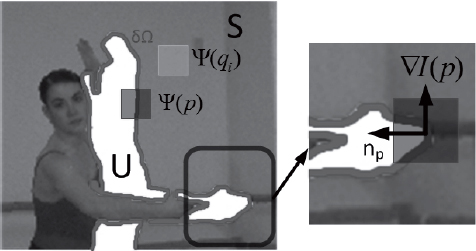
The term C(p), defined recursively (the term C(p) being initialized at 1 in the source region S), gives greater importance to the pixels p which are surrounded by known pixels. This term is the ratio between the numbers of known pixels compared to the total number of pixels in the block. The term D(p) attributes a strong importance to structured zones with an orthogonally oriented isophote along the edge (i.e. the boundary between S and U). The “similar block search” determines the most similar block in a local neighborhood, noted as , corresponding to the known part in the block :

[9.10]

with d(·) being the similarity metric. Often, we use the mean square error (MSE) calculated between the known pixels of the block considered and the candidate block. “Filling the unknown zone” of the block is achieved by recopying the co-localized pixels of the most similar block in the block .

There are a number of variations for these stages. For the filling priority, Le Meur et al. [LEM 11] have used a structure tensor to analyze the local geometry along the boundary line. For each point p, the structure tensor , spatially regularized by a Gaussian filter, is calculated as follows:

[9.11]

with I_i being the component i^nth of the image I, and Gσ being a Gaussian filter with a standard deviation of σ. The × operator is a matrix product and * represents the convolution operator. Analysis of the eigenvalues in the structure tensor λ_± determines the type of geometric structure. The orthogonal basis composed of the eigenvectors θ_± indicates the dominant orientations with θ_– being oriented in the direction of the isophote (parallel to the contour). When λ₊ is much greater than λ_–, the local geometric structure appears similar to a contour. This is illustrated in Figure 9.8 in the form of an ellipsis oriented in the direction of the contour (θ_–). A homogeneous zone is represented by highly similar values. It is represented by a circle, as illustrated in Figure 9.8. The use of a structure tensor increases resilience to noise and locates important structures in the scene better. In reference to work by [WEI 99], the term D(p) is written as:

[9.12]

with η being a positive constant value and α being a value between 0 and 1. When there is a strong structure (λ₊ >> λ_–), the term D(p) tends toward 1–α . If not, the term D(p) tends toward α. By choosing a low alpha value, a high value of the term D(p) indicates the presence of strongly structured zones. Another recent variation has been proposed by Xu et al. [XU 10]. In contrast to previous studies, Xu et al. [XU 10] have not used gradients to determine priority but the singular nature of the zone to be filled. The data term D(p) is calculated by measuring the redundancy of the known part in the block to be filled with its local neighborhood V. The term is defined by:

[9.13]

with being the norm L₂ and the vector w indicating the degrees of similarity between the known part of the block to be filled and the potential candidates , with . The similarity coefficient between the known part of the current block and a candidate block located at the point i is denoted by and is given by : , with and the term σ modulating the exponential decrease. To illustrate this method, we suppose that the vector w has a size of 4. For a block situated in a uniform zone, the similarity coefficients have a quasi-uniform distribution: , resulting in . However, if the block being filled shows a structure, the distribution of the coefficients is no longer uniform. For example, results in . The priority of this site is therefore superior to the previous site.

The second term of equation [9.13] weights the result according to the number of valid blocks (all the pixels in the block are known) and the total number of blocks N in the neighborhood .

In relation to the nearest neighbor search (stage 3 of inpainting, a variation of the algorithms based on a similarity search using block correspondences involves determining not only the best candidate but also the N best first candidates. These candidates are therefore combined linearly to obtain the value of the pixels in the unknown zone from the block to be filled :

[9.14]

with being the linear combination coefficients (respecting the constraint and the block centered on the point q_i being the most similar to the known zone of the current block centered on p. Here, the difficulty lies in determining the coefficients of the linear combination. There are several methods for doing this:

When the coefficients of the linear combination are determined, the unknown part of the block is synthesized via equation [9.14].

9.3.2. 3D Inpainting

9.3.2.1. An extension of Criminisi et al.’s approach to 3D contexts

The use of 2D inpainting algorithms in a 3D context is not necessarily easy. This is because the uncovered areas are most of the time close or connected to foreground areas. The aim of inpainting is to reconstruct these zones using information the background. This is a fundamental constraint since only background zones should be used when inpainting. Additionally, the foreground should not be propagated in the uncovered zone. Figure 9.9 illustrates this problem. The zones uncovered by projection (white areas in Figure 9.9(a)) are filled using Criminisi et al.’s method [CRI 04]. We can see that the background zones are recopied into the background, providing poor visual quality.

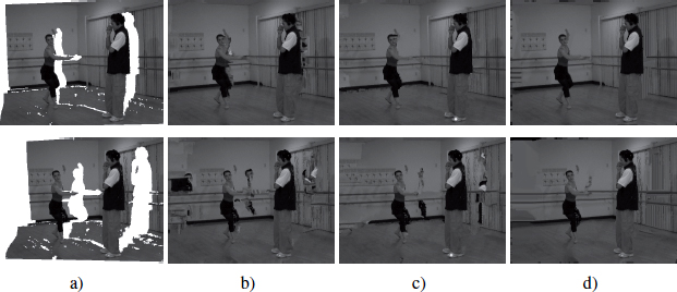
To solve such problems, Daribo and Pesquet-Popescu [DAR 10] suppose that the depth map is known and apply two modifications to the Criminisi algorithm. The first relates to calculating the priority P(p). In addition to the terms C(p) and D(p), Daribo and Pesquet-Popescu have integrated a term L(p) which is depth dependent:

[9.15]

with Z(p) being a block in the depth map z centered on the point p. L(p) is equal to 1 when the candidate is selected at the same depth as the block to be filled.

The second modification concerns the best candidate search which includes a depth term (with the notations of algorithm [9.10]) and a factor β in order to adjust the contribution of the second term as given below:

[9.16]

These two modifications restrict the filling procedure but do not necessarily remove the possibility of taking background blocks. The results of this approach are illustrated in Figure 9.9.

In 2011, Gautier et al. [GAU 11] extended the 2D approach by [LEM 11] to a 3D context. First, the term priority, which uses the structure tensor from the [LEM 11] method described in the previous section, is modified by adding the notion of depth. It is completed by a directional term which annuls the priority on part of the boundary line. The idea here is to consider the movement of the camera during viewpoint synthesis. A virtual viewpoint positioned to the right of the reference viewpoint requires a movement of the camera to the right. In this context, uncovered zones appear on the right of the foreground object. As a result, the order of filling must move from right to left (an illustration is shown in Figure 9.9). For a left camera movement, the order of filling is from left to right. This simple directional term effectively restricts filling in the uncovered zone. Thanks to this “trick” the foreground object can no longer be propagated in the background. These two modifications of the term priority and the candidate block search using depth, similarly carried out by [DAR 10], result in an improvement in quality, as shown in Figure 9.9. Note, however, that these two algorithms rely on the assumption that we know the depth map for the viewpoint in which the viewpoint references are projected.

9.3.2.2. Global optimization inpainting

Sun et al. [SUN 12] have filled uncovered zones with texture and depth while minimizing the overall energy defined in the unknown region U. The idea here is to determine the block belonging to the known region S which minimizes quadratic error in terms of texture and depth .It is defined by:

[9.17]

with I_o and Z_o being the reference viewpoint and its depth map, respectively. I and Z represent the synthesized viewpoint and its depth map. C represents the coordinates of the point where the energy is lowest. The first term represents the energy when the block centered on the point p is paired with a block in the known region S. The second represents the pairing of the block in terms of depth.

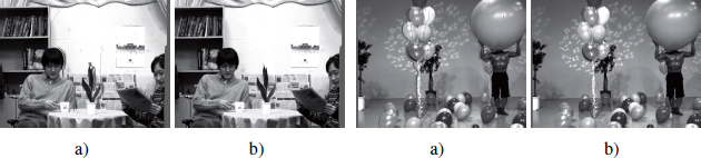
To infer the texture and depth of blocks in uncovered zones, Sun et al. used iterative Gauss–Seidel optimization by presupposing that either the depth or the texture of the block to be inpainted is successively known. Figure 9.10 shows the results of inpainting using this method, showing that the small uncovered areas are reconstructed well.

9.4. Conclusion

In this chapter, we have examined the problem of DIBR viewpoint synthesis using image plus depth information. A number of approaches have been proposed to avoid or limit problem distortions generated in the obtained virtual viewpoint, with the most difficult being the treatment of uncovered zones. The strategy which appears the most effective in this case is the combined used of information related to texture and depth. The evaluation of the quality of synthesized viewpoints remains an ongoing problem; on the one hand, we do not generally have a reference viewpoint and, on the other, existing quality measures (PSNR, SSIM, etc.) are not well suited to measuring the visual impact of geometric distortions and evaluating the visual quality of filling in an uncovered zone. However, the use of viewpoint synthesis to control view synthesis optimization quantification parameters has been recently proposed, normalizing the MVD data code, with a research group currently working on studying quality objective metrics in synthesizes viewpoints. If these studies are successful, they will open up new horizons for the use of viewpoint synthesis techniques to predict coding schemas in images and video.

9.5. Bibliography

[BER 00] BERTALMIO M., SAPIRO G., CASELLES V., et al., “Image inpainting”, Proceedings of SIGGRAPH 2000, 2000.

[BUA 05] BUADES A., COLL B., MOREL J., “A non local algorithm for image denoising”, IEEE Computer Vision and Pattern Recognition (CVPR), vol. 2, pp. 60–65, 2005.

[BUE 01] BUEHLER C., BOSSE M., MCMILLAN L., et al., “Unstructured lumigraph rendering”, in FIUME E., (ed.), SIGGRAPH 2001, Computer Graphics Proceedings, ACM Press/ACM SIGGRAPH, pp. 425–432, 2001.

[CAR 03] CARRANZA J., THEOBALT C., MAGNOR M.A., et al., “Free-viewpoint video of human actors”, ACM Transactions on Graphics, vol. 22, no. 3, pp. 569–577, 2003.

[CHE 05] CHEN W.-Y., CHANG Y.-L., LIN S.-F., et al., “Efficient depth image based rendering with edge dependent depth filter and interpolation”, ICME, pp. 1314–1317, 2005.

[CHU 02] CHUANG Y.-Y., AGARWALA A., CURLESS B., et al., “Video matting of complex scenes”, AACM Transactions on Graphics, vol. 21, no. 3, pp. 243–248, 2002.

[CRI 04] CRIMINISI A., PÉREZ P., TOYAMA K., “Region filling and object removal by examplar-based image inpainting”, IEEE Transactions on Image Processing, vol. 13, pp. 1200–1212, 2004.

[DAR 10] DARIBO I., PESQUET-POPESCU B., “Depth-aided image inpainting for novel view synthesis”, IEEE International Workshop on Multimedia Signal Processing, 2010.

[DEB 96] DEBEVEC P.E., TAYLOR C.J., MALIK J., “Modeling and rendering architecture from photographs: a hybrid geometry- and image-based approach”, SIGGRAPH ’96: Proceedings of the 23rd Annual Conference on Computer Graphics and Interactive Techniques ACM, New York, pp. 11–20, 1996.

[DEV 11] DEVERNAY F., DUCHÊNE S., RAMOS-PEON A., “Adapting stereoscopic movies to the viewing conditions using depth-preserving and artifact-free novel view synthesis”, in ANDREW J., WOODS N.S.H., DODGSON N.A., (eds), Proceedings of SPIE-IS&T Electronic Imaging, SDA 2011 – Stereoscopic Displays and Applications XXII, vol. 7863, SPIE and IST, San Francisco, CA, pp. 786302–786302, 12 March 2011.

[EIS 08] EISEMANN M., DECKER B.D., SELLENT A., et al., “Floating textures”, Computer Graphics Forum (Proceedings of the Eurographics EG’08), vol. 27, no. 2, pp. 409–418, 2008.

[FEH 04] FEHN C., “Depth-image-based rendering (DIBR), compression, and transmission for a new approach on 3D-TV”, SPIE 5291, Stereoscopic Displays and Virtual Reality Systems XI, pp. 93–104, 2004.

[GAU 11] GAUTIER J., LE MEUR O., GUILLEMOT C., “Depth-based image completion for view synthesis”, 3DTV Conference, 2011.

[HAS 06] HASINOFF S.W., KANG S.B., SZELISKI R., “Boundary matting for view synthesis”, Computer Vision and Image Understanding, vol. 103, no. 1, pp. 22–32, 2006.

[JAN 12] JANTET V., Layered depth images for multi-view video coding, PhD Thesis, University of Rennes, 1 November 2012.

[LEM 11] LE MEUR O., GAUTIER J., GUILLEMOT C., “Examplar-based inpainting based on local geometry”, ICIP, pp. 3401–3404, 2011.

[LIN 07] LIN C., “Projected gradient methods for non-negative matrix factorization”, Neural Computation, vol. 19, pp. 2756–2779, 2007.

[MAN 96] MANNING R.A., DYER C.R., “Dynamic view morphing”, Proceedings of the SIGGRAPH 96, pp. 21–30, 1996.

[MCM 95] MCMILLAN L., A list-priority rendering algorithm for redisplaying projected surfaces, Technical Report 95-005, University of North Carolina at Chapel Hill, NC, 1995.

[MOR 09] MORI Y., FUKUSHIMA N., YENDO T., et al., “View generation with 3D warping using depth information for FTV”, Signal Processing: Image Communication, vol. 24, nos. 1–2, pp. 65–72, 2009.

[MÜL 08] MÜLLER K., SMOLIC A., DIX K., et al., “View synthesis for advanced 3D video systems”, Eurasip Journal on Image and Video Processing - EURASIP J Image Video Process, vol. 2008, pp. 1–12, 2008.

[NDJ 11] NDJIKI-NYA P., KÖPPEL M., DOSHKOV D., et al., “Depth image-based rendering with advanced texture synthesis for 3-D video”, IEEE Transactions on Multimedia, vol. 13, no. 3, pp. 453–465, 2011.

[NGU 09] NGUYEN Q.H., DO M.N., PATEL S.J., “Depth image-based rendering with low resolution depth”, Image Processing (ICIP), 2009 16th IEEE International Conference on, pp. 553–556, 2009.

[PFI 00] PFISTER H., ZWICKER M., VAN BAAR J., et al., “Surfels: surface elements as rendering primitives”, SIGGRAPH ’00: Proceedings of the 27th Annual Conference on Computer Graphics and Interactive Techniques, ACM Press/Addison-Wesley Publishing Co., New York, pp. 335–342, 2000.

[ROW 00] ROWEIS S., SAUL L., “Nonlinear dimensionality reduction by locally linear embedding”, Science, vol. 290, pp. 2323–2326, 2000.

[RUS 00] RUSINKIEWICZ S., LEVOY M., “QSplat: a multiresolution point rendering system for large meshes”, SIGGRAPH ’00: Proceedings of the 27th Annual Conference on Computer Graphics and Interactive Techniques, ACM Press/Addison-Wesley Publishing Co., New York, pp. 343–352, 2000.

[SCH 05] SCHREER O., KAUFF P., SIKORA T., 3D Videocommunication: Algorithms, Concepts and Real-time Systems in Human Centred communication, John Wiley & Sons, 2005.

[SUN 12] SUN W., AU O.C., XU L., et al., “Texture optimization for seamless view synthesis through energy minimization”, ACM Multimedia, 2012.

[TAN 08] TANIMOTO M., FUJII T., SUZUKI K., et al., Reference Softwares for Depth Estimation and View Synthesis, ISO/IEC JTC1/SC29/WG11MPEG2008/M15377, April 2008.

[TSU 09] TSUNG P.-K., LIN P.-C., DING L.-F., et al., “Single iteration view interpolation for multiview video applications”, Proceedings of the 3DTV-Conference 2009, The True Vison, Capture, Transmission and Display of 3D Video, Postdam, Germany pp. 1–4, May 2009.

[WAN 07] WANG J., COHEN M.F., “Image and video matting: a survey”, Foundations and Trends in Computer Graphics and Vision, vol. 3, no. 2, pp. 97–175, 2007.

[WEI 99] WEICKERT J., “Coherence-enhancing diffusion filtering”, International Journal of Computer Vision, vol. 32, pp. 111–127, 1999.

[WON 06] WONG A., ORCHARD J., “A nonlocal-means approach to examplar-based inpainting”, Proceedings of the IEEE International Conference Image Processing (ICIP), pp. 2600–2603, 2006.

[XU 10] XU Z., SUN J., “Image inpainting by patch propagation using patch sparsity”, IEEE Transactions on Image Processing, vol. 19, no. 5, pp. 1153–1165, 2010.

[ZIN 10] ZINGER S., DO L., DE WITH P.H.N., “Free-viewpoint depth image based rendering”, Journal of Visual Communication and Image Representation, vol. 21, nos. 5–6, pp. 533–541, 2010.

[ZIT 04] ZITNICK C., KANG S., UYTTENDAELE M., et al., “High-quality video view interpolation using a layered representation”, ACM Transactions on Graphics, vol. 23, no. 3, pp. 600–608, 2004.

[ZWI 02] ZWICKER M., PFISTER H., VAN BAAR J., et al., “EWA splatting”, IEEE Transactions on Visualization and Computer Graphics, vol. 8, no. 3, pp. 223–238, 2002.

Chapter written by Luce MORIN, Olivier LE MEUR, Christine GUILLEMOT, Vincent JANTET and Josselin GAUTIER.