Chapter 2

Digital Cameras: Definitions and Principles

2.1. Introduction

Digital cameras are a common feature of most mobile phones. In this chapter, we will outline the fundamentals of digital cameras to help users understand the differences between image features formed by sensors and optics in order to control their governing parameters more accurately. We will examine a digital camera that captures not only still images but also video, given that most modern cameras are capable of capturing both types of image data.

This chapter provides a general overview of current camera components required in three-dimensional (3D) processing and labeling, which will be examined in the remainder of this book. We will study each stage of light transport via the camera’s optics, before light is captured as an image by the sensor and stored in a given format. Section 2.2 introduces the fundamentals of light transport as well as notations for wavelength and color spaces, commonly used in imaging. Section 2.3 examines how cameras have been adapted to capture and transform into digital image. This section also describes the details of different components in a camera and their influence on the final image. In particular, we will provide a brief overview of different optical components and sensors, examining their advantages and limitations. This section also explains how these limitations can be corrected by applying postprocessing algorithms to the acquired images. Section 2.4 investigates the link between camera models and the human visual system in terms of perception, optics and color fidelity. Section 2.5 briefly explores two current camera techniques: high-dynamic-range (HDR) and hyperspectral imaging.

2.2. Capturing light: physical fundamentals

Light enables humans to see their surrounding environments and capture it as images using cameras. The image obtained by a camera represents all the light rays reaching the camera’s sensors. To understand the basic concepts of this process, this chapter will examine the fundamentals of light transport. Section 2.2.1 examines generalized equations from radiometry and photometry and section 2.2.2 explains the influence of light wavelength. These aspects will be introduced due to their strong influence on digital imaging, image processing and image synthesis.

2.2.1. Radiometry and photometry

Radiometry quantitatively evaluates electromagnetic waves while photometry processes the sensation caused by this radiation for a standard observer [DEC 97]. Photometric values are obtained by combining radiometric values with the spectral response of this observer. The characteristic values of lighting and their photometric units are:

Luminous flux correspond to the light energy (number of photons) per time unit. They characterize the quantity of light radiation emitted by a source. Luminous intensity characterizes the flux emitted by a light source in a specific direction per unit solid angle:

[2.1]

Luminance characterizes the luminous flux per surface unit generated by a source with an intensity I at a distance d. It decreases according to the square of the distance:

[2.2]

where α is the angle between the normal of the lit surface and the direction of the source. Orders of the luminance value found in various lighting situations are presented in Table 2.1.

Table 2.1. Luminance produced by different light sources

Light source	Luminance (lux)
Full moon, cloudless sky	0.2
Movedto1m	1
Lit street	20 to 30
Dawn, dusk	50
Outside, cloudy weather	5,000
Sunny	10,000–20,000
Maximum measurable	100,000

Illuminance characterizes light intensity per unit surface in a specific direction. This is the most significant value for vision because it determines the visual sensation encountered by a user of the light being emitted, diffused or reflected according to the angle θ between the direction of emission ω_i and the angle of observation ω_o:

[2.3]

The bidirectional reflectance distribution function (BRDF), introduced by Nicodemus [NIC 67], describes the directional reflection of light by a surface element. It is defined as the relationship between the luminance reflected by the surface and the incident lighting. The integrated luminance L (ω_o) of an environment observed from the direction ω_o is given by the radiometric transfer equation [PER 88] – L becomes radiance when considering radiometry and wavelengths:

[2.4]

2.2.2. Wavelengths and color spaces

Electromagnetic radiation is represented as a continuous spectrum of wavelengths (see Figure 2.1). The human eye senses electromagnetic radiation with a wavelength approximately between 400 nm (upper threshold for ultraviolet light) and 700 nm (lower threshold for infrared light). White light is represented in appearance by a linear combination of three primaries, as demonstrated by Maxwell. Trivariance of a colored space was also established by Grassman. The three primary colors commonly used are red, green and blue (RGB). Metameric rays provide a colored image without having the same spectral content.

Colorimetry measures human perception of color and reduces the physical spectrum to the perceived color spectrum by correlation. It requires three essential elements: a light source (illuminantion), an object (with a standard measure of geometry) and a reference observer. In 1931, the International Commission on Illumination (Commission Internationale de l’Eclairage – CIE) carried out a series of psychophysical tests to deduce the standard colorimetric observation model that defines CIE 1931 color matching functions (CMFs) to quantify the perception of trichromatic color in human vision. In this experiment, two colors were shown to observers in normal colorimetric vision who should consolidate one of the stimuli with the appearance of the color. They used RGB lights to produce a metameric combination. The CMFs were then updated [STI 59, VOS 78]. These functions are official standards for the transformation of the visible spectrum to trichromatic color coordinates, CIEXYZ (the CIE tristimulus values). However, it was also found that the responses of the cones to long, middle and short (LMS) cones were different to physiological CMFs [EST 79, HUN 85]. A transformation of the cone’s response¹ proposed by Estévez [EST 79] is widely used in modern color appearance models.

A color space is a digital model of the human chromatic vision mechanism. The first trichromatic color model, CIEXYZ, was proposed in 1931 based on the red, green and blue colors. The correspondence between the CIEXYZ model established by the CIE and the cone model set out by Estévez is illustrated in Figure 2.1. However, the CIEXYZ model, while widely used, has a number of disadvantages, the first being that it is not physiologically but perceptually plausible. Added to this is the fact that this model’s representation gives negative values in relation to wavelength. These limitations have therefore led to research into other color appearance models.

Ideally, a color space is designed to represent perceived uniform colors in digital coordinates. Modern color spaces, often called color appearance models, are structured according to Zone theory [MUL 30], which describes human chromatic vision using a three-stage procedure. The calculation of color appearance includes chromatic adaptation, dynamic cone adaptation, decompositing opposite/achromatic colors and, in general, calculating perceptual color attributes. First, the input spectrum, sampled as tristimulus values XYZ, is transformed for chromatic adaptation often in relation to a specialized color space. The white adapted tristimulus values XYZ_c are then transformed in the cone color space where the cone response function is applied (often according to a power or hyperbolic function). The signal is then divided into achromatic channels A and opposite colors a and b. Finally, the perceptual correlation is based on these three channels. It is here that color perception models differ most because a large number of functions can be applied to produce these perceptual values. Popular models include CIELAB, RLAB [FAI 91], Hunt94 [HUN 94] and LLAB [LUO 96] and CIECAM97s [CIE 98], but CIECAM02 [MOR 02] has been commonly adopted as a standard appearance model.

The CIELAB color space [CIE 86] is very simple and based purely on the trichromatic component values XYZ. It is the oldest to be taken from the psychophysical approach in 1976. Chromatic adaptation is carried out by normalizing the values XYZ using the white reference values XYZ_w. This form modifies von Kries’ chromatic adaptation transformation [VON 70] and the cone response is modeled using a cubic root. Only lightness, chroma, hue and the color opponent coordinates (a and b) are predicted, and adaptation to different backgrounds or environments is not modeled. Despite these simplifications, the model performs well. The input parameters of the CIELAB model are the normalized CIEXYZ values (Y is equal to 100) of the test colors and the normalized values X_nY_nZ_n of the reference white.

The representation of colors in videos transmitted via television relies on the RGB model but relies on different transformation matrices to move from RGB to XYZ. This is confirmed by examples such as the National Television System Committee (NTSC) system used in the United States and Japan, the Phase Alternating Lines (PAL) system used by European countries such as the United Kingdom or Spain and the Sequentiel Couleur A Mémoire (SECAM – Sequential Color with Memory) system used in France, for example. Transmission takes place via signals, connected by transforming RGB components: Y, I, Q for NTSC; Y, U, V for PAL and Y, R-Y, B-Y for SECAM.

2.3. Digital camera

This section examines digital cameras and their diverse components. We will not attempt to provide an exhaustive overview of all possible configurations but purely the basic concepts necessary for understanding the choice of algorithms and the configurations of applications covered within this book.

2.3.1. Optical components

2.3.1.1. Optics in cameras

Electromagnetic radiation can be physically captured using optical mechanisms. The historical development of camera models has been examined in Chapter 1.

A camera is composed of a box and an objective lens. The objective lens contains several component lenses and a diaphragm that controls the transmission of light and is calibrated by an aperture unit (see section 2.3.3). This is represented by a number N that is defined as the focal length f of the lens divided by the diameter d of the pupil: N = f/d. For example, a lens with a pupil diameter of 25 mm and a focal length of 50 mm has a relative aperture of 50/25 = 2.0. The diaphragm is expressed according to the focal distance f and is described in italics, for example, by f/4 when the relative aperture N has a value of 4. The denominator of the expression is generally indicated by the f-number of the lens and the relative aperture simply as its aperture or f-stop. If there are two apertures and aperture speed configurations, they satisfy the following relation: [RAY 00] because the amount of energy received by the sensor is proportional to the diaphragm’s free surface and therefore the square of the aperture.

2.3.1.2. Errors and corrections

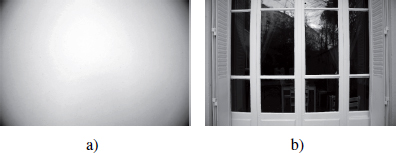
The mechanical and optical geometry of a camera may result in deformation and undesired effects in the image. For example, the reception of light by sensors will be much higher at the center of the image than at the edges. This effect is known as fall-off or vignetting and is illustrated in Figure 2.2(a), for an image acquired with a bigger aperture (which accentuates the effect). Also evident is the distortion of the image due to the lens (see Figure 2.2(b)). Another effect of light reflection is known as flare, which produces color effects that do not exist in real life. This is due to the multiple reflection of light onto the lenses in question. These three effects can be compensated for using automatic algorithms (see Chapter 5) precisely so that they can be measured. For example, a photograph of a white wall can be used to measure the effect of fall-off and a generic correction in cos⁴ can be applied. In addition, a correction of radial distortion can be applied to the image but this creates an image that is no longer rectangular. Algorithms to counter flare have also been proposed, specifically by Ward [REI 10].

Filters can be directly applied to camera lenses. Neutral density filters attenuate light according to a relation producing an effect similar to a decrease in exposure time. They are used, for example, to create an effect of movement by increasing the exposure time while maintaining adapted light intensity values. Polarizing filters (circular or linear) block specific light rays. They are mobile, which means that specific desired effects can be chosen. In particular, reflective effects can be attenuated or the color contrast can be augmented.

2.3.2. Electrical components

The sensor in a camera has the primary function of converting light signals into electronic signals. Current cameras are generally fitted with an image sensor based on charged coupled device (CCD) technology or a complementary metal oxide semiconductor (CMOS). Either a charge coupled device (CCD) or a complementary metal oxide semiconductor (CMOS) are commonly employed as imaging sensors in current cameras. Nowadays the CCD sensors are preferred in high-end applications due to better performance with less noise, while the CMOS sensors are popularly used in commodity camera systems.

The CCD sensor system has been used in cameras for more than 20 years. Due to the smaller size of the light collecting area, light sensitivity of the CMOS is lower than that of the CCD in general. CCD sensors are, however, more costly due to the non-standard manufacturing process used to manufacture them. In addition, a phenomenon known as blooming is likely to occur when a very bright object (for example a lamp or sunlight) is present in a scene. This can produce vertical lines above and below the object.

Due to the cost of CCD sensors, CMOS sensors have been subject to a number of improvements. It is thus difficult to identify which sensor obtains the best quality. CMOS sensors reduce the overall cost of the camera because they integrate several necessary elements. They can also be used to produce small-scale cameras. One of the current limits of CMOS sensors relates to their low sensitivity to light. If the problem does not arise in normal lighting conditions, it can occur as luminance decreases. The resulting image is therefore either very dark or blurred (noise).

Two types of noise occur depending on the sensor system used: temporal noise, which varies according to each picture, and fixed noise, associated with sensor irregularities. The different types of noise are well known and there are several methods of measurement and corrections. In fact, several noises have already been compensated for by manufacturers using hardware and/or software components. The easiest noise to correct is thermal noise, which can be due to both noise on the sensors and noise due to agitated electrons, varying according to temperature. It can be measured by taking a photograph with a hood over the object in order to block light. The acquired pixels do not represent a true black while no light reaches the sensors. This noise can often be corrected by approximation by subtracting the average value obtained for this or these black image(s) from the image pixels acquired in normal conditions.

2.3.3. Principal functions and their control

Manual mode requires the selection of parameters such as focus, gain white balance, exposure time and the diaphragm aperture, whose values are best selected in the automatic mode.

Change of focus affects the sharpness of the image. A change in focus value will modify the position of the lens inside the objective and therefore the trajectory of light toward the sensors according to the laws of physics. The divergence or convergence of emitted light rays defines the blurred or sharp parts of the image.

As explained in section 2.3.1.1, the diaphragm’s aperture is generally associated with the f-stop value N, corresponding to the relation between focal distance and the diaphragm’s diameter. The smaller the f-stop, the wider the diaphragm aperture. It is characterized by values such as f/2 for a very wide aperture and f/22 for a very small aperture. The gap between f-stops is often calculated by dividing by a power of The diaphragm aperture affects the larger or smaller passage of light. This has a strong effect on depth of field: the wider the aperture (small f-stop value) is, the more the depth of field is reduced. A reduced depth of field highlights a subject and blurs the background and foreground while a higher depth of field sharpens details in the image.

Exposure time t is measured in seconds, often with a relation of 2 between two exposure times such as the times 1/16 and 1/32 s. It refers to the duration of the shutter’s opening. The longer the exposure time, the more light the sensors will collect. A long exposure time therefore provides a bright image while a short exposure time leads to a dark image. The exposure time and aperture f-stop are connected by an exposure value (EV):

[2.5]

In photography, f-stop is often confused with stop, which is a relation. Stop can be used in relation to different EV values: a variation of 1 (relation of 2 on the exposure time) on an EV will give a 1 stop unit. The term “stop” is also used to size an intensity interval: n stops corresponding to a size of 2ⁿ.

Sensor gain affects the light intensity values that can be obtained. It relates to the sensitivity of the film to light. With digital devices, this property does not exist any more since there is no longer a film. It is now related to the gain applied to the sensor signal. The higher its values are, the more the acquisition is light sensitive. For a number of photographic devices, this is accompanied by noise on the image for higher ISO values.

Lastly, the white balance reflects the color measured in Kelvins (K). The eye adapts its perception of white. If the image’s color is not calibrated, the resulting image can differ, which is directly evident. A poor choice of white balance will provide an image that seems yellow (warm tones) or lacking in color (cold tones).

A number of cameras are fitted with a bracketing function, which allows photographs to be taken according to several device parameters. It is used primarily for white balance as well as exposure. It is possible to take a sequence of images in the automatic mode, which will vary one parameter while the others remain fixed. This bracketing mode does not have an equivalent in video cameras although some recording techniques have proposed alternatives (see Chapter 19).

We will examine the bracketing function applied to varying exposure time for a single aperture. This is useful for understanding Chapter 19 of this book. This bracketing mode on exposure time is based on three hypotheses: a number n (odd) images (often from three to nine depending on the camera), an aperture diaphragm with a value of N and a fixed ratio r. Generally, the camera selects the most appropriate exposure time t₀ for the content whose related EV linking N to t₀ is indicated by the symbol EV₀, producing an intermediary photograph. A series of n photographs are taken with the diaphragm aperture N with the relative EVs: EV_–n/2, EV_–(n–2)/2, ..., EV₀, ..., EV_(n–2)/2, EV_n/2. For example, the exposure time used for the image acquired in EV_–n/2 is t₀/r(n/2). This provides a burst of a series of images of the same scene but representing different levels of brightness.

2.3.4. Storage formats for images

In low dynamic imaging, the most current format encodes photometric data using the three red, yellow and blue channels, which correspond to the dominant colors of the three ranges of wavelength that they represent. These channels are encoded using an 8-bit integer defining 256 levels for each one. However, color encoding according to the RGB addition principle cannot satisfy all applications (notably in image processing) and other color representation spaces exist to adapt it, notably the CIEXYZ format examined in section 2.2.2.

Image formats differ according to two aspects: the color representation range (which can go beyond the 8 standard bits), the compression and decompression mechanisms, and the type of compression (with or without loss). There are several types of standard, with the information loss compression formats including: Joint Photographic Experts Group (JPEG), Tagged Image File Format (TIFF), and lossless formats including: Graphics Interchange Format (GIF) and Portable Network Graphics (PNG). The majority of cameras can store images in RAW format, which is not a standard format. Each manufacturer defines its RAW format (with an appropriate extension), which must be coded differently. The RAW format encodes a multitude of different pieces of information as well as pixels’ color values, in the form of metadata, which can be formalized in Exchangeable image file format (EXIF). This format, proposed initially by the Japan Electronic Industries Development Association (JEIDA), has been adopted by the majority of manufacturers. Information related to camera parameters at the point of image capture and the size and resolution of the image often constitutes part of this. Colors are represented in mosaic form using a Bayer filter (1976) or a color-filter-array such as those filtered directly by sensors. They are represented by 50% green, 25% blue and 25% red, or a format known as RGGB. When constructed, the image must be “debayerized” or subject to “demosaicing”, for which there are a number of methods [LI 08]. While sometimes compressed, the RAW format can, in theory, provide access to data acquired by sensors.

2.4. Cameras, human vision and color

Human perception is examined in Chapters 1 and 16 in relation to pinhole cameras. In this chapter, however, we will examine the relationship between human perception and cameras.

2.4.1. Adapting optics and electronics to human perception

The human visual system is widely used to evaluate display devices [BRE 10]. However, it is rarely used to design and evaluate digital cameras, specifically their sensors, despite the fact that they are fundamental systems within an image capturing device. Equally, while the aim is that sensors must generally exceed the human eye, there is currently no means of measuring the gap between a sensor and the human visual system.

To overcome this issue, Skorka and Joseph [SKO 11] recently introduced a performance evaluation method for digital cameras in relation to the human visual system. They selected eight parameters to characterize an imaging system. The system implemented is conveyed by a quality factor that represents the gap in performance for the parameter that appears the weakest when compared to the human eye. For each of these eight parameters, an ad hoc evaluation method is proposed. The different parameters considered include energy consumption, visual field, spatial resolution, temporal resolution, the peak signal-to-noise ratio (PSNR) and the dynamic and obscurity current. Data related to the human visual system were collected from clinical or psychophysical data collected in the literature while data regarding sensors were gathered from manufacturers’ own data. They applied their method to 24 modern CCD or CMOS sensors (either academic or commercial) proposing an ideal lens each time to form a complete imaging system. In the majority of cases, dynamic proved to be the most limiting factor in relation to the human visual system, followed by the dark current. Overall, the evaluation showed that modern digital cameras are not yet able to rival the human eye. The estimated gap lies between 31 and 90 dB, with an order ranging between 1.6 and 4.5.

2.4.2. Controlling color

2.4.2.1. Response functions in cameras

The image acquired by the camera differs strongly from the real scene in terms of color. The choice of constructor in the sensor response has a strong influence on the final luminance. Each camera generally has its own response function that converts the radiance values into color values to be allocated to pixels. To revert to radiance values, it is necessary to estimate the inverse response function. If we consider the irradiance E reaching the camera’s sensor, there is a linear relation with the scene’s irradiance, generally depending on the exposure time t. The intensity value M stored in the image corresponds to the conversion t, such that M = f(E). Its inverse function is used to obtain the radiance. Generally, this process involves selecting the value of identical pixels for different exposure times in order to monitor the variation in their intensity to adjust the best curve separately for each R, G and B channel. Several methods for estimating this function exist in the literature, which generally consider f as a monotonic and increasing function, thereby ensuring that it is invertible. Additional hypotheses can be proposed in relation to its form: logarithmic [DEB 97], polynomial [MIT 99] or gamma [MAN 95]. A function can also be reconstructed using other known functions [GRO 04]. However, the procedure is very sensitive to the pixels selected and the input images. If the camera’s parameters are unchanged, we can use the same curve for other images.

2.4.2.2. Characterizing color

If optical radiation in a reference test chart is measured and sensed simultaneously by a detection device in an image, it is possible to create a mathematical model to describe the specification of the color of an image device in coordinates with a physical meaning that is independent of the device. The device’s signals or the images’ colors vary according to the manufacturer’s specifications or the material used. They can also vary when there are identical specifications due to the manufacturing process. The characterization of colors exceeds the variation in image devices by constructing a mathematical bridge between the device signal and the physical coordinates such that we can describe the device-dependent signals as independent signals. For example, CIEXYZ or CIELAB can be used as independent signals. To do so, it is necessary to use measuring tools for physical properties or produced desired colors in the output device. The characterization of colors requires a two-stage procedure [JOH 02]. The first is calibration, which is the setting up of a device or process so that the device gives repeatable data. The following stage is characterization, which establishes a relationship between the device’s color space and the independent color space such as the CIE tristimulus values. Further information regarding this will follow in Chapter 5.

2.5. Improving current performance

Over the past 10 years, digital imaging technology has exploded. New horizons are continually opening up and research is focusing on a number of complementary domains that will converge in the near future. In this book, we can specifically cite stereoscopic photography, HDR imaging and multispectral acquisition. Here, we will concentrate on the two latter examples, given that the former will be examined in Chapter 3.

2.5.1. HDR imaging

Today, classic images are referred to as low-dynamic-range (LDR) images. These are images whose colors are typically represented by an interval of 8 bits. In contrast, we also have images known as HDR images, which go beyond this reduced representation. There is currently no precise consensus around the exact definition of HDR images. If we consider full HDR, this entails reconstituting the existing intensities in a given scene and storing them as an image or video. On the basis of 16 stops, all intensities are represented for a wide range of scenes. The popularity of these images is undeniable and even precedes the progression and development of the field. Photographic sensors can now cover a dynamic storable range of up to 16 or even 20 bits (the camera created by Spheron²) although in a 1D sequential acquisition. Video sensors are generally more limited to 12 bits and a maximum of 14 bits, with the exception of 20 bits in Spheron’s experimental video camera.

Different methods have been developed to reproduce HDR content using a spectrum provided by current sensors but have faced a number of more significant obstacles with regard to producing videos. They are principally created by combining images taken with different exposure times. The bracketing mode (see section 2.3.3) is particularly useful. Nearly all approaches, software and materials rely on this approach. A model of optical reconstruction and its sensors is essential for the quality of obtained images [AGU 12]. The use of RAW format (see section 2.3.4) allows us to avoid the need of camera functions (see section 2.4.2.1) and is thus preferable. The initial HDR photograph creation approaches for static scenes examined in [BAN 11, REI 10] and applied to different commercial software can be differentiated from more recent approaches, which use dynamic contexts and video data as explained in Chapter 19.

Storing a range of HDR radiance values is subject to specific coding. Colors can be stored at 32 bits (compared to 24 bits for LDR images). Different HDR formats are generally inspired by the LDR formats (see section 2.3.4). The RGBE format [WAR 91] is an extended version of sRBG (RGB including a gamma correction normalized between 0 and 1) to which an E channel is added corresponding to the exponent to a power of 2 that is applied to the RGB values, which gives their high dynamic equivalent. From this format, we can derive an XYZE format that extends the CIEXYZ norm to HDR images. The corresponding extension of this image format is .hdr. Another available HDR format is known as LogLuv TIFF. It is inspired by the CIELUV format and encoded the L component (radiance) logarithmically [WAR 98]. However, this coding results in a greater amount of information loss than XYZE for an equivalent memory use (for a comparison of different formats, see [REI 10]). Lastly, the OpenEXR format directly encodes the RGB channels onto three floats, with 96 bits per pixel (format considered to be lossless or half-float (16 bits per component or 48 bits per pixel)) [KAI 09].

2.5.2. Hyperspectral acquisition

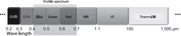
Electromagnetic radiation is generally described in terms of photon wavelength. Spectral intervals are classified according to three categories: near-ultraviolet (NUV) 300–400 nm, visible (VIS) 400–700 nm, and near-infrared (NIR) 700 nm–3.0 μm [ISO 07]. Trichromatic imaging and multispectral imaging focus on the VIS category while hyperspectral imaging (see Figure 2.3) focuses on three categories (NUV, VIS and NIR). Spectral imagery can be categorized according to different concepts, i.e., by filter of monochromatic sensor.

Several filter-based concepts have been proposed. When a complete spectrum light source shines on the surface of an object, the light reflected is captured by an extended bandwidth filter device [ATT 03, RAP 05, WAR 00]. These filters, fitted in a motorized wheel or a tunable liquid crystal filter (LCTF), are used to identify the spectrum in question. An alternative to the bandwidth filter is a spectral dispersion unit. Spectral images are reconstructed by a reverse solution, producing artifacts and a spatial resolution inferior to the bandwidth in question [KIT 10].

A monochromatic sensor captures the surface of an object receiving light within a narrow bandwidth [EAS 10, FRA 10, KIM 10]. This method does not light the object with a complete spectrum light source such as a xenon light, thereby minimizing ionization damage. Because of the evolution of Light-Emitting Diode (LED) technology, the configuration of narrow bandwidth LED lights will be more effective in terms of cost than a complete spectrum light. Fluorescence (emission of light by a substance absorbing light of different wavelengths such as NUV) forms part of the reflected light and thereby interferes in measures of reflectance for each wavelength.

2.6. Conclusion

In this chapter, we have studied the fundamental of image acquisition. We have examined camera technology in relation to the transport of light since photographic sensors receive light rays that have traveled through the camera lens and diaphragm. We have also explained the image capture mechanism through various optical and electronic components and the relationship of different parameters with the final image obtained. Current technology is not free from faults, which may induce geometric or colorimetric deformations. We have explained these limitations in relation to current solutions to them. Further details on this subject are examined by Reinhard et al. in [REI 08], which provide a number of details regarding image acquisition and color. A number of points examined briefly in this chapter will be discussed in depth in following chapters.

2.7. Bibliography

[AGU 12] AGUERREBERE C., DELON J., GOUSSEAU Y. et al., Study of the digital camera acquisition process and statistical modeling of the sensor raw data, Report Instituto de Ingenieria Eléctrica (IIE), Paris, September 2012.

[ATT 03] ATTAS M., CLOUTIS E., COLLINS C., et al., “Near-infrared spectroscopic imaging in art conservation: investigation of drawing constituents”, Journal of Cultural Heritage, vol. 4, pp. 127–136, 2003.

[BAN 11] BANTERLE F., ARTUSI A., DEBATTISTA K. et al., Advanced High Dynamic Range Imaging: Theory and Practice, AK Peters (CRC Press), Natick, MA, 2011.

[BRE 10] BREMOND R., TAREL J.-P., DUMONT E. et al., “Vision models for image quality assessment: one is not enough”, Journal of Electronic Imaging, vol. 19, no. 4, pp. 1–14, 2010.

[CIE 86] CIE, Colorimetry, CIE Pub. no. 15.2, Commission Internationale de l’Eclairage (CIE), Vienna, 1986.

[CIE 98] CIE, The CIE 1997 interim colour appearance model (Simple Version), CIECAM97s, CIE Pub. no. 131, Commission Internationale de l’Eclairage (CIE), Vienna, 1998.

[DEB 97] DEBEVEC P.E., MALIK J., “Recovering high dynamic range radiance maps from photographs”, Proceedings of ACM Siggraph ’97 (Computer Graphics), ACM, pp. 369–378, 1997.

[DEC 97] DECUSATIS C., (ed.), Handbook of Applied Photometry, AIP Press, Springer, 1997.

[EAS 10] EASTON R., KNOX K., CHRISTENS-BARRY W., et al., “Standardized system for multispectral imaging of palimpsests”, Proceedings of the SPIE, Computer Vision and Image Analysis of Art, SPIE, no. 75310D, pp. 1–11, 2010.

[EST 79] ESTÉVEZ O., On the fundamental data-base of normal and dichromatic colour vision, PhD Thesis, University of Amsterdam, 1979.

[FAI 91] FAIRCHILD M. D., “Formulation and testing of an incomplete-chromatic adaptation model”, Color Research and Application, vol. 16, no. 4, pp. 243–250, 1991.

[FRA 10] FRANCE F. G., CHRISTENS-BARRY W., TOTH M. B. et al., “Advanced image analysis for the preservation of cultural heritage”, IS&T/SPIE Electronic Imaging. International Society for Optics and Photonics, SPIE, no. 75310E, pp. 1–11, 2010.

[GRO 04] GROSSBERG M.D., NAYAR S .K., “Modeling the space of camera response functions”, IEEE Transactions on Pattern Analysis Machine Intelligence, vol. 26, no. 10, pp. 1272–1282, October, 2004.

[HUN 85] HUNT R.W.G., POINTER M.R., “A colour-appearance transform for the CIE 1931 standard colorimetric observer”, Color Research and Application, vol. 10, no. 3, pp. 165–179, 1985.

[HUN 94] HUNT R.W.G., “An improved predictor of colourfulness in a model of colour vision”, Color Research and Application, vol. 19, no. 1, pp. 23–26, 1994.

[ISO 07] ISO, ISO/20473:2007: Optics and Photonics — Spectral Bands, 2007.

[JOH 02] JOHNSON T., “Methods for characterizing colour scanners and digital cameras”, in GREEN P., MACDONALD L.W., (eds), Colour Engineering, Achieving Device, Independent Colour, John Wiley & Sons Inc., Chichester, pp. 165–178, 2002.

[KAI 09] KAINZ F., BOGART R., “Technical introduction to OpenEXR”, 2009. Available at http://www.openexr.com/index.html.

[KIM 10] KIM S.J., ZHUO S., DENG F., et al., “Interactive visualization of hyperspectral images of historical documents”, IEEE Transactions on Visualization and Computer Graphics, vol. 16, no. 6, pp. 1441–1448, 2010.

[KIT 10] KITTLE D., CHOI K., WAGADARIKAR A. et al., “Multiframe image estimation for coded aperture snapshot spectral imagers”, Applied Optics Opt., vol. 49, no. 36, pp. 6824–6833, 2010.

[LI 08] LI X., GUNTURK B., ZHANG L., “Image demosaicing: a systematic survey” Visual Communications and Image Processing 2008, Proceedings of the SPIE, pp. 68221J–68221J–15, 2008.

[LUO 96] LUO M.R., LO M.-C., KUO W.-G., “The LLAB (l:c) colour model”, Color Research and Application, vol. 21, no. 6, pp. 412–429, 1996.

[MAN 95] MANN S., PICARD R.W., “Being undigital with digital cameras: extending dynamic range by combining differently exposed pictures”, Proceedings of IST 46th Annual Conference, Boston, Massachusetts, pp. 422–428, May 1994.

[MIT 99] MITSUNAGA T., NAYAR S. K., “Radiometric self calibration”, Proceedings of IEEE Conference on Computer Vision and Pattern Recognition, Fort Collins, CO, pp. 374–380, June 1999.

[MOR 02] MORONEY N., FAIRCHILD M.D., HUNT R.W.G., et al., “The CIECAM02 color appearance model”, Proceedings of the 10th IS&T Color Imaging Conference, IS&T, pp. 23–27, 2002.

[MUL 30] MULLER G.E., “Über die Farbenempfindungen”, Z. Psychol., pp. Erganzungsbände 17 and 18, 1930.

[NIC 67] NICODEMUS F.E., “Radiometry”, Applied Optics and Optical Engineering, vol. IV, Academic Press, New York, 1967.

[PER 88] PÉROCHE B., La Synthèse d’Images, Hermès Science Publications, 1988.

[RAP 05] RAPANTZIKOS K., BALAS C., “Hyperspectral imaging: potential in non-destructive analysis of palimpsests”, Proceedings of the 2005 International Conference on Image Processing, ICIP 2005, vol. 2, pp. II, 618–21, September 2005.

[RAY 00] RAY S.F., “The Geometry of image formation”, in JACOBSON R., RAY S., ATTRIDGE G.G., AXFORD N. (eds), The Manual of Photography, 9th ed., Focal Press, Oxford, pp. 39–71, 2000.

[REI 08] REINHARD E., KHAN E.A., AKYZ A.O., et al., Color Imaging: Fundamentals and Applications, AK Peters, Ltd., 2008.

[REI 10] REINHARD E., WARD G., PATTANAIK S., et al., High Dynamic Range Imaging: Acquisition, Display, and Image-based Lighting, 2nd ed. The Morgan Kaufmann series in Computer Graphics, Elsevier (Morgan Kaufmann), Burlington, MA, 2010.

[SKO 11] SKORKA O., JOSEPH D., “Toward a digital camera to rival the human eye”, Journal of Electronic Imaging, vol. 20, no. 3, pp. 1–18, 2011.

[STI 59] STILES W.S., BURCH J.M., “NPL colour-matching investigation: final report”, Optica Acta, vol. 6, pp. 1–26, 1959.

[VON 70] VON KRIES J., “Chromatic adaptation”, in MACADAM D.L., (ed.), Sources of Color Science, MIT Press, Cambridge, pp. 109–119, 1970.

[VOS 78] VOS J.J., “Colorimetric and photometric properties of a 2-deg fundamental observer”, Color Research and Application, vol. 3, pp. 125–128, 1978.

[WAR 91] WARD G., “The LogLuv encoding for full gamut, high dynamic range images”, in ARVO J., Ed., Graphics Gems II, Academic Press Inc., pp. 80–83, 1991.

[WAR 98] WARD G., “The LogLuv encoding for full gamut, high dynamic range images”, Journal of Graphics Tools, vol. 3, no. 1, pp. 15–31, 1998.

[WAR 00] WARE G.A., CHABRIES D.M., CHRISTIANSEN R.W., et al., “Multispectral analysis of ancient Maya pigments: implications for the Naj Tunich Corpus”, IEEE Transactions, pp. 2489–2491, 2000.

1 Photoreceptors in the eye convert electromagnetic signals from light into nerve signals.

2 www.spheron.fr/.

Chapter written by Min H. KIM, Nicolas HAUTIÈRE and Céline LOSCOS.