
Chapter 7
Confidence Limits and Hypothesis Testing
One of the most important functions of statistics, and the one to which the remainder of this book is devoted, is the determination of whether two variables could be considered to be independent of each other. This is a determination that is made on a sample of observations but is understood to apply to an entire population. The central task of determining independence is the establishment of confidence limits and the testing of hypotheses about the data.
7.1 What Is a Confidence Interval?
A confidence interval is the range within which we expect a true population value (e.g., a mean) to lie.
A confidence interval is the range within which we expect a true population value (e.g., a mean) to lie. Confidence intervals are established from samples and are used to predict a population value when it is not possible (e.g., because of high cost or limited time) to measure the true value directly. For example, suppose a hospital financial officer wishes to know the average cost of services provided to the hospital's inpatients. But the only record that the hospital maintains for most hospital stays is information about the insurance-reimbursable amount and total charges. Both of these items are based primarily on length of stay and diagnosis. The only way to get the actual cost of services for any inpatient stay is to examine the specific hospital record, determine which services were provided, and assign a cost to each of these services. In addition, an average-sized hospital might have 10,000 to 15,000 discharges in a given year. If the financial officer were to try to examine each of these to determine the average cost of services provided to inpatients, the magnitude of the task would be prohibitive.
Using a Representative Sample to Infer a Mean
So what is that financial officer to do? The financial officer might reasonably expect that such an assessment could be made for a sample of hospital discharges (e.g., 100). Let's say the financial officer selected a random sample of 100 hospital discharges from all discharges for the past year. It could then be possible to estimate, on the basis of this sample, the true mean cost of services for inpatients. In doing this, the financial officer would calculate a mean value for the sample and infer that this is the mean for all discharges. But as we saw in Chapter 6, the mean value for one sample would not necessarily be the same as the mean value of a second sample. In fact, we learned that if we selected many samples, the means from those many samples would tend to be normally distributed around the mean of all samples (and also around the true mean of all discharges).
Now, the financial officer should be very interested in this point estimate (i.e., the sample mean) of costs per discharge. However, he might also be interested in the range within which the true population mean of costs for all discharges might lie if he were able to measure the cost of all discharges. To examine this question, he would have to begin integrating the mean with a measure of dispersion. To do this we need to return to the data from the 12,000 hospital discharges examined in Chapter 6. But this time, instead of looking at length of stay, we are going to look at hospital costs. In turn, we must look at both a point estimate of the sample mean and the dispersion around that mean to create a confidence interval. How to get from point estimates to confidence intervals is discussed next.
From Point Estimates to Confidence Intervals
As was previously discussed, it is infeasible for the hospital financial officer to get the true mean cost of discharges for the year. However, for the sake of discussion in this book, let us assume that we have accomplished this and that the mean cost of a discharge is $5,905.75. The distribution of costs in standard deviation units is shown in Figure 7.1. Column A shows standard deviation units above and below the actual mean of $5,905.75. Column B shows the actual dollar amount at the top of each standard deviation range. Column C shows the proportion of discharges in the range up to the dollar amount shown in column B. For example, the value $5,905.75 in column B represents those discharges that cost between $1,125.29 and $5,905.75. All other cells in column B are interpreted similarly.

Figure 7.1 Distribution of costs for 12,000 discharges
It appears, then, from Figure 7.1, that just over 65 percent of all hospital discharges have costs in the range of 1 standard deviation below the mean (those in cell C4). Twenty-three percent of all discharges have costs in the range of 1 standard deviation above the mean (those in cell C5). Only 0.8 percent of discharges have costs below 1 standard deviation below the mean (cell C3). The remaining discharges have costs ranging from 1 standard deviation above the mean to 9 standard deviations above the mean. Clearly, actual costs are not normally distributed. However, based on what was learned in Chapter 6, we can have some confidence that if samples of a large enough size are taken, the means of those samples will be approximately normally distributed. This assumption is valid in that it is the mean that we wish to estimate rather than any one individual discharge cost.
Integrating the Sample Mean and Standard Error
So, for example, suppose the financial officer chose a random sample of 100 discharges from among all the hospital discharges for the year in question. In turn, let's say he determined after an examination of the records that the mean for the 100 discharges was exactly $6,586.30. He might then infer that the true average cost of hospital stays was $6,586.30. However, the financial officer must keep in mind that this is only an estimate about the population mean based on a sample.
Now, because the officer had a graduate course in statistics he decides to determine a confidence interval for this mean value. The financial officer remembers that sample mean values are distributed approximately as a t distribution, with degrees of freedom (df) equal to the sample size minus 1—for our example, ![]() . He also remembers that having two standard errors on either side of the mean gives the approximate range in which he will have a 95 percent likelihood of finding the true mean of the population. (In fact, 1.98 standard deviations on either side of the mean will give him the exact 95 percent likelihood of finding the true mean, but 2 is close enough in most applications.)
. He also remembers that having two standard errors on either side of the mean gives the approximate range in which he will have a 95 percent likelihood of finding the true mean of the population. (In fact, 1.98 standard deviations on either side of the mean will give him the exact 95 percent likelihood of finding the true mean, but 2 is close enough in most applications.)
Calculating Confidence Limits
The financial officer calculates the standard error of the mean by using the formula in Equation (6.11) and determines that the standard error is $526.27. Based on this, he determines that there is a 95 percent likelihood that the true mean cost per hospital stay lies between $5,533.75 and $7,638.84. In other words, the 95 percent confidence limits are $5,533.75 and $7,638.84. Equation 7.1 displays the calculations. As the equation indicates, the limits are the sample mean plus or minus the appropriate value of t times the standard error of the mean. The exact 95 percent value of t is 1.98 for a sample of 100 observations, but 2 is close enough. The exact percentage of the means expected to fall within two standard errors of the mean with a sample of size 100 is 95.2 percent.
where CL designates the confidence limits and t represents the number of standard errors on either side of the mean required to encompass a desired proportion of the t distribution (generally 95 percent). Note: Refer to Equation (6.11) for the definition of ![]() .
.
Finding Confidence Level t Values
Finding the exact t values for any level of confidence can be done by using the =TINV() function in Microsoft Excel. To find the exact t value for a 95 percent confidence limit and a sample of 100, for example, the function would be =TINV(.05,99), where 0.05 is the confidence level desired (this is usually called alpha) and 99 is the degrees of freedom for a sample of size 100 (i.e., 100 minus 1, or 99). If you wanted to find the t value for a 99 percent confidence limit with a sample of 30, the function would be =TINV(.01,29) and would produce a t value of 2.76. The range 2.76 standard deviations on both sides of a mean from a sample of 30 would produce the 99 percent confidence limits.
One-Tail versus Two-Tail t Values
It should be recognized that the =TINV() function always returns the two-tail value for t. If you wanted to know the t value for a one-tail test, it would be necessary to double the value of alpha. For example, the one-tail value for t of the 95 percent probability below which the mean value for the population would lie given a sample of 100 is as follows: Take 100% less 95% = 5% (i.e., the alpha value), next take 5% and double it ![]() , then find the degrees of freedom (100 − 1 = 99), and in turn the appropriate statement in Excel would be
, then find the degrees of freedom (100 − 1 = 99), and in turn the appropriate statement in Excel would be TINV(0.1,99). The formula in Excel produces a t value of 1.66.
It is important to discuss briefly the one-tail test. When both upper and lower confidence limits are found (such as are pictured in Figure 7.2), the 5 percent of all possible sample means that are outside the 95 percent limits could be either above the upper limit or below the lower limit. Frequently, the interest is in establishing 95 percent (or other percentage value) limits relative only to a single direction from the mean. For example, suppose the hospital financial officer is interested only in determining what the highest value of true hospital charges could be, based on the sample mean of $6,586.30 and a standard error of $526.27. What is the upper limit below which he is 95 percent confident that the true average hospital cost will lie?

Figure 7.2 Confidence limits from 10 samples
In this case, the financial officer is not interested in the lower limit of the distribution. The consequence of this lack of interest in the lower limit of the distribution signifies that the 5 percent of possible mean values outside the limits ![]() must all be at the top end of the distribution. With the limits at both ends, 2.5 percent of
must all be at the top end of the distribution. With the limits at both ends, 2.5 percent of ![]() is at each end of the continuum. If it is desired to have 5 percent at the top end of the continuum only, it is not necessary to go out as far from the sample mean in terms of standard errors. For a sample of size 100, the upper limit (the only limit of interest) would be
is at each end of the continuum. If it is desired to have 5 percent at the top end of the continuum only, it is not necessary to go out as far from the sample mean in terms of standard errors. For a sample of size 100, the upper limit (the only limit of interest) would be ![]() . In other words, the financial officer can be 95 percent certain that the true average hospital cost lies below $7,459.91.
. In other words, the financial officer can be 95 percent certain that the true average hospital cost lies below $7,459.91.
What Does the 95 Percent Confidence Limit Mean?
Having determined the 95 percent confidence limits for the cost of cases discharged from the hospital, what has the financial officer actually found? He has not found limits within which the true mean has a 95 percent likelihood of falling. The true mean is either in his 95 percent range or it is not. If it is, the probability that the mean is in the range (which it is, given that the true mean is $5905.75) is 1. If it is not, the probability that the true mean is in the range is 0. So what does the 95 percent confidence limit actually mean?
To understand, we must look at Figure 7.2, which shows the confidence intervals calculated for the mean of cost per discharge. The confidence interval is created for 10 samples of 100 discharges drawn from the population of 12,000 hospital discharges. The left end of each bar representing a confidence interval is at the lower limit of the interval, and the right end of the bar is at the upper limit of the interval. The bar itself represents the range within which the true mean has a 95 percent likelihood of being found. The dashed vertical line at $5,905 represents the true mean of the population.
Confidence limits for 10 sample means are shown in Figure 7.2. The confidence limits for samples 1, 2, 4, 5, 6, 8, 9, and 10 actually contain the true sample mean. The confidence limits for samples 3 and 7 do not. If we were to draw many samples of a given size (here, ![]() ) and calculate the 95 percent confidence limits for each (approximately two standard errors on either side of the sample mean), 95 percent of the confidence intervals would contain the true mean. This is what is meant when 95 percent confidence limits are constructed. If a large number of samples were taken and the confidence limits were calculated, 95 of 100 of them would be expected to contain the true mean.
) and calculate the 95 percent confidence limits for each (approximately two standard errors on either side of the sample mean), 95 percent of the confidence intervals would contain the true mean. This is what is meant when 95 percent confidence limits are constructed. If a large number of samples were taken and the confidence limits were calculated, 95 of 100 of them would be expected to contain the true mean.
7.2 Calculating Confidence Limits for Multiple Samples
Section 7.1 discussed the drawing of numerous samples of a given size. This was also discussed in the third subsection of Section 6.3. In that subsection, we generated 100 samples of size 30 from a file that contained the probability of having a specified number of prenatal visits, from 0 to 15, for a population of women. Selected numbers from the first 7 of the 100 samples were shown in Figure 6.20, and the calculation of the mean, standard deviation, and standard error for the first 6 samples was shown in Figure 6.21. We will use these 100 samples to calculate the upper and lower 95 percent confidence limits for each sample and determine what proportion of the limits contain the actual mean value for the population.
Calculating Confidence Limits
The calculation of the upper and lower confidence limits is shown for the first 6 samples of the 100 in Figure 7.3. The number of prenatal visits for the last six women in the first six samples is shown in cells 25 through 30 in columns B through G. A new column has been inserted at A to allow labels to be put in rows 32 to 39. The mean value of the first sample (cell B32) is 4.533, the mean of the second is 4.933, and so on. The standard deviation of the first sample (cell B33) is 1.995, and the standard error of the mean (cell B34, the standard deviation divided by the square root of 30) is 0.364.

Figure 7.3 Calculation of means and limits
Mu (![]() , cell B35) is the true mean of the population and was calculated in Figure 6.23. Cell B36 contains the exact 95 percent value for t calculated by Excel, using
, cell B35) is the true mean of the population and was calculated in Figure 6.23. Cell B36 contains the exact 95 percent value for t calculated by Excel, using =TINV(0.05,29). Row 37 is the upper limit and row 38 is the lower limit for the 95 percent confidence interval. The values in these two rows are calculated as given in Equation 7.1. Row 39, labeled “Contain mu?,” is a logical statement that tests whether the true mean of the population (cell B35) is between the upper and lower limits. The logical statement is as that shown in the formula line in Figure 7.3 and uses the =AND() function. Table 7.1 contains the exact Excel functions for Figure 7.3.
Table 7.1 Formulas for Figure 7.3
| Cell | Formula | Notes |
| B32 | =average(B1:B30) |
Copied to cells C32 and down the row |
| B33 | =stdev(B1:B30) |
Copied to cells C33 and down the row |
| B34 | =B33/(sqrt(30)) |
Copied to cells C34 and down the row |
| B35 | =average(B1:CW30) |
|
| B36 | =TINV(0.05,29) |
95% confidence is a 5% t value and 29 is the degrees of freedom (e.g., df = n − 1 or 30 − 1 = 29) |
| B37 | =B32+B36*B34 |
Copied to cells C37 and down the row |
| B38 | =B32-B36*B34 |
Copied to cells C38 and down the row |
| B39 | =AND(B37>$B$35, B38<$B$35) |
Copied to cells C39 and down the row; also note the $ in the formula to lock the column and row. Make sure TRUE is spelled and capitalized exactly. |
| B40 | =COUNTIF(B39:CW30, TRUE) |
Use of the =AND() Function
The =AND() function takes two arguments, as the formula line indicates. The =AND() function returns a value of TRUE if both statements in the arguments are true, and it returns a value of FALSE otherwise. So if the true mean as given in cell B35 is either above or below any one of the sample limits, the =AND() function will return FALSE. The 91 in cell B40 is produced by the =COUNTIF() function that was used to count the number of TRUE entries in row 39. It turns out that for this series of 100 samples, 91 samples had upper and lower 95 percent limits that contained the true mean. In general, we would have expected 95 of 100 samples to have upper and lower limits that contained the true mean. But these are probabilities, and for a series of 100 samples, it is not likely that the actual true value of 95 of 100 will be generated.
This section discusses the use of Excel to determine upper and lower confidence limits for a large number of samples with given attributes as a means of demonstrating the meaning of the notion of confidence limits. It is important to remember, however, that, in general, one never draws more than one sample. The discussion here is presented solely for the purpose of helping you understand what confidence limits actually are.
7.3 What Is Hypothesis Testing?
In a statistical context, hypothesis testing is the process of determining from a sample whether something could be true of a population—in other words, inferring from a sample what may be true in a population, hence what statisticians refer to as inferential statistics. In particular, the something is usually a mean value or a proportion for the population. For example, suppose a county public health nurse is concerned about whether children in her county are growing at the normal rate for all children in the United States. She decides to collect some data and test the hypothesis that children in her area of responsibility are normal in height relative to all U.S. children. Rather than assess all children of all ages, she decides to assess a specific age and sex group and use that to provide an indicator of all children in her county. She decides to assess the height of six-year-old boys as her yardstick for assessing all children.
Inferring from a Sample to a Population
The public health nurse knows that height-for-age scales indicate that the national average height for six-year-old boys is approximately normally distributed, with a mean of 48 inches and a standard deviation of 10 inches. That is essentially the same as saying that 95 percent of all six-year-old boys are between 28 and 68 inches tall ![]() . The public health nurse knows that she has the resources to select a random sample of 100 six-year-old boys from the schools in her county and measure the height of each of the boys. She will compare the results of this sample with what is known for the overall population of six-year-old boys to determine if the children in her county are growing at the expected rate.
. The public health nurse knows that she has the resources to select a random sample of 100 six-year-old boys from the schools in her county and measure the height of each of the boys. She will compare the results of this sample with what is known for the overall population of six-year-old boys to determine if the children in her county are growing at the expected rate.
Inferential statistics is the act of converting information about a sample into intelligent guesses about a population.
Creating Hypothesis Statements
To do this, the public health nurse will be looking at the results of the sample to see if those results could have come from a population of six-year-old boys in which the true average height was 48 inches. Implicitly, the nurse might say, “I will take a sample of six-year-old boys to see if I can support the view that the average height of the entire population in the county is 48 inches.” From the standpoint of hypothesis testing, however, the nurse would be saying that her initial hypothesis is that six-year-old boys in her county are 48 inches tall. This hypothesis might be stated formally as:
- H0: The average height of six-year-old boys (h) is equal to 48 inches
- or

This is sometimes called the null hypothesis—thus, the designation H0. And H0 is often pronounced not “H zero” but “H naught.”
Every null hypothesis has an accompanying alternative hypothesis, usually designated H1, against which it is being tested. In general, the most frequently posited alternative is simply:
- H1: The average height of six-year-old boys (h) is not equal to 48 inches
- or

Every hypothesis test is a test of whether H0, the null hypothesis, is consistent with the data that come from a sample. If the data that come from the sample are of such a nature that H0 is consistent with the data, then H0 is accepted. If the data that come from the sample are of such a nature that H0 is not consistent with the data, then H0 is rejected and the alternative hypothesis, H1, is accepted by default. A statistical test is never a direct test of H1 but is always a test of H0.
Acceptance or Rejection of the Initial Hypothesis
But how can we tell if the data are or are not consistent with the null hypothesis, H0? In the first subsection of Section 7.1, we calculated confidence limits for sample values. In regard to hypothesis testing, if the H0 value that we have posited (i.e., the value we expect the population mean or proportion to be) is contained within specified confidence limits about the sample mean, we will accept H0. If the H0 value we have posited is not within the confidence limits determined for the sample mean, we will reject H0. As has already been stated, the rejection of H0, our null hypothesis, automatically means the acceptance of H1, our alternative hypothesis.
Suppose, then, that the nurse has taken a sample of 100 six-year-old boys from the population of six-year-old boys in the schools in her county. When she did so, she discovered that the mean height of the boys in her sample was 49 inches, with a standard deviation of 10 inches. She wishes to set the confidence limits at approximately 95 percent, and she can use the formula proposed in Equation 7.1. Therefore, with a sample of 100, her confidence limits will be:

- and

Because her originally hypothesized value of 48 inches is contained within the 95 percent confidence limits of her sample average height of 49 inches, the public health nurse will not reject the null hypothesis. Thus, she will conclude that the average height for six-year-old boys in her county is the same as the national average (48 inches).
Another Example of Acceptance and Rejection
But let us consider another example. Suppose the sample that the public health nurse took had a mean value of 45 inches, still with a standard deviation of 10 inches. On the basis of these data, she would calculate 95 percent confidence limits for her sample mean as:

- and

Now, the value of the null hypothesis, 48 inches, is no longer contained in the confidence interval the nurse has calculated. As a consequence, from the standpoint of hypothesis testing, she would reject the null hypothesis of 48 inches. In turn, she would accept the alternative hypothesis, which is that the average height of six-year-old boys in her county was not 48 inches. In fact, because her sample result was less than the initially hypothesized mean, she would probably decide that the average height for six-year-old boys in her county was less than the national average.
7.4 Type I and Type II Errors
What Are Type I and Type II Errors and Why Do We Care?
Two types of errors can be committed when hypothesis testing: Type I and Type II.
- The Type I error is the error of concluding that the null hypothesis is false when it is, in fact, true. This is referred to as a False Negative.
- The Type II error is the error of concluding that the null hypothesis is true when it is, in fact, false. This is referred to as a False Positive.
In arriving at the decisions previously discussed, the public health nurse runs the risk of making two types of errors. When she concluded on the basis of the sample mean of 45 inches that the average height for six-year-old boys in her county was not 48 inches, she ran the risk of making the Type I error, the error of concluding that the null hypothesis is false when it is, in fact, true. When she concluded on the basis of the sample mean of 49 inches that the average height of six-year-old boys in her county was 48 inches, she ran the risk of making the Type II error, the error of concluding that the null hypothesis is true when it is, in fact, false. Let us look further at both the Type I and the Type II error.
To begin with, consider the possibility that the true mean height of six-year-old boys in the public health nurse's county is really 48 inches and that the standard deviation is 10 inches. If the nurse were to draw an infinite number of samples of size 100 from this population of six-year-old boys, the resulting distribution of the mean values of those samples might be as shown in Figure 7.4.

Figure 7.4 Distribution of sample means around 48 inches
Type I Error
In looking at Figure 7.4, it is possible to see that it depicts a normal distribution with the midpoint (and the mean) at 48 inches. There is a vertical dotted line at 46 inches and one at 50 inches. These two lines represent the cutoff point for two standard errors on either side of the mean, or the 95 percent confidence limits. The figure represents the following fact:
“If the nurse drew an infinite number of samples of size 100 from the population of six-year-old boys in her county, assuming that the true mean is 48 inches, the mean of 95 percent of those samples would be between 46 and 50 inches.”
The mean of 5 percent of the samples would be either above or below the dotted cutoff lines in Figure 7.4, or outside the 95 percent limits. Thus, when the nurse draws her one sample to assess the hypothesis that the true mean of the height of six-year-old boys in her county is 48 inches, she has 5 chances in 100 of drawing a sample that will have a mean value greater than 50 inches or less than 46 inches. It should be noted that this would happen even when the true mean is 48 inches. Any result outside the upper limit of 50 inches or the lower limit of 46 inches will result in her rejecting the null hypothesis and consequently making the Type I error of concluding that the true mean height of six-year-old boys in her county is not 48 inches. The probability of making the type I error is called alpha ![]() , and in this case it is set by the public health nurse at 5 percent by her decision to use the 95 percent confidence limits.
, and in this case it is set by the public health nurse at 5 percent by her decision to use the 95 percent confidence limits.
Consider again the two possible samples that the nurse might have drawn—one with a mean of 49 inches and the other with a mean of 45 inches. In the first case, she would conclude that the true mean was 48 inches and would be making no error (still assuming that the true mean is 48 inches). In the second, she would conclude that the true mean is not 48 inches and would have made the Type I error.
Type II Error
Now consider the alternative possibility, the Type II error. Figure 7.5 shows the distribution of the sample means for all possible samples of size 100 from a population in which the true mean is 48 inches (i.e., Figure 7.4). Figure 7.5 also shows the distribution of the means for all possible samples of size 100 from a population in which the true mean is actually 49 inches. Figure 7.5 also shows the vertical dashed lines that represent the 95 percent confidence limits for a true mean of 48 inches.

Figure 7.5 Distribution of sample means for 48 inches and 49 inches
Now suppose the true mean of the population of six-year-old boys in the county in which the public health nurse is working is actually 49 inches. Admittedly, this is not greatly different from 48 inches. But it is different. The question that is now raised is, “Could the nurse detect this difference on the basis of her sample of 100 boys?” Based on her 95 percent criteria, she would reject the null hypothesis of 48 inches when the true mean was 49 inches, with only about a 20 percent likelihood. This 20 percent comes from the portion of the distribution around 49 inches that is to the right of the right-most vertical dashed line in Figure 7.5. She would have about an 80 percent likelihood (the portion of the distribution being around 49 inches to the left of the right-most vertical dashed line in Figure 7.5) of accepting the initial hypothesis of 48 inches when, in fact, the true mean is not 48 inches but 49 inches. In this case, she has an 80 percent chance of making the Type II error of accepting the null hypothesis when it is not true. The probability of making the Type II error is known as beta ![]() , and in this case, it is about 0.8.
, and in this case, it is about 0.8.
But what of the sample in which she got a mean of 45 inches? She could not make the Type II error, because she rejected the initial hypothesis of 48 inches. But if the true mean of the population were, in fact, 45 inches, there still is the possibility of her making the Type II error relative to the null hypothesis. To illustrate this, consider the distribution of the sample means from a population in which the true sample mean is 45 inches. This distribution is shown, along with the distribution around 48 inches, in Figure 7.6. Again, the two dashed vertical lines representing the 95 percent confidence limits for a true mean of 48 inches are also shown in Figure 7.6.

Figure 7.6 Distribution around true means of 45 and 48 inches
Now, an examination of Figure 7.6 shows that perhaps 30 percent of the distribution of the sample means around a true mean of 45 inches will be to the right of the left-most vertical dashed line. This is the region in which the null hypothesis is accepted. In this case, then, even when the true mean is 45 inches, there is approximately a 30 percent likelihood, ![]() , of making the Type II error. In other words, there is a 30 percent chance of accepting the initial hypothesis of 48 inches when the null hypothesis is false.
, of making the Type II error. In other words, there is a 30 percent chance of accepting the initial hypothesis of 48 inches when the null hypothesis is false.
The Mutual Dependence of Alpha and Beta
In Figure 7.6, the confidence limits around the true mean of 48 inches are set at 95 percent, thus making alpha equal 0.05. In setting alpha equal to 0.05, and assuming a population standard deviation of 10 and a sample size of 100, the lower confidence limit is at 46 inches. This means that beta for a true population mean of 45 inches—the portion of the distribution around 45 inches that is right of 46 inches—is about 30 percent, or 0.30. It is possible to reduce ![]() for a true mean value of 45 inches by increasing
for a true mean value of 45 inches by increasing ![]() for a mean of 48 inches. For example, instead of decreeing
for a mean of 48 inches. For example, instead of decreeing ![]() to be 0.05, suppose we were willing to have alpha be equal to 0.32. This level of
to be 0.05, suppose we were willing to have alpha be equal to 0.32. This level of ![]() is equivalent to saying that we are willing to take a 0.32 percent risk of making a Type I error (i.e., rejecting H0 when it is true). That would mean that we would put the upper and lower confidence limits only one standard error from the mean. The result is shown in Figure 7.7.
is equivalent to saying that we are willing to take a 0.32 percent risk of making a Type I error (i.e., rejecting H0 when it is true). That would mean that we would put the upper and lower confidence limits only one standard error from the mean. The result is shown in Figure 7.7.

Figure 7.7 Sixty-eight percent confidence limits for a distribution around 48 Inches
In Figure 7.7, the vertical dashed lines are now at 47 and 49 inches. Any sample result to the left of the left-most dashed line or the right of the right-most dashed line will now lead to the rejection of the initial hypothesis that the mean value is 48 percent. But look also at what has happened to beta for a true mean of 45 inches, relative to the initial hypothesis of 48 inches. The portion of the distribution around 45 inches that is to the right of the left-most vertical dashed line probably represents only about 10 percent of the total distribution around 45. Thus, by increasing ![]() , we have decreased
, we have decreased ![]() . This is a general result. Increasing
. This is a general result. Increasing ![]() will always lead to a decrease in
will always lead to a decrease in ![]() , all other things being equal.
, all other things being equal.
The Reality of Many Betas
In Section 7.3, the null hypothesis was introduced as h = 48 inches and the alternative hypothesis was introduced as ![]() . If the null hypothesis is rejected, it means that the height of six-year-old boys in the county in which the public health nurse is working could be anything other than 48 inches. It could be 39 inches, it could be 49 inches, it could be 50 inches, or it could be 55 inches. What does this mean in terms of beta or Type II error?
. If the null hypothesis is rejected, it means that the height of six-year-old boys in the county in which the public health nurse is working could be anything other than 48 inches. It could be 39 inches, it could be 49 inches, it could be 50 inches, or it could be 55 inches. What does this mean in terms of beta or Type II error?
A general notion of what many alternative realities regarding the true height of six-year-old boys may mean is shown in Figure 7.8. This figure shows the distribution around a true mean of 48 inches, a true mean of 50 inches, and a true mean of 52 inches. The figure also shows the 95 percent confidence limits for a true value of 48 inches as the vertical dashed lines at 46 and 50 inches. If the null hypothesis is that the true mean is 48 inches and the alternative is that the true mean is not 48 inches, the true mean might be 50 inches or it might be 52 inches (or any other value).

Figure 7.8 Distributions around three true means
If the true mean is 50 inches, then the value of ![]() for the null hypothesis of 48 inches is exactly 50 percent. That is, half the distribution of sample means around a true mean of 50 are left of the left-most dashed line in Figure 7.8. In turn, these values will fall in the region in which H0 will be falsely accepted. If the true mean is 52 inches, then the value of
for the null hypothesis of 48 inches is exactly 50 percent. That is, half the distribution of sample means around a true mean of 50 are left of the left-most dashed line in Figure 7.8. In turn, these values will fall in the region in which H0 will be falsely accepted. If the true mean is 52 inches, then the value of ![]() for the null hypothesis of 48 inches is probably in the region of 3 percent. Only about 3 percent of the distribution of sample means around a true mean of 52 inches is to the left of the vertical dashed line at 50 inches. The point of this discussion is that there is an infinite set of beta values. Each
for the null hypothesis of 48 inches is probably in the region of 3 percent. Only about 3 percent of the distribution of sample means around a true mean of 52 inches is to the left of the vertical dashed line at 50 inches. The point of this discussion is that there is an infinite set of beta values. Each ![]() is associated with one of the infinite number of possible values that an alternative hypothesis of h ≠ 48 inches could take on.
is associated with one of the infinite number of possible values that an alternative hypothesis of h ≠ 48 inches could take on.
Specifying α and β
It is increasingly common to wish to specify both ![]() and
and ![]() in current statistical applications. Frequently, one might encounter a statement in a report of a statistical analysis such as
in current statistical applications. Frequently, one might encounter a statement in a report of a statistical analysis such as ![]() As we have seen, there is an infinite set of beta values, each associated with a different real alternative possibility for the value being assessed as the null hypothesis. Harking back to the example of Medicare charges, we can relate the following: If the null hypothesis says that the Medicare case total charges across all hospitals in a state come to $5,300, then the alternative hypothesis that the average is not $5,300 would have a
As we have seen, there is an infinite set of beta values, each associated with a different real alternative possibility for the value being assessed as the null hypothesis. Harking back to the example of Medicare charges, we can relate the following: If the null hypothesis says that the Medicare case total charges across all hospitals in a state come to $5,300, then the alternative hypothesis that the average is not $5,300 would have a ![]() value for every other possible average case charge imaginable. In order to set a
value for every other possible average case charge imaginable. In order to set a ![]() value equal to any specific probability, it is necessary to state the alternative hypothesis as a specific value rather than as simply not H0.
value equal to any specific probability, it is necessary to state the alternative hypothesis as a specific value rather than as simply not H0.
Consider again the public health nurse interested in the height of six-year-old boys. She might be interested in this because she wants to assure herself and the appropriate county authorities that growth among children in her county is normal, relative to the rest of the United States. If six-year-old boys in her county were smaller in stature than six-year-old boys in general, it might signal the need for efforts to ensure adequate nutrition, such as school lunch programs. If local six-year-old boys are taller in stature than six-year-old boys in general, this might not be a cause for concern, but it might lead to a question of why this may have occurred. It is likely that the nurse's main concern, however, would be that the six-year-old boys in her county not be found to be smaller in stature than six-year-old boys in general.
Determining β
Suppose the nurse wished to make sure that she could test the null hypothesis that the height of six-year-old boys in her county was 48 inches against an alternative hypothesis that would allow her to set the Type II error ![]() at some predetermined level. If that were the case, she would have to determine ahead of time how different an alternative height might be before it would be important enough to lead to a decision to institute an intervention. The nurse knows that the average height of U.S. six-year-old boys is 48 inches and that the standard deviation is approximately 10 inches. So she would not be concerned if six-year-old boys in her county averaged somewhat less than 48 inches—say, as little as 46 inches. But she has decided from her experience that if she finds that six-year-old boys in her county average as little as 44.6 inches, some intervention is indicated.
at some predetermined level. If that were the case, she would have to determine ahead of time how different an alternative height might be before it would be important enough to lead to a decision to institute an intervention. The nurse knows that the average height of U.S. six-year-old boys is 48 inches and that the standard deviation is approximately 10 inches. So she would not be concerned if six-year-old boys in her county averaged somewhat less than 48 inches—say, as little as 46 inches. But she has decided from her experience that if she finds that six-year-old boys in her county average as little as 44.6 inches, some intervention is indicated.
So the public health nurse restates her null and alternative hypotheses as follows:
- H0: The average height of six-year-old boys (h) is equal to 48 inches.
- or

- and
- H1: The average height of six-year-old boys (h) is equal to 44.6 inches.
- or
 .
.
β and the One-Tail Test
Now two things have happened. First, the public health nurse has determined that she will accept H0 for any value of height greater than some lower limit around 48 inches, because she has specified an alternative value below 48 inches, thus creating what is known as a one-tail test. A one-tail test is a test in which the null hypothesis can be rejected only in one end of the normal distribution, in this case the lower end. Second, the nurse has provided a specific value for the alternative hypothesis so that she can assess the value of beta, the likelihood of making a Type II error.
To consider the one-tail test first, in the statement of the original alternative hypothesis, ![]() , h could be greater or less than 48. Thus the region in which H0 would be rejected would be at either end of the distribution around 48 inches. So it is necessary to have half the region of rejection (2.5 percent of the distribution around 48 inches) at the upper tail of the curve, and half (again 2.5 percent) at the lower tail of the curve. Because the alternative hypothesis H1: h = 44.6 now specifies that the alternative is less than 48, any value at the upper end of the distribution around 48 will be irrelevant to rejecting H0. Thus it is reasonable and accepted by most statisticians to determine that all of the 5 percent region of rejection will be in the lower half of the distribution around 48 inches. In a normal distribution, about 1.7 standard errors on either side of the mean will cut off about 5 percent of the distribution on either side (the exact number of standard errors required can be found with
, h could be greater or less than 48. Thus the region in which H0 would be rejected would be at either end of the distribution around 48 inches. So it is necessary to have half the region of rejection (2.5 percent of the distribution around 48 inches) at the upper tail of the curve, and half (again 2.5 percent) at the lower tail of the curve. Because the alternative hypothesis H1: h = 44.6 now specifies that the alternative is less than 48, any value at the upper end of the distribution around 48 will be irrelevant to rejecting H0. Thus it is reasonable and accepted by most statisticians to determine that all of the 5 percent region of rejection will be in the lower half of the distribution around 48 inches. In a normal distribution, about 1.7 standard errors on either side of the mean will cut off about 5 percent of the distribution on either side (the exact number of standard errors required can be found with =TINV(0.1,d.f.)). So the lower limit for rejecting H0 (the only limit of interest relative to the present alternative hypothesis) is approximately calculated as follows:
This value is used rather than the previous 46 inches because we are now using a one-tailed test.
Consider the second point, specifying the actual value of β. By specifying the alternative hypothesis as ![]() , it is possible to say that the upper 5 percent region in which we will accept H0 when, in fact, H1 is true will be about 1.7 standard errors above the value of 44.6, or about 46.3
, it is possible to say that the upper 5 percent region in which we will accept H0 when, in fact, H1 is true will be about 1.7 standard errors above the value of 44.6, or about 46.3 ![]() . So now it is possible to say that
. So now it is possible to say that ![]() for the test:
for the test:
This concept is illustrated in Figure 7.9, which shows the sampling distribution of the means around a true population mean of 48 inches (the distribution to the right) and the sampling distribution around a true mean of 44.6 inches (the distribution to the left). The vertical dashed line representing the lower 95 percent limit for the distribution around 48 inches is now at about 46.3 inches, or 1.7 inches below the mean of 48. The vertical dashed line is also about 1.7 inches above the alternative mean of 44.6 inches. The two distributions now overlap in such a way that the probability of making a Type I error, of rejecting H0 when it is true, is equal to the probability of making a Type II error, of accepting H0 when it is false (or alternatively of rejecting H1 when it is true). The probability of a Type I error and/or a Type II error is approximately 5 percent. It must be remembered, however, that the ability to specify ![]() depends on the exact specification of a value for the alternative hypothesis.
depends on the exact specification of a value for the alternative hypothesis.

Figure 7.9 Distributions around 48 and 44.6 inches
Controlling Beta
Again, one must take note that the ability to specify ![]() as shown in Figure 7.9 depends on the specification of the alternative hypothesis. In this case, it was posited as being exactly that alternative which would create the results desired. It was also based upon the given standard deviation of the height of six-year-old boys as approximately 10 inches and a sample of 100.
as shown in Figure 7.9 depends on the specification of the alternative hypothesis. In this case, it was posited as being exactly that alternative which would create the results desired. It was also based upon the given standard deviation of the height of six-year-old boys as approximately 10 inches and a sample of 100.
Now let's suppose the public health nurse had decided that if the six-year-old boys in her county averaged 46 inches in height rather than 48, some intervention to assure adequate nutrition of schoolchildren was warranted. How could the nurse test the hypothesis, ![]() , against the alternative hypothesis,
, against the alternative hypothesis, ![]() , and ensure that
, and ensure that ![]() ? The solution to this problem lies in the fact that the standard error of the mean is inversely related to the sample size (i.e., the standard error formula is derived by dividing by the square root of the sample size). To see this, imagine that instead of selecting a sample of 100 six-year-old boys on which to test the null hypothesis, the nurse had selected a sample of 290 six-year-old boys. (This county is a large metropolitan area, so a sample of 290 six-year-old boys is not unreasonable.) With a sample of 290 six-year-old boys, the standard error of the sampling distribution now becomes about 0.6 and 1.7 standard errors below the mean of 48 (the point below which H0 will be rejected). Similarly, the region for the distribution around 46 inches, above which H0 will be accepted, also lies at 47 inches. Figure 7.10 shows this result. By comparing Figure 7.10 with Figure 7.9, you can see that the second set of distributions is now much more narrowly dispersed about the two means. Also, the vertical dashed line at 47 inches now cuts off about 5 percent of the lower end of the upper distribution and about 5 percent of the upper end of the lower distribution. Again,
? The solution to this problem lies in the fact that the standard error of the mean is inversely related to the sample size (i.e., the standard error formula is derived by dividing by the square root of the sample size). To see this, imagine that instead of selecting a sample of 100 six-year-old boys on which to test the null hypothesis, the nurse had selected a sample of 290 six-year-old boys. (This county is a large metropolitan area, so a sample of 290 six-year-old boys is not unreasonable.) With a sample of 290 six-year-old boys, the standard error of the sampling distribution now becomes about 0.6 and 1.7 standard errors below the mean of 48 (the point below which H0 will be rejected). Similarly, the region for the distribution around 46 inches, above which H0 will be accepted, also lies at 47 inches. Figure 7.10 shows this result. By comparing Figure 7.10 with Figure 7.9, you can see that the second set of distributions is now much more narrowly dispersed about the two means. Also, the vertical dashed line at 47 inches now cuts off about 5 percent of the lower end of the upper distribution and about 5 percent of the upper end of the lower distribution. Again, ![]() (approximately). Thus, if the alternative hypothesis is given as a specific number value and one knows the probable standard deviation of the data, it is possible to determine the size of the sample that will be required to ensure that
(approximately). Thus, if the alternative hypothesis is given as a specific number value and one knows the probable standard deviation of the data, it is possible to determine the size of the sample that will be required to ensure that ![]() (or any other confidence limit that may be deemed acceptable).
(or any other confidence limit that may be deemed acceptable).

Figure 7.10 Two distributions for a sample of 290
Calculating the Value of Beta for Any Alternative Hypothesis
So we assume that a researcher sets the value of ![]() . If the researcher wishes to make sure that a Type I error will be no greater than 0.05, then the researcher can use 95 percent confidence limits to determine the sample values that will lead to the rejection of H0. In the case of the public health nurse we've been discussing, she can decide that she will reject H0 if the value found in her sample is more than approximately two standard errors (or approximately 1.7 standard errors if it's a one-tail test) away from the mean. When she got a sample value of 45 inches, she determined that the value of H0 of 48 inches was not contained in the 95 percent confidence limits for 45 inches, so she rejected H0. The likelihood that she was in error is 5 percent.
. If the researcher wishes to make sure that a Type I error will be no greater than 0.05, then the researcher can use 95 percent confidence limits to determine the sample values that will lead to the rejection of H0. In the case of the public health nurse we've been discussing, she can decide that she will reject H0 if the value found in her sample is more than approximately two standard errors (or approximately 1.7 standard errors if it's a one-tail test) away from the mean. When she got a sample value of 45 inches, she determined that the value of H0 of 48 inches was not contained in the 95 percent confidence limits for 45 inches, so she rejected H0. The likelihood that she was in error is 5 percent.
However, ![]() is determined not by the level of confidence, but, as seen earlier, it is an artifact of the sample size, the standard deviation of the data, and the setting of a specific alternative hypothesis. So how can the researcher know what the value of
is determined not by the level of confidence, but, as seen earlier, it is an artifact of the sample size, the standard deviation of the data, and the setting of a specific alternative hypothesis. So how can the researcher know what the value of ![]() is for an assessment such as that carried out by the public health nurse? First and foremost, it is necessary to specify an alternative hypothesis before any determination of
is for an assessment such as that carried out by the public health nurse? First and foremost, it is necessary to specify an alternative hypothesis before any determination of ![]() can be made. As we have seen, there are an infinite number of values of beta, one for each of the infinite number of values other than that specified by H0. So the first step is to select an alternative hypothesis that is meaningful in practice.
can be made. As we have seen, there are an infinite number of values of beta, one for each of the infinite number of values other than that specified by H0. So the first step is to select an alternative hypothesis that is meaningful in practice.
Selecting an Alternative Hypothesis and Calculating a t Value
Suppose the alternative hypothesis was that the height of six-year-old boys in the county was 46 inches. This was discussed in the fourth subsection of Section 7.4. In addition, the public health nurse wished to know what the value of ![]() would be if she were limited to a sample of 100. This continues to assume a standard deviation in height of six-year-old boys as 10 inches. Because she has decided that the alternative is less than 48 inches, she has automatically moved from a two-tail test to a one-tail test. She is interested in knowing only if the alternative is less than 48 inches. So her region of rejection of H0 would be only the lower end of the distribution around a true mean of 48 inches.
would be if she were limited to a sample of 100. This continues to assume a standard deviation in height of six-year-old boys as 10 inches. Because she has decided that the alternative is less than 48 inches, she has automatically moved from a two-tail test to a one-tail test. She is interested in knowing only if the alternative is less than 48 inches. So her region of rejection of H0 would be only the lower end of the distribution around a true mean of 48 inches.
She then calculates the lower confidence limit for 48 inches as 46.34 inches ![]() . Now she can subtract the value of H1 (46 inches) from the lower limit for H0 to get 0.34. When she divides this by the standard error
. Now she can subtract the value of H1 (46 inches) from the lower limit for H0 to get 0.34. When she divides this by the standard error ![]() , she gets a value of 0.34 again, because the standard error is 1. But this now represents the value of t that the lower limit for H0 is above. She can now use this value in the
, she gets a value of 0.34 again, because the standard error is 1. But this now represents the value of t that the lower limit for H0 is above. She can now use this value in the =TDIST() function to determine the exact probability of ![]() . The
. The =TDIST() function in this case is written =TDIST(0.34,99,1), where 0.34 refers to the number of t units, 99 refers to the degrees of freedom ![]() , and 1 refers to a one-tail probability.
, and 1 refers to a one-tail probability.
The formula for finding the exact value of beta may be expressed as shown in Equation 7.2. Basically, the value of beta is found by subtracting the value of H1 from the relevant limit (upper or lower) for H0, dividing the result by the standard error to convert it to t units, and then using that t value to find the proportion of the distribution around H1 that lies within the limits of acceptance for H0, using the =TDIST() function. It should be noted, however, that this equation, as given, works only when H1 is less than the lower limit of H0—for example, if H1 actually specifies a lower value than H0, or when H1 is greater than the upper limit of H0 or if H1 specifies a higher value than H0. If H1 is closer to H0 than the limit of H0, however, it is always true that beta will be greater than 50 percent.
and
where H0(L) is the upper or lower limit for H0, H1 is the value of H1, and S.E. is the standard error that applies to H0 (assumed to apply to H1 as well).
Small Alpha or Small Beta and the Cost of Research and Intervention
In the best of all possible worlds, researchers (including the public health nurse) would not have to choose between a small ![]() (traditionally set at 0.05 or 0.01) and a small
(traditionally set at 0.05 or 0.01) and a small ![]() (generally hoped by the researcher to be equal to
(generally hoped by the researcher to be equal to ![]() ). But, as the previous sections indicate, the size of
). But, as the previous sections indicate, the size of ![]() will depend both on the extent to which a specific alternative hypothesis differs from the null hypothesis and on sample size. If the difference between the null hypothesis and the alternative is small, relative to the standard deviation of the data, it will require a large sample to ensure that the values of both
will depend both on the extent to which a specific alternative hypothesis differs from the null hypothesis and on sample size. If the difference between the null hypothesis and the alternative is small, relative to the standard deviation of the data, it will require a large sample to ensure that the values of both ![]() and
and ![]() are relatively small.
are relatively small.
Consider again the public health nurse assessing the height of six-year-old boys. This time, however, assume that the public health nurse is not deciding whether there should be a supplemental nutrition program in the school but is instead trying to assess the effectiveness of a supplemental nutrition program for kindergarteners that has been in place in the county for some time. Six-year-old boys would generally be expected to be in the first grade, so they would have had the benefit of the program during the previous year. The nurse believes that if the nutrition program is effective, one result will be an increase in the stature of six-year-old boys. So she wishes to draw a sample to see if six-year-old boys in the county could be assessed as being taller on average than all six-year-old boys in the nation.
But the nurse is not optimistic enough to think that the supplemental nutrition program will make a great difference in the height of six-year-old boys. She believes that on average, the six-year-old boys in her county may be one inch taller than all U.S. boys. Couched in terms of hypothesis testing, her null hypothesis would not typically be that six-year-old boys in her county averaged 49 inches, ![]() . Rather, her hypothesis would be that there is no difference in the height of six-year-old boys in general. Thus her hypotheses would be:
. Rather, her hypothesis would be that there is no difference in the height of six-year-old boys in general. Thus her hypotheses would be:
It has already been shown in Figure 7.5 that for a sample of 100 six-year-old boys, the region of nonrejection for H0 extends from 46 to 50 inches (for a two-tail test at ![]() ). Furthermore, only about 20 percent of the distribution around a true mean of 49 inches lies above the region of rejection for H0. Thus, if she maintains an
). Furthermore, only about 20 percent of the distribution around a true mean of 49 inches lies above the region of rejection for H0. Thus, if she maintains an ![]() and even if the true average height of six-year-old boys in her county is 49 inches, confirming her belief that the supplemental nutrition program has made a difference, she is not likely to be able to demonstrate a difference. So, in order to have a reasonable likelihood of rejecting her null hypothesis
and even if the true average height of six-year-old boys in her county is 49 inches, confirming her belief that the supplemental nutrition program has made a difference, she is not likely to be able to demonstrate a difference. So, in order to have a reasonable likelihood of rejecting her null hypothesis ![]() , if, in fact, it is false, she must draw a larger sample.
, if, in fact, it is false, she must draw a larger sample.
Sample Size and Hypothesis Testing
How large would the sample have to be to provide the public health nurse with ![]() for a null hypothesis of 48 inches and an alternative of 49? First, it should be remembered that the nurse has specified the alternative hypothesis as being
for a null hypothesis of 48 inches and an alternative of 49? First, it should be remembered that the nurse has specified the alternative hypothesis as being ![]() inches. Therefore, she is interested only in a statistical test of whether the average for six-year-old boys in her county is greater than 48. Thus, for an
inches. Therefore, she is interested only in a statistical test of whether the average for six-year-old boys in her county is greater than 48. Thus, for an ![]() , she need go only about 1.7 standard errors above 48 inches to set the limit. Now, if the standard deviation of the height of six-year-old boys remains 10 inches, she must draw a sample large enough so that the standard error of the distribution, multiplied by 1.7, will be equal to 0.5 inches. The logic of this is shown in Figure 7.11.
, she need go only about 1.7 standard errors above 48 inches to set the limit. Now, if the standard deviation of the height of six-year-old boys remains 10 inches, she must draw a sample large enough so that the standard error of the distribution, multiplied by 1.7, will be equal to 0.5 inches. The logic of this is shown in Figure 7.11.
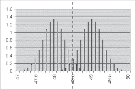
Figure 7.11 Upper limit for 
Figure 7.11 shows the distribution around 48 inches and the distribution around 49 inches for a sample large enough for the upper 95 percent (one-tail) limit for 48 inches to be 48.5 inches. In other words, this represents 5 percent of the distribution of mean values that fall above 48.5 inches if those samples are from a population with a true mean of 48 inches. Similarly, 5 percent of the mean values from samples in which the true mean of the population is 49 inches will fall below 48.5 inches. In this case, ![]() . Still assuming a standard deviation of height in the population of six-year-old boys as 10 inches, the nurse would have to select and measure a sample of about 1,150 six-year-old boys. A sample of 1,150! That seems very large.
. Still assuming a standard deviation of height in the population of six-year-old boys as 10 inches, the nurse would have to select and measure a sample of about 1,150 six-year-old boys. A sample of 1,150! That seems very large.
It is certainly feasible for the public health nurse to measure 1,150 six-year-old boys. But it is a much bigger job than measuring 100 six-year-old boys. Moreover, the county health officer may not be willing to grant her the time and resources away from her other duties to carry out a survey this large. Suppose instead that the county health officer agrees with the nurse that it may be useful to assess the effectiveness of the supplemental nutrition program for kindergarteners. They agree that the nurse can have the time and resources to select and measure a sample of 500 six-year-old boys. What then can be said of her perception that the program might have increased the height of six-year-old boys by one inch on the average?
If the nurse follows the prevailing tenets of statistical testing, which is to try to ensure against making the Type I error (rejecting the null hypothesis when it is true), she will set the upper 95 percent limit at about 48.75 inches. This result will be as seen in Figure 7.12, which shows the dashed vertical line at about 48.75 inches, so that 5 percent of the region of rejection of H0 will be above that value. But because the nurse has a sample of only 500, about 40 percent of the distribution around the mean of 49 percent is to the left of the dashed line. So while the nurse has only a 5 percent chance of rejecting H0 when it is true (Type I error), she has about a 40 percent chance of accepting H0 when it is false, and, in fact, H1 is true (a Type II error).

Figure 7.12 Positioning 
Avoiding Type I and Type II Errors
Both science and conventional logic are on the side of allowing a 40 percent Type II error, in the event that the nurse can select only a sample of 500 six-year-old boys. It is generally deemed less unattractive to say nothing happened than to say that something happened when we are not absolutely sure that it did (unless we are absolutely sure that something did happen). Thus, both science and conventional logic place the greatest emphasis on avoiding the Type I error.
But let us leave the realm of science for a moment and enter the realm of evaluation. The supplemental nutrition program has been in place for several years and has, in fact, become a fixture in the county. County supervisors have allocated funds for the program (to supplement grant funds received from the federal government) for the next 10 years. In essence, the supplemental nutrition program is already paid for. Only if it were shown that the program did not make any difference would the county supervisors be inclined to take the politically unattractive steps necessary to discontinue it. The program essentially costs less money at this stage than no program.
Under these circumstances, the public health nurse would be most concerned about not making the Type II error, the error of accepting H0 when it is false, or in terms of the program, the error of assuming that it had no effect when it actually did. If this were the case, the nurse—given that she is constrained to a sample of 500—might consciously set ![]() large enough so that the probability of the Type II error—
large enough so that the probability of the Type II error—![]() —would be low, say 0.05. She might do this even if it means that
—would be low, say 0.05. She might do this even if it means that ![]() must be larger than 0.05. If the nurse set
must be larger than 0.05. If the nurse set ![]() for
for ![]() and
and ![]() to 0.05, the result would be as that shown in Figure 7.13, wherein the area of acceptance of H0 has now been moved down to about 48.25 inches. Any sample value larger than that will be assumed to have come from a population in which the true mean value is 49 inches. In turn, the supplemental nutrition program will be deemed to have had an effect by its having increased the height of six-year-old boys. In this case, it is
to 0.05, the result would be as that shown in Figure 7.13, wherein the area of acceptance of H0 has now been moved down to about 48.25 inches. Any sample value larger than that will be assumed to have come from a population in which the true mean value is 49 inches. In turn, the supplemental nutrition program will be deemed to have had an effect by its having increased the height of six-year-old boys. In this case, it is ![]() that is large, being about 0.4, whereas
that is large, being about 0.4, whereas ![]() is about 0.05.
is about 0.05.

Figure 7.13 Low beta value
Although the logic discussed here might be reasonable, it is, in fact, rarely the case that a researcher would be willing to accept a value of ![]() as high as 0.4. Occasionally,
as high as 0.4. Occasionally, ![]() might be set as high as 0.1, or even 0.15. But higher levels of
might be set as high as 0.1, or even 0.15. But higher levels of ![]() , even to reduce
, even to reduce ![]() in situations such as those previously described, would be very unlikely.
in situations such as those previously described, would be very unlikely.
7.5 Selecting Sample Sizes
In dealing with confidence limits and Type I and Type II errors, the issue of sample size has come up several times. In particular, it was noted that in order for the public health nurse to be able to distinguish between ![]() and
and ![]() , she would have to have a sample of 1,150 six-year-old boys. How was that number derived?
, she would have to have a sample of 1,150 six-year-old boys. How was that number derived?
Sample Size and Confidence Level
If you recall the formula in Equation 7.1, 95 percent confidence limits are set by multiplying the t value for 95 percent (approximately 2) by the standard error of the mean. This value is then added to or subtracted from the mean to get the upper or lower limits of the confidence interval. What can be effectively varied in this formulation is the size of the standard error. As the sample size increases, the standard error will decrease, because it is the standard deviation divided by the square root of the sample size. Let us see what this means in regard to the confidence limits for a sample of six-year-old boys.
Measurement Error and Sample Size
We have said that the standard deviation of the height of six-year-old boys is 10 inches. Given that standard deviation, we can calculate the standard error for any given sample size. Knowing the standard error, we can calculate the size of the interval on either side of the sample mean value that will include the true population mean in 95 percent of all the samples. Statistically speaking, half of the confidence interval will be called the measurement error, and it will be designated ![]() .
. ![]() is defined as shown in Equation 7.3. As you can see, Equation 7.3 is just Equation 7.1 with the mean removed. It represents half of the total 95 percent confidence interval. In no case should
is defined as shown in Equation 7.3. As you can see, Equation 7.3 is just Equation 7.1 with the mean removed. It represents half of the total 95 percent confidence interval. In no case should ![]() be confused with the standard error.
be confused with the standard error.
Figure 7.14 shows the effect of sample size on the standard error, the measurement error ![]() , and the upper 95 percent limit for a mean of 48 inches, assuming a two-tail test (i.e., t in either Equation 7.1 or Equation 7.3 is 2; if a one-tail test were assumed, t would have to be approximately 1.7). For a sample of size 100, the standard error is 1 and
, and the upper 95 percent limit for a mean of 48 inches, assuming a two-tail test (i.e., t in either Equation 7.1 or Equation 7.3 is 2; if a one-tail test were assumed, t would have to be approximately 1.7). For a sample of size 100, the standard error is 1 and ![]() is 2. For a sample of 500, the standard error is 0.447 and
is 2. For a sample of 500, the standard error is 0.447 and ![]() is 0.894. For 1,150, the standard error is 0.295 and
is 0.894. For 1,150, the standard error is 0.295 and ![]() is 0.590. Although it is not immediately obvious from Figure 7.14, the size of both the standard error and
is 0.590. Although it is not immediately obvious from Figure 7.14, the size of both the standard error and ![]() decreases as the square root of the increase in sample size. For example, 1,150 is 11.5 times larger than 100. The standard error for a sample of 1,150, 0.295, is 3.39 times smaller than the standard error for a sample of 100. The square root of 11.5 is 3.39. This is a general result. The size of the standard error, and hence the size of
decreases as the square root of the increase in sample size. For example, 1,150 is 11.5 times larger than 100. The standard error for a sample of 1,150, 0.295, is 3.39 times smaller than the standard error for a sample of 100. The square root of 11.5 is 3.39. This is a general result. The size of the standard error, and hence the size of ![]() , decreases as the square root of the increase in sample size. So if sample size doubles,
, decreases as the square root of the increase in sample size. So if sample size doubles, ![]() decreases by 1.44. If sample size increases by a factor of 9,
decreases by 1.44. If sample size increases by a factor of 9, ![]() decreases by a factor of 3.
decreases by a factor of 3.

Figure 7.14 Effect of sample size on standard error and measurement error
How to Determine Sample Size
If you know the standard deviation, you can set the standard error, and thus the confidence interval, virtually anywhere you like. You just need to have the resources required to obtain the sample size needed. The actual formula for determining the sample size, given knowledge of the standard deviation and a good idea of how large ![]() should be, is given in Equation 7.4. This equation says that the sample size n is equal to the square of the value of t times the square of the standard deviation divided by the square of whatever the error of measurement,
should be, is given in Equation 7.4. This equation says that the sample size n is equal to the square of the value of t times the square of the standard deviation divided by the square of whatever the error of measurement, ![]() , is expected to be.
, is expected to be.
Equation 7.4 would seem to have an intellectually soothing quality. If you know how much measurement error you can tolerate, then you can set the sample size necessary for that error. For example, in the case of the public health nurse who wished to distinguish between an average height of 49 inches and an average height of 48 inches, measurement error required 0.5 inches. Apart from the problem that the sample size set may be quite large and therefore quite expensive, there is another problem. This is the problem of knowledge of the variance ![]() in Equation 7.4. In general, it is necessary to collect some data and calculate the variance before the variance is known. So, in order to determine how large a sample is required, it is already necessary to have some sample data. This is in the nature of a statistical catch-22.
in Equation 7.4. In general, it is necessary to collect some data and calculate the variance before the variance is known. So, in order to determine how large a sample is required, it is already necessary to have some sample data. This is in the nature of a statistical catch-22.
There is one realm, however, in which the standard deviation can be known before any data are collected. The variance of a proportion can be calculated directly from the proportion as the square root of the proportion times 1 minus the proportion. So, for example, if you have some general knowledge of the size of a proportion to be estimated, it is possible to determine the sample size necessary to be within some specified measurement error by Equation 7.5.