
CHAPTER 7
Large Sample Theory for Estimation and Testing
PART I: THEORY
We have seen in the previous chapters several examples in which the exact sampling distribution of an estimator or of a test statistic is difficult to obtain analytically. Large samples yield approximations, called asymptotic approximations, which are easy to derive, and whose error decreases to zero as the sample size grows. In this chapter, we discuss asymptotic properties of estimators and of test statistics, such as consistency, asymptotic normality, and asymptotic efficiency. In Chapter 1, we presented results from probability theory, which are necessary for the development of the theory of asymptotic inference. Section 7.1 is devoted to the concept of consistency of estimators and test statistics. Section 7.2 presents conditions for the strong consistency of the maximum likelihood estimator (MLE). Section 7.3 is devoted to the asymptotic normality of MLEs and discusses the notion of best asymptotically normal (BAN) estimators. In Section 7.4, we discuss second and higher order efficiency. In Section 7.5, we present asymptotic confidence intervals. Section 7.6 is devoted to Edgeworth and saddlepoint approximations to the distribution of the MLE, in the one–parameter exponential case. Section 7.7 is devoted to the theory of asymptotically efficient test statistics. Section 7.8 discusses the Pitman’s asymptotic efficiency of tests.
7.1 CONSISTENCY OF ESTIMATORS AND TESTS
Consistency of an estimator is a property, which guarantees that in large samples, the estimator yields values close to the true value of the parameter, with probability close to one. More formally, we define consistency as follows.
Definition 7.1.1 Let {![]() n;n = n0, n0 + 1, … } be a sequence of estimators of a parameter θ.
n;n = n0, n0 + 1, … } be a sequence of estimators of a parameter θ. ![]() n is called consistent if
n is called consistent if ![]() n
n ![]() θ as n → ∞. The sequence is called strongly consistent if θn → θ almost surely (a.s.) as n→ ∞ for all θ.
θ as n → ∞. The sequence is called strongly consistent if θn → θ almost surely (a.s.) as n→ ∞ for all θ.
Different estimators of a parameter θ might be consistent. Among the consistent estimators, we would prefer those having asymptotically, smallest mean squared error (MSE). This is illustrated in Example 7.2.
As we shall see later, the MLE is asymptotically most efficient estimator under general regularity conditions.
We conclude this section by defining the consistency property for test functions.
Definition 7.1.2. Let {![]() n} be a sequence of test functions, for testing H0: θ
n} be a sequence of test functions, for testing H0: θ ![]() Θ0 versus H1: θ
Θ0 versus H1: θ ![]() Θ1. The sequence {
Θ1. The sequence {![]() n} is called consistent if
n} is called consistent if
A test function ![]() n satisfying property (i) is called asymptotically size α test.
n satisfying property (i) is called asymptotically size α test.
All test functions discussed in Chapter 4 are consistent. We illustrate in Example 7.3 a test which is not based on an explicit parametric model of the distribution F(x). Such a test is called a distribution free test, or a nonparametric test. We show that the test is consistent.
As in the case of estimation, it is not sufficient to have consistent test functions. One should consider asymptotically efficient tests, in a sense that will be defined later.
7.2 CONSISTENCY OF THE MLE
The question we address here is whether the MLE is consistent. We have seen in Example 5.22 a case where the MLE is not consistent; thus, one needs conditions for consistency of the MLE. Often we can prove the consistency of the MLE immediately, as in the case of the MLE of θ = (μ, σ) in the normal case, or in the Binomial and Poisson distributions.
Let X1, X2, …,Xn, … be independent identically distributed (i.i.d.) random variables having a p.d.f. f(x; θ), θ ![]() Θ. Let
Θ. Let
![]()
If θ0 is the parameter value of the distribution of the Xs, then from the strong law of large numbers (SLLN)
as n→ ∞, where I(θ0, θ) is the Kullback–Leibler information. Assume that I(θ0, θ′) > 0 for all θ′ ≠ θ0. Since the MLE, ![]() n, maximizes the left–hand side of (7.2.1) and since I(θ0, θ0) = 0, we can immediately conclude that if Θ contains only a finite number of points, then the MLE is strongly consistent. This result is generalized in the following theorem.
n, maximizes the left–hand side of (7.2.1) and since I(θ0, θ0) = 0, we can immediately conclude that if Θ contains only a finite number of points, then the MLE is strongly consistent. This result is generalized in the following theorem.
Theorem 7.2.1. Let X1, …,Xn be i.i.d. random variables having a p.d.f. f(x;θ), θ ![]() Θ, and let θ0 be the true value of θ. If
Θ, and let θ0 be the true value of θ. If
then the MLE ![]() n
n ![]() θ0, as n→ ∞.
θ0, as n→ ∞.
The proof is outlined only. For δ > 0, let Θδ = {θ: |θ − θ0|≥ δ }. Since Θ is compact so is Θδ. Let U(X; θ) = log f(X; θ) − log f(X; θ0). The conditions of the theorem imply (see Ferguson, 1996, p. 109) that
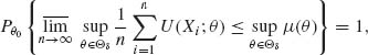
where μ (θ) = −I(θ0, θ) < 0, for all θ ![]() Θδ. Thus, with probability one, for n sufficiently large,
Θδ. Thus, with probability one, for n sufficiently large,
![]()
But,
![]()
Thus, with probability one, for n sufficiently large, |![]() n − θ0| < δ. This demonstrates the consistency of the MLE.
n − θ0| < δ. This demonstrates the consistency of the MLE.
For consistency theorems that require weaker conditions, see Pitman (1979, Ch. 8). For additional reading, see Huber (1967), Le Cam (1986), and Schervish (1995, p. 415).
7.3 ASYMPTOTIC NORMALITY AND EFFICIENCY OF CONSISTENT ESTIMATORS
The presentation of concepts and theory is done in terms of real parameter θ. The results are generalized to k–parameters cases in a straightforward manner.
A consistent estimator ![]() (Xn) of θ is called asymptotically normal if, there exists an increasing sequence {cn}, cn
(Xn) of θ is called asymptotically normal if, there exists an increasing sequence {cn}, cn ![]() ∞ as n→ ∞, so that
∞ as n→ ∞, so that
(7.3.1) ![]()
The function AV{![]() n} = v2(θ) /
n} = v2(θ) /![]() is called the asymptotic variance of
is called the asymptotic variance of ![]() (Xn). Let S(Xn;θ) =
(Xn). Let S(Xn;θ) = ![]() log f(Xi; θ) be the score function and I(θ) the Fisher information. An estimator
log f(Xi; θ) be the score function and I(θ) the Fisher information. An estimator ![]() n that, under the Cramér–Rao (CR) regularity conditions, satisfies
n that, under the Cramér–Rao (CR) regularity conditions, satisfies
as n→ ∞, is called asymptotically efficient. Recall that, by the Central Limit Theorem (CLT), ![]() S (Xn;θ)
S (Xn;θ) ![]() N(0,I(θ)). Thus, efficient estimators satisfying (7.3.2) have the asymptotic property that
N(0,I(θ)). Thus, efficient estimators satisfying (7.3.2) have the asymptotic property that
For this reason, such asymptotically efficient estimators are also called BAN estimators.
We show now a set of conditions under which the MLE ![]() n is a BAN estimator.
n is a BAN estimator.
In Example 1.24, we considered a sequence {Xn} of i.i.d. random variables, with X1 ∼ B(1,θ), 0 < θ < 1. In this case, ![]() n =
n = ![]()
![]() Xi is a strongly consistent estimator of θ. The variance stabilizing transformation g(
Xi is a strongly consistent estimator of θ. The variance stabilizing transformation g(![]() n) = 2 sin −1
n) = 2 sin −1![]() is a (strongly) consistent estimator of ω = 2 sin −1
is a (strongly) consistent estimator of ω = 2 sin −1![]() . This estimator is asymptotically normal with an asymptotic variance AV{g(
. This estimator is asymptotically normal with an asymptotic variance AV{g(![]() n)} =
n)} = ![]() for all ω.
for all ω.
Although consistent estimators satisfying (7.3.3) are called BAN, one can construct sometimes asymptotically normal consistent estimators, which at some θ values have an asymptotic variance, with v2(θ) < ![]() . Such estimators are called super efficient. In Example 7.5, we illustrate such an estimator.
. Such estimators are called super efficient. In Example 7.5, we illustrate such an estimator.
Le Cam (1953) proved that the set of point on which ![]() has a Lebesgue measure zero, as in Example 7.5.
has a Lebesgue measure zero, as in Example 7.5.
The following are sufficient conditions for a consistent MLE to be a BAN estimator.
Theorem 7.3.1 (Asymptotic efficiency of MLE). Let ![]() n be an MLE of θ then, under conditions C.1.–C.4.
n be an MLE of θ then, under conditions C.1.–C.4.
![]()
Sketch of the Proof. Let Bδ, θ, n be a Borel set in ![]() n such that, for all Xn
n such that, for all Xn ![]() Bδ, θ, n,
Bδ, θ, n, ![]() n exists and S(Xn;
n exists and S(Xn; ![]() n) = 0. Moreover, Pθ (Bδ, θ, n) ≥ 1 − δ. For Xn
n) = 0. Moreover, Pθ (Bδ, θ, n) ≥ 1 − δ. For Xn ![]() Bδ, θ, n, consider the expansion
Bδ, θ, n, consider the expansion
![]()
where |![]() − θ| ≤ |
− θ| ≤ |![]() n − θ|.
n − θ|.
According to conditions (iii)–(v) in Theorem 7.2.1, and Slutzky’s Theorem,
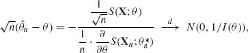
as n→ ∞, since by the CLT
![]()
as n→ ∞.
7.4 SECOND–ORDER EFFICIENCY OF BAN ESTIMATORS
Often BAN estimators ![]() n are biased, with
n are biased, with
(7.4.1) ![]()
The problem then is how to compare two different BAN estimators of the same parameter. Due to the bias, the asymptotic variance may not present their precision correctly, when the sample size is not extremely large. Rao (1963) suggested to adjust first an estimator ![]() n to reduce its bias to an order of magnitude of 1/n2. Let
n to reduce its bias to an order of magnitude of 1/n2. Let ![]() be the adjusted estimator, and let
be the adjusted estimator, and let
(7.4.2) ![]()
The coefficient D of 1/n2 is called the second–order deficiency coefficient. Among two BAN estimators, we prefer the one having a smaller second–order deficiency coefficient.
Efron (1975) analyzed the structure of the second–order coefficient D in exponential families in terms of their curvature, the Bhattacharyya second–order lower bound, and the bias of the estimators. Akahira and Takeuchi (1981) and Pfanzagl (1985) established the structure of the distributions of asymptotically high orders most efficient estimators. They have shown that under the CR regularity conditions, the distribution of the most efficient second–order estimator ![]() is
is
(7.4.3) ![]()
where
(7.4.4) ![]()
and
(7.4.5) ![]()
For additional reading, see also Barndorff–Nielsen and Cox (1994).
7.5 LARGE SAMPLE CONFIDENCE INTERVALS
Generally, the large sample approximations to confidence limits are based on the MLEs of the parameter(s) under consideration. This approach is meaningful in cases where the MLEs are known. Moreover, under the regularity conditions given in the theorem of Section 7.3, the MLEs are BAN estimators. Accordingly, if the sample size is large, one can in regular cases employ the BAN property of MLE to construct confidence intervals around the MLE. This is done by using the quantiles of the standard normal distribution, and the square root of the inverse of the Fisher information function as the standard deviation of the (asymptotic) sampling distribution. In many situations, the inverse of the Fisher information function depends on the unknown parameters. The practice is to substitute for the unknown parameters their respective MLEs. If the samples are very large this approach may be satisfactory. However, as will be shown later, if the samples are not very large it may be useful to apply first a variance stabilizing transformationg(θ) and derive the confidence limits of g(θ).
A transformation g(θ) is called variance stabilizing if g′(θ) = ![]() . If
. If ![]() n is an MLE of θ then g(
n is an MLE of θ then g(![]() n) is an MLE of g(θ). The asymptotic variance of g(
n) is an MLE of g(θ). The asymptotic variance of g(![]() n) under the regularity conditions is (g′(θ))2/nI(θ). Accordingly, if g′(θ) =
n) under the regularity conditions is (g′(θ))2/nI(θ). Accordingly, if g′(θ) = ![]() then the asymptotic variance of g(
then the asymptotic variance of g(![]() n) is
n) is ![]() . For example, suppose that X1, …,Xn is a sample of n i.i.d. binomial random variables, B(1,θ). Then, the MLE of θ is
. For example, suppose that X1, …,Xn is a sample of n i.i.d. binomial random variables, B(1,θ). Then, the MLE of θ is ![]() n. The Fisher information function is In(θ) = n/θ (1 − θ). If g(θ) = 2 sin−1
n. The Fisher information function is In(θ) = n/θ (1 − θ). If g(θ) = 2 sin−1![]() then g′(θ) = 1/
then g′(θ) = 1/![]() . Hence, the asymptotic variance of g(
. Hence, the asymptotic variance of g(![]() n) = 2 sin−1
n) = 2 sin−1 ![]() is
is ![]() . Transformations stabilizing whole covariance matrices are discussed in the paper of Holland (1973).
. Transformations stabilizing whole covariance matrices are discussed in the paper of Holland (1973).
Let θ = t(g) be the inverse of a variance stabilizing transformation g(θ), and suppose (without loss of generality) that t(g) is strictly increasing. For cases satisfying the BAN regularity conditions, if ![]() n is the MLE of θ,
n is the MLE of θ,
(7.5.1) ![]()
A (1 − α) confidence interval for g(θ) is given asymptotically by (g(![]() n) − z1 − α /2/
n) − z1 − α /2/![]() , g(
, g(![]() n) + z1 − α /2/
n) + z1 − α /2/![]() ), where z1 − α /2 = Φ −1(1 − α /2). Let gL and gU denote these lower and upper confidence intervals. We assume that both limits are within the range of the function g(θ); otherwise, we can always truncate it in an appropriate manner. After obtaining the limits gL and gU we make the inverse transformation on these limits and thus obtain the limits θL = t(gL) and θU = t(gU). Indeed, since t(g) is a one–to–one increasing transformation,
), where z1 − α /2 = Φ −1(1 − α /2). Let gL and gU denote these lower and upper confidence intervals. We assume that both limits are within the range of the function g(θ); otherwise, we can always truncate it in an appropriate manner. After obtaining the limits gL and gU we make the inverse transformation on these limits and thus obtain the limits θL = t(gL) and θU = t(gU). Indeed, since t(g) is a one–to–one increasing transformation,
(7.5.2) 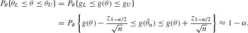
Thus, (θL, θU) is an asymptotically (1−α)–confidence interval.
7.6 EDGEWORTH AND SADDLEPOINT APPROXIMATIONS TO THE DISTRIBUTION OF THE MLE: ONE–PARAMETER CANONICAL EXPONENTIAL FAMILIES
The asymptotically normal distributions for the MLE require often large samples to be effective. If the samples are not very large one could try to modify or correct the approximation by the Edgeworth expansion. We restrict attention in this section to the one–parameter exponential type families in canonical form.
According to (5.6.2), the MLE, ![]() n, of the canonical parameter
n, of the canonical parameter ![]() satisfies the equation
satisfies the equation
(7.6.1) ![]()
The cumulant generating function K(![]() ) is analytic. Let G(x) be the inverse function of K′(
) is analytic. Let G(x) be the inverse function of K′(![]() ). G(x) is also analytic and one can write, for large samples,
). G(x) is also analytic and one can write, for large samples,
(7.6.2) 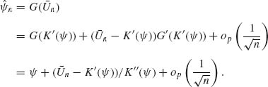
Recall that K″(![]() ) = I(
) = I(![]() ) is the Fisher information function, and for large samples,
) is the Fisher information function, and for large samples,
(7.6.3) ![]()
Moreover, E{![]() n} = K′(
n} = K′(![]() ) and V{
) and V{![]()
![]() n} = I(
n} = I(![]() ). Thus, by the CLT,
). Thus, by the CLT,
(7.6.4) ![]()
Equivalently,
(7.6.5) ![]()
This is a version of Theorem 7.3.1, in the present special case.
If the sample is not very large, we can add terms to the distribution of ![]() according to the Edgeworth expansion. We obtain
according to the Edgeworth expansion. We obtain
(7.6.6) 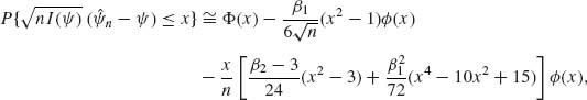
where
(7.6.7) ![]()
and
(7.6.8) ![]()
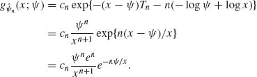
Let Tn = ![]() U(Xi). Tn is the likelihood statistic. As shown in Reid (1988) the saddlepoint approximation to the p.d.f. of the MLE,
U(Xi). Tn is the likelihood statistic. As shown in Reid (1988) the saddlepoint approximation to the p.d.f. of the MLE, ![]() n, is
n, is
where cn is a factor of proportionality, such that ![]() g
g![]() n (x;
n (x; ![]() )dμ (x) = 1.
)dμ (x) = 1.
Let L(θ; Xn) and l(θ ;Xn) denote the likelihood and log–likelihood functions. Let ![]() n denotes the MLE of θ, and
n denotes the MLE of θ, and
(7.6.10) ![]()
We have seen that Eθ {Jn(θ)} = I(θ). Thus, Jn(θ) ![]() I(θ), as n→ ∞ (the Fisher information function). Jn(
I(θ), as n→ ∞ (the Fisher information function). Jn(![]() n) is an MLE estimator of Jn(θ). Thus, if
n) is an MLE estimator of Jn(θ). Thus, if ![]() n
n ![]() θ, as n→ ∞, then, as in condition C.4. of Theorem 7.3.1, Jn(
θ, as n→ ∞, then, as in condition C.4. of Theorem 7.3.1, Jn(![]() n)
n) ![]() I(θ), as n→ ∞. The saddlepoint approximation to g
I(θ), as n→ ∞. The saddlepoint approximation to g![]() n (x;θ) in the general regular case is
n (x;θ) in the general regular case is
Formula (7.6.11) is called the Barndorff–Nielsen p*–formula. The order of magnitude of its error, in large samples, is O(n−3/2).
7.7 LARGE SAMPLE TESTS
For testing two simple hypotheses there exists a most powerful test of size α. We have seen examples in which it is difficult to determine the exact critical level kα of the test. Such a case was demonstrated in Example 4.4. In that example, we have used the asymptotic distribution of the test statistic to approximate kα. Generally, if X1, …,Xn are i.i.d. with common p.d.f. f(x;θ) let
(7.7.1) ![]()
where the two sample hypotheses are H0: θ = θ0 and H1: θ = θ1. The most powerful test of size α can be written as
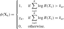
Thus, in large samples we can consider the test function ![]() (Sn) = I{Sn ≥ kα }, where Sn =
(Sn) = I{Sn ≥ kα }, where Sn = ![]() log R(Xi). Note that under H0, Eθ0{Sn} = −n(I(θ0, θ1) while under H1, Eθ1{Sn} = nI(θ1, θ0), where I(θ, θ′) is the Kullback–Leibler information.
log R(Xi). Note that under H0, Eθ0{Sn} = −n(I(θ0, θ1) while under H1, Eθ1{Sn} = nI(θ1, θ0), where I(θ, θ′) is the Kullback–Leibler information.
Let ![]() = Vθ0{log R(X1)}. Assume that 0 <
= Vθ0{log R(X1)}. Assume that 0 < ![]() < ∞. Then, by the CLT,
< ∞. Then, by the CLT, ![]() = Φ (x). Hence, a large sample approximation to kα is
= Φ (x). Hence, a large sample approximation to kα is
(7.7.2) ![]()
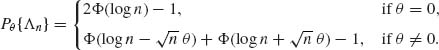
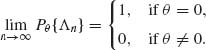
The large sample approximation to the power of the test is
(7.7.3) ![]()
where σ![]() = Vθ1{log R(X1)}. Generally, for testing H0: θ = θ0 versus H1: θ ≠ θ0 where θ is a k–parameter vector, the following three test statistics are in common use, in cases satisfying the CR regularity condition:
= Vθ1{log R(X1)}. Generally, for testing H0: θ = θ0 versus H1: θ ≠ θ0 where θ is a k–parameter vector, the following three test statistics are in common use, in cases satisfying the CR regularity condition:
(7.7.4) ![]()
where ![]() n is the MLE of θ, and
n is the MLE of θ, and
(7.7.5) ![]()
Here, H(θ) is the matrix of partial derivatives
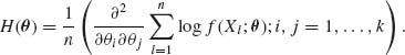
An alternative statistic, which is asymptotically equivalent to Qw, is
(7.7.6) ![]()
One could also use the FIM, I(θ0), instead of J(θ0).
(7.7.7) ![]()
(7.7.8) ![]()
where S(Xn;θ) is the score function, namely, the gradient vector ![]() θ
θ ![]() log f(Xi; θ). QR does not require the computation of the MLE
log f(Xi; θ). QR does not require the computation of the MLE ![]() n.
n.
On the basis of the multivariate asymptotic normality of ![]() n, we can show that all these three test statistics have in the regular cases, under H0, an asymptotic χ2[k] distribution. The asymptotic power function can be computed on the basis of the non–central χ2[k;λ] distribution.
n, we can show that all these three test statistics have in the regular cases, under H0, an asymptotic χ2[k] distribution. The asymptotic power function can be computed on the basis of the non–central χ2[k;λ] distribution.
7.8 PITMAN’S ASYMPTOTIC EFFICIENCY OF TESTS
The Pitman’s asymptotic efficiency is an index of the relative performance of test statistics in large samples. This index is called the Pitman’s asymptotic relative efficiency (ARE). It was introduced by Pitman in 1948.
Let X1, …,Xn be i.i.d. random variables, having a common distribution F(x;θ), θ ![]() Θ. Let Tn be a statistic. Suppose that there exist functions μ (θ) and σn(θ) so that, for each θ
Θ. Let Tn be a statistic. Suppose that there exist functions μ (θ) and σn(θ) so that, for each θ ![]() Θ, Zn = (Tn − μ (θ))/σn(θ)
Θ, Zn = (Tn − μ (θ))/σn(θ)![]() N(0,1), as n→ ∞. Often σn(θ) = c(θ) w(n), where w(n) = n−α for some α > 0.
N(0,1), as n→ ∞. Often σn(θ) = c(θ) w(n), where w(n) = n−α for some α > 0.
Consider the problem of testing the hypotheses H0: θ ≤ θ0 against H1: θ > θ0, at level αn → α, as n→ ∞. Let the sequence of test functions be
(7.8.1) ![]()
where kn → Z1 − α. The corresponding power functions are
(7.8.2) ![]()
We assume that
Under these assumptions, if θn = θ0 + δ w(n) then, with δ > 0,
(7.8.3) ![]()
The function
(7.8.4) ![]()
is called the asymptotic efficacy of Tn.
Let Vn be an alternative test statistic, and Wn = (Vn − η (θ))/(v(θ)w(n))![]() N(0,1), as n→ ∞. The asymptotic efficacy of Vn is J(θ;V) = (η′(θ))2/v2(θ). Consider the case of w(n) = n−1/2. Let θn = θ0 +
N(0,1), as n→ ∞. The asymptotic efficacy of Vn is J(θ;V) = (η′(θ))2/v2(θ). Consider the case of w(n) = n−1/2. Let θn = θ0 + ![]() , δ > 0, be a sequence of local alternatives. Let
, δ > 0, be a sequence of local alternatives. Let ![]() n(θn;Vn) be the sequence of power functions at θn = θ0 + δ /
n(θn;Vn) be the sequence of power functions at θn = θ0 + δ /![]() and sample size n′(n) so that
and sample size n′(n) so that ![]()
![]() n′(θn; Vn′) =
n′(θn; Vn′) = ![]() =
= ![]()
![]() n(θn; Tn). For this
n(θn; Tn). For this
(7.8.5) ![]()
and
This limit (7.8.6) is the Pitman ARE of Vn relative to Tn.
We remark that the asymptotic distributions of Zn and Wn do not have to be N(0,1), but they should be the same. If Zn and Wn converge to two different distributions, the Pitman ARE is not defined.
7.9 ASYMPTOTIC PROPERTIES OF SAMPLE QUANTILES
Give a random sample of n i.i.d. random variables, the empirical distribution of the sample is
(7.9.1) ![]()
This is a step function, with jumps of size 1/n at the location of the sample random variables {Xi, i = 1, …,n}. The pth quantile of a distribution F is defined as
(7.9.2) ![]()
according to this definition the quanitles are unique. Similarly, the pth sample quantile are defined as ξn,p = ![]() (p).
(p).
Theorem 7.9.1. Let 0 < p < 1. Suppose that F is differentiable at the pth quantile ξp, and F′(ξp) > 0, then ξn,p → ξp a.s. as n→ ∞.
Proof. Let ![]() > 0 then
> 0 then
![]()
By SLLN
![]()
and
![]()
Hence,
![]()
as n→ ∞. Thus,
![]()
as n→ ∞. That is,
![]() QED
QED
Note that if 0 < F(ξ) < 1 then, by CLT,
(7.9.3) ![]()
for all −∞ < t < ∞. We show now that, under certain conditions, ξn,p is asymptotically normal.
Theorem 7.9.2. Let 0 < p < 1. Suppose that F is continuous at ξp = F−1(p). Then,
(7.9.4) ![]()
(7.9.5) 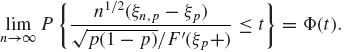
Proof. Fix t. Let A > 0 and define
(7.9.6) ![]()
Thus,
(7.9.7) 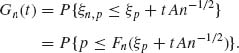
Moreover, since nFn(ξp) ∼ B(n, F(ξp)),
(7.9.8) ![]()
By CLT,
(7.9.9) ![]()
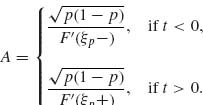
as n→ ∞, where ![]() (ξp) = 1 − F(ξp). Let
(ξp) = 1 − F(ξp). Let
(7.9.10) ![]()
and
(7.9.11) ![]()
Then
where
(7.9.13) ![]()
Since F is continuous at ξp,
![]()
Moreover, if ![]() . Hence, if t > 0
. Hence, if t > 0
(7.9.14) ![]()
Similarly, if t < 0
(7.9.15) ![]()
Thus, let
Then, ![]() Cn(t) = t. Hence, from (7.9.12),
Cn(t) = t. Hence, from (7.9.12),
![]() QED
QED
Corollary. If F is differentiable at ξp, and f(ξp) = ![]() F(x) |x=ξp> 0, then ξn,p is asymptotically N
F(x) |x=ξp> 0, then ξn,p is asymptotically N ![]() .
.
PART II: EXAMPLES
Example 7.1. Let X1, X2, … be a sequence of i.i.d. random variables, such that E{|X1|} < ∞. By the SLLN, ![]() n =
n = ![]()
![]() Xi
Xi ![]() μ, as n→ ∞, where μ = E{X1}. Thus, the sample mean
μ, as n→ ∞, where μ = E{X1}. Thus, the sample mean ![]() n is a strongly consistent estimator of μ. Similarly, if E{|X1|r} < ∞, r≥ 1, then the rth sample moment Mn,r is strongly consistent estimator of μr = E{
n is a strongly consistent estimator of μ. Similarly, if E{|X1|r} < ∞, r≥ 1, then the rth sample moment Mn,r is strongly consistent estimator of μr = E{![]() }, i.e.,
}, i.e.,
![]()
Thus, if σ2 = V{X1}, and 0 < σ2 < ∞,
![]()
That is, ![]() is a strongly consistent estimator of σ2. It follows that
is a strongly consistent estimator of σ2. It follows that ![]() =
= ![]()
![]() (Xi −
(Xi − ![]() n)2 is also a strongly consistent estimator of σ2. Note that, since Mn,r
n)2 is also a strongly consistent estimator of σ2. Note that, since Mn,r ![]() μr, as n→ ∞ whenever E{|X1|r} < ∞, then for any continuous function g(·), g(Mn,r)
μr, as n→ ∞ whenever E{|X1|r} < ∞, then for any continuous function g(·), g(Mn,r) ![]() g(μr), as n→ ∞. Thus, if
g(μr), as n→ ∞. Thus, if
![]()
is the coefficient of skewness, the sample coefficient of skewness is strongly consistent estimator of β1, i.e.,
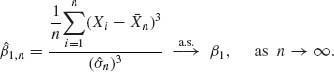
![]()
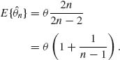
Example 7.2. Let X1, X2, … be a sequence of i.i.d. random variables having a rectangular distribution R(0, θ), 0 < θ < ∞. Since μ1 = θ /2, ![]() 1,n = 2
1,n = 2![]() n is a strongly consistent estimator of θ. The MLE
n is a strongly consistent estimator of θ. The MLE ![]() 2,n = X(n) is also strongly consistent estimator of θ. Actually, since for any 0 <
2,n = X(n) is also strongly consistent estimator of θ. Actually, since for any 0 < ![]() < θ,
< θ,
![]()
Hence, by Borel–Cantelli Lemma, P{![]() 2,n ≤ θ −
2,n ≤ θ − ![]() , i.o.} = 0. This implies that
, i.o.} = 0. This implies that ![]() 2,n
2,n ![]() θ, as n→ ∞. The MLE is strongly consistent. The expected value of the MLE is E{
θ, as n→ ∞. The MLE is strongly consistent. The expected value of the MLE is E{![]() 2,n} =
2,n} = ![]() θ. The variance of the MLE is
θ. The variance of the MLE is
![]()
The MSE of {![]() 2,n} is V{
2,n} is V{![]() 2,n} + Bias2{
2,n} + Bias2{![]() 2,n}, i.e.,
2,n}, i.e.,
![]()
The variance of ![]() 1,n is V{
1,n is V{![]() 1,n} =
1,n} = ![]() . The relative efficiency of
. The relative efficiency of ![]() 1,n against
1,n against ![]() 2,n is
2,n is
![]()
as n→ ∞. Thus, in large samples, 2![]() n is very inefficient estimator relative to the MLE.
n is very inefficient estimator relative to the MLE. ![]()
Example 7.3. Let X1, X2, …, Xn be i.i.d. random variables having a continuous distribution F(x), symmetric around a point θ. θ is obviously the median of the distribution, i.e., ![]() . We index these distributions by θ and consider the location family
. We index these distributions by θ and consider the location family ![]() s = {Fθ: Fθ (x) = F(x − θ), and F(−z) = 1−F(z); −∞ < θ < ∞ }. The functional form of F is not specified in this model. Thus,
s = {Fθ: Fθ (x) = F(x − θ), and F(−z) = 1−F(z); −∞ < θ < ∞ }. The functional form of F is not specified in this model. Thus, ![]() s is the family of all symmetric, continuous distributions. We wish to test the hypotheses
s is the family of all symmetric, continuous distributions. We wish to test the hypotheses
![]()
The following test is the Wilcoxon signed–rank test:
Let Yi = Xi − θ0, i = 1, …,n. Let S(Yi) = I{Yi > 0}, i = 1, …,n. We consider now the ordered absolute values of Yi, i.e.,
![]()
and let R(Yi) be the index (j) denoting the place of Yi in the ordered absolute values, i.e., R(Yi) = j, j = 1, …,n if, and only if, |Yi| = |Y|(j). Define the test statistic
![]()
The test of H0 versus H1 based on Tn, which rejects H0 if Tn is sufficiently large is called the Wilcoxon signed–rank test. We show that this test is consistent. Note that under H0, P0{S(Yi) = 1} = ![]() . Moreover, for each i = 1, …, n, under H0
. Moreover, for each i = 1, …, n, under H0
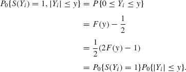
Thus, S(Yi) and |Yi| are independent. This implies that, under H0, S(Y1), …, S(Yn) are independent of R(Y1), …,R(Yn), and the distribution of Tn, under H0, is like that of Tn = ![]() jWj ∼
jWj ∼ ![]() jB
jB![]() . It follows that, under H0,
. It follows that, under H0,
Similarly, under H0,
According to Problem 3 of Section 1.12, the CLT holds, and
![]()
Thus, the test function
has, asymptotically size α, 0 < α < 1. This establishes part (i) of the definition of consistency.
When θ > θ0 (under H1) the distribution of Tn is more complicated. We can consider the test statistic Vn = ![]() One can show (see Hettmansperger, 1984, p. 47) that the asymptotic mean of Vn, as n→ ∞, is
One can show (see Hettmansperger, 1984, p. 47) that the asymptotic mean of Vn, as n→ ∞, is ![]() p2(θ), and the asymptotic variance of Vn is
p2(θ), and the asymptotic variance of Vn is
![]()
where
![]()
In addition, one can show that the asymptotic distribution of Vn (under H1) is normal (see Hettmansperger, 1984).
Finally, when θ > 0, p2(θ) > ![]() and
and
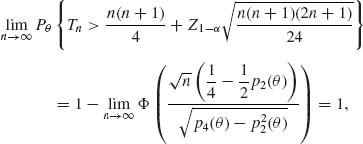
for all θ > 0. Thus, the Wilcoxon signed–rank test is consistent. ![]()
Example 7.4. Let T1, T2, …, Tn be i.i.d. random variables having an exponential distribution with mean β, 0 < β < ∞. The observable random variables are Xi = min (Ti, t*), i = 1, …,n; 0 < t* < ∞. This is the case of Type I censoring of the random variables T1, …, Tn.
The likelihood function of β, 0 < β < ∞, is
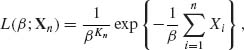
where Kn = ![]() I{Xi < t }. Note that the MLE of β does not exist if Kn = 0. However, P{Kn = 0} = e−nt* /β → 0 as n→ ∞. Thus, for sufficiently large n, the MLE of β is
I{Xi < t }. Note that the MLE of β does not exist if Kn = 0. However, P{Kn = 0} = e−nt* /β → 0 as n→ ∞. Thus, for sufficiently large n, the MLE of β is

Note that by the SLLN,
![]()
and
![]()
Moreover,
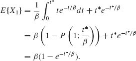
Thus, ![]() n
n ![]() β, as n→ ∞. This establishes the strong consistency of
β, as n→ ∞. This establishes the strong consistency of ![]() n.
n. ![]()
Example 7.5. Let {Xn} be a sequence of i.i.d. random variables, X1 ∼ N(θ, 1), −∞ < θ < ∞. Given a sample of n observations, the minimal sufficient statistic is ![]() n =
n = ![]()
![]() Xj. The Fisher information function is I(θ) = 1, and
Xj. The Fisher information function is I(θ) = 1, and ![]() n is a BAN estimator. Consider the estimator,
n is a BAN estimator. Consider the estimator,
Let
![]()
Now,
Thus,
We show now that ![]() n is consistent. Indeed, for any δ > 0,
n is consistent. Indeed, for any δ > 0,
![]()
If θ = 0 then
![]()
since ![]() n is consistent. Similarly, if θ ≠ 0,
n is consistent. Similarly, if θ ≠ 0,
![]()
Thus, ![]() n is consistent. Furthermore,
n is consistent. Furthermore,
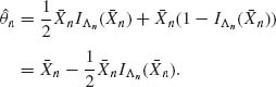
Hence,
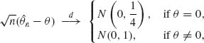
as n→ ∞. This shows that ![]() n is asymptotically normal, with asymptotic variance
n is asymptotically normal, with asymptotic variance
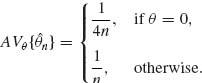
![]() n is super efficient.
n is super efficient. ![]()
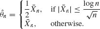
Example 7.6. Let X1, X2, …, Xn be i.i.d. random variables, X1 ∼ B(1,e−θ), 0 < θ < ∞. The MLE of θ after n observations is
![]() n does not exist if
n does not exist if ![]() Xi = 0. The probability of this event is (1−e−θ)n. Thus, if n ≥ N(δ, θ) =
Xi = 0. The probability of this event is (1−e−θ)n. Thus, if n ≥ N(δ, θ) = ![]() , then Pθ
, then Pθ  < δ. For n ≥ N(δ, θ), let
then Pθ {Bn} > 1 − δ. On the set Bn, ![]() , where
, where ![]() n =
n = ![]()
![]() Xi is the MLE of p = e−θ. Finally, the Fisher information function is I(θ) = e−θ/ (1 − e−θ), and
Xi is the MLE of p = e−θ. Finally, the Fisher information function is I(θ) = e−θ/ (1 − e−θ), and
![]()
All the conditions of Theorem 7.3.1 hold, and
![]()
![]()
Example 7.7. Consider again the MLEs of the parameters of a Weibull distribution G1/β(λ, 1); 0 < β, λ < ∞, which have been developed in Example 5.19. The likelihood function L(λ, β; Xn) is specified there. We derive here the asymptotic covariance matrix of the MLEs λ and β. Note that the Weibull distributions satisfy all the required regularity conditions.
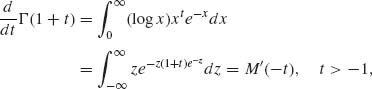
Let Iij, i = 1,2, j = 1,2 denote the elements of the Fisher information matrix. These elements are defined as
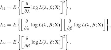
We will derive the formulae for these elements under the assumption of n = 1 observation. The resulting information matrix can then be multiplied by n to yield that of a random sample of size n. This is due to the fact that the random variables are i.i.d.
The partial derivatives of the log–likelihood are
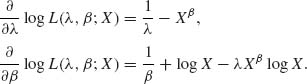
Thus,
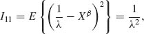
since Xβ ∼ E(λ). It is much more complicated to derive the other elements of I(θ). For this purpose, we introduce first a few auxiliary results. Let M(t) be the moment generating function of the extreme–value distribution. We note that
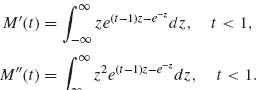
Accordingly,
similarly,
![]()
These identities are used in the following derivations:
where γ = 0.577216… is the Euler constant. Moreover, as compiled from the tables of Abramowitz and Stegun (1968, p. 253)
![]()
We also obtain
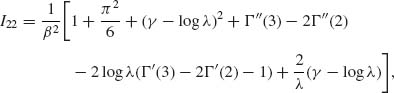
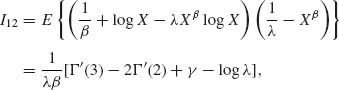
where Γ ″(2) = 0.82367 and Γ ″(3) = 2.49293. The derivations of formulae for I12 and I22 are lengthy and tedious. We provide here, for example, the derivation of one expectation:
![]()
However, Xβ ∼ E(λ) ∼ ![]() U, where U ∼ E(1). Therefore,
U, where U ∼ E(1). Therefore,
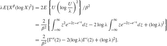
The reader can derive other expressions similarly.
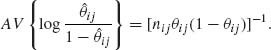
For each value of λ and β, we evaluate I11, I12, and I22. The asymptotic variances and covariances of the MLEs, designated by AV and AC, are determined from the inverse of the Fisher information matrix by
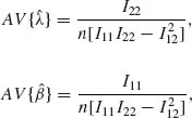
and
![]()
Applying these formulae to determine the asymptotic variances and asymptotic covariance of ![]() and
and ![]() of Example 5.20, we obtain, for λ = 1 and β = 1.75, the numerical results I11 = 1, I12 = 0.901272, and I22 = 1.625513. Thus, for n = 50, we have AV{
of Example 5.20, we obtain, for λ = 1 and β = 1.75, the numerical results I11 = 1, I12 = 0.901272, and I22 = 1.625513. Thus, for n = 50, we have AV{![]() } = 0.0246217, AV{
} = 0.0246217, AV{![]() } = 0.0275935 and AC(
} = 0.0275935 and AC(![]() ,
, ![]() ) = −0.0221655. The asymptotic standard errors (square roots of AV) of
) = −0.0221655. The asymptotic standard errors (square roots of AV) of ![]() and
and ![]() are, 0.1569 and 0.1568, respectively. Thus, the estimates
are, 0.1569 and 0.1568, respectively. Thus, the estimates ![]() = 0.839 and
= 0.839 and ![]() = 1.875 are not significantly different from the true values λ = 1 and β = 1.75.
= 1.875 are not significantly different from the true values λ = 1 and β = 1.75. ![]()
Example 7.8. Let X1, …, Xn be i.i.d. random variables with X1∼ E ![]() , 0 < ξ < ∞. Let Y1, …, Yn be i.i.d. random variables, Y1 ∼ G
, 0 < ξ < ∞. Let Y1, …, Yn be i.i.d. random variables, Y1 ∼ G ![]() , 0 < η < ∞, and assume that the Y–sample is independent of the X–sample.
, 0 < η < ∞, and assume that the Y–sample is independent of the X–sample.
The parameter to estimate is θ = ![]() . The MLE of θ is
. The MLE of θ is ![]() n =
n = ![]() , where
, where ![]() n and
n and ![]() n are the corresponding sample means. For each n ≥ 1,
n are the corresponding sample means. For each n ≥ 1, ![]() n ∼ θ F[2n, 2n]. The asymptotic distribution of
n ∼ θ F[2n, 2n]. The asymptotic distribution of ![]() n is N
n is N![]() , 0 < θ < ∞.
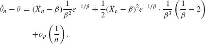
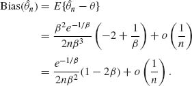
, 0 < θ < ∞. ![]() n is a BAN estimator. To find the asymptotic bias of
n is a BAN estimator. To find the asymptotic bias of ![]() n, verify that
n, verify that
The bias of the MLE is B(![]() n) =
n) = ![]() , which is of
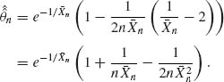
, which is of ![]() . Thus, we adjust
. Thus, we adjust ![]() n by
n by ![]() =
= ![]()
![]() n. The bias of
n. The bias of ![]() is B(
is B(![]() ) = 0. The variance of
) = 0. The variance of ![]() is
is
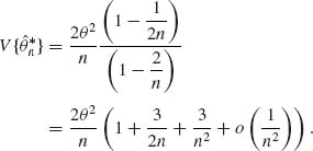
Thus, the second–order deficiency coefficients of ![]() is D = 3θ2. Note that
is D = 3θ2. Note that ![]() is the UMVU estimator of θ.
is the UMVU estimator of θ. ![]()
Example 7.9. Let X1, X2, …, Xn be i.i.d. Poisson random variables, with mean λ, 0 < λ < ∞. We consider θ = e−λ, 0 < θ < 1.
The UMVU of θ is
![]()
where Tn = ![]() Xi. The MLE of θ is
Xi. The MLE of θ is
![]()
where ![]() n = Tn/n. Note that
n = Tn/n. Note that ![]() n −
n − ![]() n
n ![]() 0. The two estimators are asymptotically equivalent. Using moment generating functions, we prove that
0. The two estimators are asymptotically equivalent. Using moment generating functions, we prove that
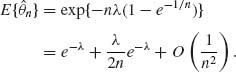
Thus, adjusting the MLE for the bias, let
![]()
Note that, by the delta method,
![]()
Thus,
![]()
The variance of the bias adjusted estimator ![]() is
is
![]()
Continuing the computations, we find
![]()
Similarly,
![]()
It follows that
![]()
In the present example, the bias adjusted MLE is most efficient second–order estimator. The variance of the UMVU ![]() n is
n is
![]()
Thus, ![]() n has the deficiency coefficient D = λ2 e−2λ/2.
n has the deficiency coefficient D = λ2 e−2λ/2.
Example 7.10
In the present case, θL = 0.462 and θU = 0.656. We can also, as mentioned earlier, determine the approximate confidence limits directly on θ by estimating the variance of θ. In this case, we obtain the limits
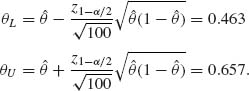
Both approaches yield here close results, since the sample is sufficiently large.
![]()
The MLE of ρ is the sample coefficient of correlation r = Σ (Xi − ![]() )(Yi −
)(Yi − ![]() )/[Σ (Xi −
)/[Σ (Xi − ![]() )2 · Σ (Yi −
)2 · Σ (Yi − ![]() )2]1/2. By determining the inverse of the Fisher information matrix one obtains that the asymptotic variance of r is AV{r} =
)2]1/2. By determining the inverse of the Fisher information matrix one obtains that the asymptotic variance of r is AV{r} = ![]() (1-ρ2)2. Thus, if we make the transformation g(ρ) =
(1-ρ2)2. Thus, if we make the transformation g(ρ) = ![]() log
log ![]() then g′(ρ) =
then g′(ρ) = ![]() . Thus, g(r) =
. Thus, g(r) = ![]() log ((1 + r)/(1 − r)) is a variance stabilizing transformation for r, with an asymptotic variance of 1/n. Suppose that in a sample of n = 100 we find a coefficient of correlation r = 0.79. Make the transformation
log ((1 + r)/(1 − r)) is a variance stabilizing transformation for r, with an asymptotic variance of 1/n. Suppose that in a sample of n = 100 we find a coefficient of correlation r = 0.79. Make the transformation
![]()
We obtain on the basis of this transformation the asymptotic limits
![]()
The inverse transformation is ρ = (e2g−1)/(e2g + 1). Thus, the confidence interval of ρ has the limits ρL = 0.704 and ρU = 0.853. On the other hand, if we use the formula
![]()
We obtain the limits ρL = 0.716 and ρU = 0.864. The two methods yield confidence intervals which are close, but not the same. A sample of size 100 is not large enough. ![]()
Example 7.11. In Example 6.6, we determined the confidence limits for the cross–ratio productρ. We develop here the large sample approximation, according to the two approaches discussed above. Let
![]()
Let ![]() ij = Xij/nij (i, j = 1,2).
ij = Xij/nij (i, j = 1,2). ![]() ij is the MLE of θij. Let
ij is the MLE of θij. Let ![]() ij = log (θij/(1 − θij)). The MLE of
ij = log (θij/(1 − θij)). The MLE of ![]() ij is
ij is ![]() ij = log (
ij = log (![]() ij/(1 −
ij/(1 − ![]() ij)). The asymptotic distribution of
ij)). The asymptotic distribution of ![]() ij is normal with mean
ij is normal with mean ![]() ij and
ij and
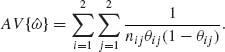
Furthermore, the MLE of ω is
![]()
Since Xij, (i, j) = 1,2, are mutually independent so are the terms on the RHS of ![]() . Accordingly, the asymptotic distribution of
. Accordingly, the asymptotic distribution of ![]() is normal with expectation ω and asymptotic variance
is normal with expectation ω and asymptotic variance
Since the values θij are unknown we substitute their MLEs. We thus define the standard error of ![]() as
as
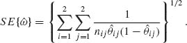
According to the asymptotic normal distribution of ![]() , the asymptotic confidence limits for ρ are
, the asymptotic confidence limits for ρ are
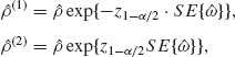
where ![]() is the MLE of ρ = eω. These limits can be easily computed. For a numerical example, consider the following table (Fleiss, 1973, p. 126) in which we present the proportions of patients diagnosed as schizophrenic in two studies both performed in New York and London.
is the MLE of ρ = eω. These limits can be easily computed. For a numerical example, consider the following table (Fleiss, 1973, p. 126) in which we present the proportions of patients diagnosed as schizophrenic in two studies both performed in New York and London.
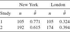
These samples yield the MLE ![]() = 2.9. The asymptotic confidence limits at level 1 − α = 0.95 are
= 2.9. The asymptotic confidence limits at level 1 − α = 0.95 are ![]() (1) = 1.38 and
(1) = 1.38 and ![]() (2) = 6.08. This result indicates that the interaction parameter ρ is significantly greater than 1. We show now the other approach, using the variance stabilizing transformation 2 sin −1(
(2) = 6.08. This result indicates that the interaction parameter ρ is significantly greater than 1. We show now the other approach, using the variance stabilizing transformation 2 sin −1(![]() ). Let
). Let ![]() ij = (Xij + 0.5)/(nij + 1) and Yij = 2 sin −1(
ij = (Xij + 0.5)/(nij + 1) and Yij = 2 sin −1(![]() ij). On the basis of these variables, we set the 1 − α confidence limits for ηij = 2 sin −1(
ij). On the basis of these variables, we set the 1 − α confidence limits for ηij = 2 sin −1(![]() ). These are
). These are
![]()
For these limits, we directly obtain the asymptotic confidence limits for ![]() ij that are
ij that are
![]()
where
![]()
and
![]()
We show now how to construct asymptotic confidence limits for ρ from these asymptotic confidence limits for ![]() ij.
ij.
Define
![]()
and
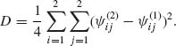
D is approximately equal to ![]() AV{
AV{![]() }. Indeed, from the asymptotic theory of MLEs,
}. Indeed, from the asymptotic theory of MLEs, ![]() /4 is approximately the asymptotic variance of
/4 is approximately the asymptotic variance of ![]() ij times
ij times ![]() . Accordingly,
. Accordingly,
![]()
and by employing the normal approximation, the asymptotic confidence limits for ρ are
![]()
Thus, we obtain the approximate confidence limits for Fleiss’ example, ρ(1) = 1.40 and ρ(2) = 6.25. These limits are close to the ones obtained by the other approach. For further details, see Zacks and Solomon (1976). ![]()
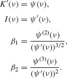
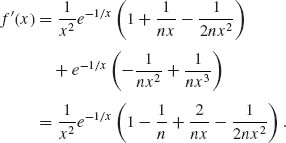
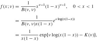
Example 7.12. Let X1, X2, …, Xn be i.i.d. random variables having the gamma distribution G(1,ν), 0 < ν < ∞. This is a one–parameter exponential type family, with canonical p.d.f.
![]()
Here, K(ν) = log Γ (ν).
The MLE of ν is the root of the equation

where ![]() n =
n = ![]()
![]() log (Xi). The function Γ′(ν)/Γ (ν) is known as the di–gamma, or psi function,
log (Xi). The function Γ′(ν)/Γ (ν) is known as the di–gamma, or psi function, ![]() (ν) (see Abramowitz and Stegun, 1968, p. 259).
(ν) (see Abramowitz and Stegun, 1968, p. 259). ![]() (ν) is tabulated for 1 ≤ ν ≤ 2 in increments of Δ = 0.05. For ν values smaller than 1 or greater than 2 use the recursive equation
(ν) is tabulated for 1 ≤ ν ≤ 2 in increments of Δ = 0.05. For ν values smaller than 1 or greater than 2 use the recursive equation
![]()
The values of ![]() n can be determined by numerical interpolation.
n can be determined by numerical interpolation.
The function ![]() (ν) is analytic on the complex plane, excluding the points ν = 0, −1, −2, …. The nth order derivative of
(ν) is analytic on the complex plane, excluding the points ν = 0, −1, −2, …. The nth order derivative of ![]() (ν) is
(ν) is
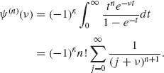
Accordingly,
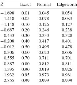
To assess the normal and the Edgeworth approximations to the distribution of ![]() n, we have simulated 1000 independent random samples of size n = 20 from the gamma distribution with ν = 1. In this case I(1) = 1.64493, β1 = −1.1395 and β2 − 3 = 2.4. In Table 7.1, we present some empirical quantiles of the simulations. We see that the Edgeworth approximation is better than the normal for all standardized values of
n, we have simulated 1000 independent random samples of size n = 20 from the gamma distribution with ν = 1. In this case I(1) = 1.64493, β1 = −1.1395 and β2 − 3 = 2.4. In Table 7.1, we present some empirical quantiles of the simulations. We see that the Edgeworth approximation is better than the normal for all standardized values of ![]() n between the 0.2th and 0.8th quantiles. In the tails of the distribution, one could get better results by the saddlepoint approximation.
n between the 0.2th and 0.8th quantiles. In the tails of the distribution, one could get better results by the saddlepoint approximation. ![]()
Table 7.1 Normal and Edgeworth Approximations to the Distribution of ![]() 20, n = 20, ν = 1
20, n = 20, ν = 1
Example 7.13. Let X1, X2, …, Xn be i.i.d. random variables having the exponential distribution X1 ∼ E(![]() ), 0 <
), 0 < ![]() < ∞. This is a one–parameter exponential family with canonical p.d.f.
< ∞. This is a one–parameter exponential family with canonical p.d.f.
![]()
where U(x) = −x and K(![]() ) = −log (
) = −log (![]() ).
).
The MLE of ![]() is
is ![]() n = 1/
n = 1/![]() n. The p.d.f. of
n. The p.d.f. of ![]() n is obtained from the density of
n is obtained from the density of ![]() n and is
n and is
![]()
for 0 < x < ∞.
The approximation to the p.d.f. according to (7.6.9) yields
Substituting cn = nne−n/Γ (n) we get the exact equation. ![]()
Example 7.14. Let X1, X2, …, Xn be i.i.d. random variables, having a common normal distribution N(θ, 1). Consider the problem of testing the hypothesis H0: θ ≤,0 against H1: θ > 0. We have seen that the uniformly most powerful (UMP) test of size α is
![]()
where ![]() n =
n = ![]()
![]() Xi and and Z1 − α = Φ −1 (1 − α). The power function of this UMP test is
Xi and and Z1 − α = Φ −1 (1 − α). The power function of this UMP test is
![]()
Let θ1 > 0 be specified. The number of observations required so that ![]() n(θ1) ≥ γ is
n(θ1) ≥ γ is
![]()
Note that
![]()
where 0 < α < ![]() ∞ < 1.
∞ < 1.
Suppose that one wishes to consider a more general model, in which the p.d.f. of X1 is f(x − θ), −∞ < θ < ∞, where f(x) is symmetric about θ but not necessarily equal to ![]() (x), and Vθ {X} = σ2 for all −∞ < θ < ∞. We consider the hypotheses H0: θ ≤ 0 against H1: θ > 0.
(x), and Vθ {X} = σ2 for all −∞ < θ < ∞. We consider the hypotheses H0: θ ≤ 0 against H1: θ > 0.
Due to the CLT, one can consider the sequence of test statistics
![]()
where an ![]() Z1 − α as n→ ∞, and the alternative sequence
Z1 − α as n→ ∞, and the alternative sequence
![]()
where Me is the sample median
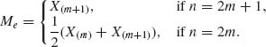
According to Theorem 1.13.7, ![]() (Me − θ)
(Me − θ) ![]() N
N ![]() as n→ ∞. Thus, the asymptotic power functions of these tests are
as n→ ∞. Thus, the asymptotic power functions of these tests are
![]()
and
![]()
Both ![]() (θ1) and
(θ1) and ![]() (θ1) converge to 1 as n→ ∞, for any θ1 > 0, which shows their consistency. We wish, however, to compare the behavior of the sequences of power functions for θn =
(θ1) converge to 1 as n→ ∞, for any θ1 > 0, which shows their consistency. We wish, however, to compare the behavior of the sequences of power functions for θn = ![]() . Note that each hypothesis, with θ1,n =
. Note that each hypothesis, with θ1,n = ![]() is an alternative one. But, since θ1,n → 0 as n→ ∞, these alternative hypotheses are called local hypotheses. Here we get
is an alternative one. But, since θ1,n → 0 as n→ ∞, these alternative hypotheses are called local hypotheses. Here we get
![]()
and
![]()
To insure that ![]() * =
* = ![]() ** one has to consider for
** one has to consider for ![]() (2) a sequence of alternatives
(2) a sequence of alternatives ![]() with sample size n′ =
with sample size n′ = ![]() so that
so that
![]()
The Pitman ARE of ![]() to
to ![]() is defined as the limit of n/n′(n) as n→ ∞. In the present example,
is defined as the limit of n/n′(n) as n→ ∞. In the present example,
![]()
If the original model of X∼ N(θ, 1), f(0) = ![]() and ARE of
and ARE of ![]() (2) to
(2) to ![]() (1) is 0.637. On the other hand, if f(x) =
(1) is 0.637. On the other hand, if f(x) = ![]() e−|x|, which is the Laplace distribution, then the ARE of
e−|x|, which is the Laplace distribution, then the ARE of ![]() (2) to
(2) to ![]() (1) is 1.
(1) is 1. ![]()
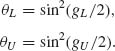
Example 7.15. In Example 7.3, we discussed the Wilcoxon signed–rank test of H0: θ ≤ θ0 versus H1: θ > θ0, when the distribution function F is absolutely continuous and symmetric around θ. We show here the Pitman’s asymptotic efficiency of this test relative to the t–test. The t–test is valid only in cases where ![]() = V{X} and 0 <
= V{X} and 0 < ![]() < ∞. The t–statistic is tn =
< ∞. The t–statistic is tn = ![]() , where
, where ![]() is the sample variance. Since Sn
is the sample variance. Since Sn ![]() σf, as n→ ∞, we consider
σf, as n→ ∞, we consider
![]()
The asymptotic efficacy of the t–test is
![]()
where ![]() is the variance of X, under the p.d.f. f(x). Indeed, μ (θ) = θ.
is the variance of X, under the p.d.f. f(x). Indeed, μ (θ) = θ.
Consider the Wilcoxon signed–rank statistic Tn, given by (7.1.3). The test function, for large n, is given by (7.1.8). For this test
![]()
where p2(θ) is given in Example 7.3. Thus,
![]()
Hence,
![]()
Using σ2(0) = ![]() , we obtain the asymptotic efficacy of
, we obtain the asymptotic efficacy of
![]()
as n→ ∞. Thus, the Pitman ARE of Tn versus tn is
(7.9.16) ![]()
Thus, if f(x) = ![]() (x) (standard normal) ARE (Tn, tn) = 0.9549. On the other hand, if f(x) =
(x) (standard normal) ARE (Tn, tn) = 0.9549. On the other hand, if f(x) = ![]() exp {−|x|} (standard Laplace) then ARE (Tn, tn) = 1.5. These results deem the Wilcoxon signed–rank test to be asymptotically very efficient nonparametric test.
exp {−|x|} (standard Laplace) then ARE (Tn, tn) = 1.5. These results deem the Wilcoxon signed–rank test to be asymptotically very efficient nonparametric test. ![]()
Example 7.16. Let X1, …, Xn be i.i.d. random variables, having a common Cauchy distribution, with a location parameter θ, −∞ < θ < ∞, i.e.,
![]()
We derive a confidence interval for θ, for large n (asymptotic). Let ![]() n be the sample median, i.e.,
n be the sample median, i.e.,
![]()
Note that, due to the symmetry of f(x;θ) around θ, θ = F−1![]() . Moreover,
. Moreover,
![]()
Hence, the (1 − α) confidence limits for θ are
![]()
![]()
PART III: PROBLEMS
Section 7.1
7.1.1 Let Xi = α + β zi + ![]() i, i = 1, …,n, be a simple linear regression model, where z1, …,zn are prescribed constants, and
i, i = 1, …,n, be a simple linear regression model, where z1, …,zn are prescribed constants, and ![]() 1, …,
1, …, ![]() n are independent random variables with E{ei} = 0 and V{
n are independent random variables with E{ei} = 0 and V{![]() i} = σ2, 0 < σ2 < ∞, for all i = 1, …,n. Let
i} = σ2, 0 < σ2 < ∞, for all i = 1, …,n. Let ![]() and
and ![]() n be the LSE of α and β.
n be the LSE of α and β.
7.1.2 Suppose that X1, X2, …, Xn, … are i.i.d. random variables and 0 < E{![]() } < ∞. Give a strongly consistent estimator of the kurtosis coefficient β2 =
} < ∞. Give a strongly consistent estimator of the kurtosis coefficient β2 = ![]() .
.
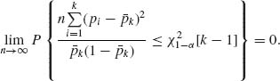
7.1.3 Let X1, …, Xk be independent random variables having binomial distributions B(n, θi), i = 1, …, k. Consider the null hypothesis H0: θ1 = ··· = θk against the alternative H1: ![]() (θi −
(θi − ![]() )2 > 0, where
)2 > 0, where ![]() =
= ![]() θi. Let pi = Xi/n and
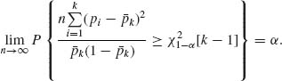
θi. Let pi = Xi/n and  . Show that the test function
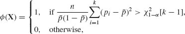
has a size αn converging to α as n→ ∞. Show that this test is consistent.
7.1.4 In continuation of Problem 3, define Yi = 2 sin −1![]() , i = 1, …, k.
, i = 1, …, k.
Section 7.2
7.2.1 Let X1, X2, …, Xn, … be i.i.d. random variables, X1 ∼ G(1,ν), 0 < ν ≤ ν* < ∞. Show that all conditions of Theorem 7.2.1 are satisfied, and hence the MLE, ![]() n
n ![]() ν as n→ ∞ (strongly consistent).
ν as n→ ∞ (strongly consistent).
7.2.2 Let X1, X2, …, Xn, … be i.i.d. random variables, X1∼ β (ν, 1), 0 < ν < ∞. Show that the MLE, ![]() n, is strongly consistent.
n, is strongly consistent.
7.2.3 Consider the Hardy–Weinberg genetic model, in which (J1, J2) ∼ MN(n,(p1(θ),p2(θ))), where p1(θ) = θ2 and p2(θ) = 2θ (1 − θ), 0 < θ < 1. Show that the MLE of θ, ![]() n, is strongly consistent.
n, is strongly consistent.
7.2.4 Let X1, X2, …, Xn be i.i.d. random variables from G(λ, 1), 0 < λ < ∞. Show that the following estimators ![]() (
(![]() n) are consistent estimators of ω (λ):
n) are consistent estimators of ω (λ):
7.2.5 Let X1, …, Xn be i.i.d. from N(μ, σ2), −∞ < μ < ∞, 0 < σ < ∞. Show that
Section 7.3
7.3.1 Let (Xi, Yi), i = 1, …,n be i.i.d. random vectors, where
![]()
−∞ < ξ < ∞, 0 < η < ∞, 0 < σ1, σ2 < ∞, −1 < ρ < 1. Find the asymptotic distribution of Wn = ![]() n/
n/ ![]() n, where
n, where ![]() n =
n = ![]()
![]() Xi and
Xi and ![]() n =
n = ![]()
![]() Yi.
Yi.
7.3.2 Let X1, X2, …, Xn, … be i.i.d. random variables having a Cauchy distribution with location parameter θ, i.e.,
![]()
Let Me be the sample median, or Me = ![]()
![]() . Is Me a BAN estimator?
. Is Me a BAN estimator?
7.3.3 Derive the asymptotic variances of the MLEs of Problems 1–3 of Section 5.6 and compare the results with the large sample approximations of Problem 4 of Section 5.6.
7.3.4 Let X1, …, Xn be i.i.d. random variables. The distribution of X1 as that of N(μ, σ2). Derive the asymptotic variance of the MLE of Φ(μ /σ).
7.3.5 Let X1, …, Xn be i.i.d. random variables having a log–normal distribution LN(μ, σ2). What is the asymptotic covariance matrix of the MLE of ξ = exp {μ + σ2/2} and D2 = ξ2 exp {σ2 − 1}?
Section 7.4
7.4.1 Let X1, X2, …, Xn be i.i.d. random variables having a normal distribution N(μ, σ2), −∞ < μ < ∞, 0 < σ < ∞. Let θ = eμ.
7.4.2 Let X1, X2, …, Xn be i.i.d. random variables, X1 ∼ G![]() , 0 < β < ∞. Let θ = e−1/β, 0 < θ < 1.
, 0 < β < ∞. Let θ = e−1/β, 0 < θ < 1.
7.4.3 Let X1, X2, …, Xn be i.i.d. random variables having a one–parameter canonical exponential type p.d.f. Show that the first order bias term of the MLE ![]() n is
n is
![]()
Section 7.5
7.5.1 In a random sample of size n = 50 of random vectors (X, Y) from a bivariate normal distribution, −∞ < μ, η < ∞, 0 < σ1, σ2 < ∞, −1 < ρ < 1, the MLE of ρ is ![]() = 0.85. Apply the variance stabilizing transformation to determine asymptotic confidence limits of
= 0.85. Apply the variance stabilizing transformation to determine asymptotic confidence limits of ![]() = sin −1(ρ); −
= sin −1(ρ); −![]() <
< ![]() <
< ![]() .
.
7.5.2 Let ![]() be the sample variance in a random sample from a normal distribution N(μ, σ2). Show that the asymptotic variance of
be the sample variance in a random sample from a normal distribution N(μ, σ2). Show that the asymptotic variance of
![]()
Suppose that n = 250 and ![]() = 17.39. Apply the above transformation to determine asymptotic confidence limits, at level 1 − α = 0.95, for σ2.
= 17.39. Apply the above transformation to determine asymptotic confidence limits, at level 1 − α = 0.95, for σ2.
7.5.3 Let X1, …, Xn be a random sample (i.i.d.) from N(μ, σ2); −∞ < μ < ∞, 0 < σ2 < ∞.
7.5.4 Let X1, …, Xn be a random sample from a location parameter Laplace distribution; −∞ < μ < ∞. Determine a (1 − α)–level asymptotic confidence interval for μ.
Section 7.6
7.6.1 Let X1, X2, …, Xn be i.i.d. random variables having a one–parameter Beta (ν, ν) distribution.
7.6.2 In continuation of the previous problem, derive the p*–formula of the density of the MLE, ![]() n?
n?
PART IV: SOLUTION OF SELECTED PROBLEMS
7.1.3 Let θ′ = (θ1, …, θk) and p′ = (p1, …, pk). Let D = (diag(θi(1 − θi)), i = 1, …,k) be a k × k diagonal matrix. Generally, we denote Xn ∼ AN ![]() if
if ![]() (Xn − ξ)
(Xn − ξ) ![]() N(0, V) as n→ ∞. [AN(·, ·) stands for ‘asymptotically normal’]. In the present case,
N(0, V) as n→ ∞. [AN(·, ·) stands for ‘asymptotically normal’]. In the present case, ![]() .
.
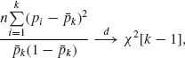
Let H0: θ1 = θ2 = ··· =θk = θ. Then, if H0 is true,
![]()
Now, ![]() (pi −
(pi − ![]() k)2 = p′
k)2 = p′ ![]() p, where Jk = 1k1′k. Since
p, where Jk = 1k1′k. Since ![]() is idempotent, of rank (k−1), np′
is idempotent, of rank (k−1), np′![]() p
p ![]() θ (1 − θ)χ2[k−1]. Moreover,
θ (1 − θ)χ2[k−1]. Moreover, ![]() k =
k = ![]() pi → θ a.s., as n→ ∞. Thus, by Slutsky’s Theorem
pi → θ a.s., as n→ ∞. Thus, by Slutsky’s Theorem
and
If H0 is not true, ![]() (θi −
(θi − ![]() k)2 > 0. Also,
k)2 > 0. Also,
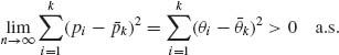
Thus, under H1,
Thus, the test is consistent.
7.2.3 The MLE of θ is ![]() n =
n =![]() . J1∼ B(n, θ2). Hence,
. J1∼ B(n, θ2). Hence, ![]() and
and ![]() . Thus,
. Thus, ![]()
![]() n = θ a.s.
n = θ a.s.
7.3.1 By SLLN, ![]() a.s.
a.s.
![]()
where
![]()
Thus, ![]() .
.
7.3.2 As shown in Example 7.16,
![]()
Also,
![]()
On the other hand, the Fisher information is In(θ) = ![]() . Thus, AV(
. Thus, AV(![]() n) =
n) = ![]() . Thus,
. Thus, ![]() n is not a BAN estimator.
n is not a BAN estimator.
7.4.2
Hence,
The bias adjusted estimator is
It follows that
![]()
Accordingly, the second–order deficiency coefficient of ![]() n is
n is
![]()
7.6.1 X1, …, Xn are i.i.d. like Beta (ν, ν), 0 < ν < ∞.
where K(ν) = log B(ν, ν).
The log likelihood is
![]()
Note that the derivative of K(ν) is
![]()
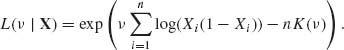
It follows that the MLE of ν is the root of
![]()
The function ![]() log Γ (ν) is also called the psi function, i.e.,
log Γ (ν) is also called the psi function, i.e., ![]() (ν) =
(ν) = ![]() log Γ (ν). As shown in Abramowitz and Stegun (1968, p. 259),
log Γ (ν). As shown in Abramowitz and Stegun (1968, p. 259), ![]() (2ν) −
(2ν) − ![]() (ν) =
(ν) = ![]() (
(![]()
![]() −
− ![]() (ν))+log 2. Also, −
(ν))+log 2. Also, −![]()
![]() log (Xi(1 − Xi)) > log 4. Thus, the MLE is the value of ν for which
log (Xi(1 − Xi)) > log 4. Thus, the MLE is the value of ν for which
![]()
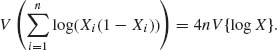
Thus, since X1, …, Xn are i.i.d., the Fisher information is I(ν) = 4V{log X}. The first four central moments of Beta (ν, ν) are ![]() = 0;
= 0; ![]() =
= ![]() ;
; ![]() = 0 and
= 0 and ![]() . Thus,
. Thus,
![]()
and
![]()
It follows that the Edgeworth asymptotic approximation to the distribution of the MLE, ![]() n, is
n, is
![]()