Chapter 17

Implementing Laplace Techniques for Circuit Analysis

In This Chapter

Starting with basic constraints in the s-domain

Looking at voltage and current divider techniques in the s-domain

Using superposition, Thévenin, Norton, node voltages, and mesh currents in the s-domain

This chapter is all about applying Laplace transform techniques in order to study circuits that have voltage and current signals changing with time. That may sound complex, but it’s really no more difficult than analyzing resistor-only circuits. You see, the Laplace method converts a circuit to the s-domain so you can study the circuit’s action using only algebraic techniques (rather than the calculus techniques I show you in Chapters 13 and 14). The algebraic approach in the s-domain follows along the same lines as resistor-only circuits, except in place of resistors, you have s-domain impedances.

If you need a refresher on impedance or the Laplace transform in general, see Chapters 15 and 16, respectively. Otherwise, I invite you to dive into this chapter, which first has you describe the element and connection constraints in the s-domain. You then see how the s-domain approach works when you apply voltage and current divider methods, Thévenin and Norton equivalents, node-voltage analysis, and mesh-current analysis.

Starting Easy with Basic Constraints

Connection constraints are those physical laws that cause element voltages and currents to behave in certain ways when the devices are interconnected to form a circuit. You also have constraints on the individual devices themselves, where each device has a mathematical relationship between the voltage across the device and the current through the device. The following sections show you what connection constraints, device constraints, impedances, and admittances wind up looking like in the s-domain.

Connection constraints in the s-domain

Transforming the connection constraints to the s-domain is a piece of cake. Kirchhoff’s current law (KCL) says the sum of the incoming and outgoing currents is equal to 0. Here’s a typical KCL equation described in the time-domain:

Because of the linearity property of the Laplace transform (Chapter 16), the KCL equation in the s-domain becomes the following:

You transform Kirchhoff’s voltage law (KVL) in the same way. KVL says the sum of the voltage rises and drops is equal to 0. Here’s a classic KVL equation described in the time-domain:

Because of linearity, the KVL equation in the s-domain produces

The basic form of KVL remains the same. Piece of cake!

Device constraints in the s-domain

You can easily transform the i-v constraints of devices such as independent and dependent sources, op amps, resistors, capacitors, and inductors to algebraic equations in the s-domain. After converting the device constraints, all you need is algebra. I show you how to translate current and voltage relationships to the s-domain in the following sections.

Independent and dependent sources

Transforming independent sources is a no-brainer because the s-domain has the same form as the time-domain:

Converting dependent sources is easy, too. Here are the equations for voltage-controlled voltage sources (VCVS), voltage-controlled current sources (VCCS), current-controlled voltage sources (CCVS), and current-controlled current sources (CCCS):

The constants μ, g, r, and β relate the dependent output sources V2(s) and I2(s) controlled by input variables V1(s) and I1(s). (For more information on dependent sources, see Chapter 9.)

Passive elements: Resistors, capacitors, and inductors

For resistors, capacitors, and inductors, you convert their i-v relationships to the s-domain using Laplace transform properties, such as the integration and derivative properties (which you find in Chapter 16):

The preceding three equations on the right are s-domain models that use voltage sources for the initial capacitor voltage vC(0) and initial inductor current iL(0).

You can rewrite these equations in the s-domain to model the initial conditions, vC(0) and iL(0), as current sources:

You see there are no integrals or derivatives in the s-domain.

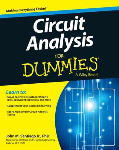
The middle column of Figure 17-1 shows the constraints of the passive devices in the time-domain being converted to the s-domain. The left column shows initial conditions modeled as voltage sources in the s-domain, and the right column shows initial conditions modeled as current sources in the s-domain.

Taking the initial conditions into account in the s-domain analysis for capacitors and inductors is a big deal because it expedites the analysis. When you transform differential equations into the s-domain, you deal with input sources and initial conditions simultaneously.

Illustration by Wiley, Composition Services Graphics

Figure 17-1: The s-domain models of passive devices.

Op-amp devices

The constraints of ideal operational amplifiers are unchanged in form in the s-domain:

Impedance and admittance

Impedance Z (see Chapter 15) relates the voltage and current described in the s-domain when initial conditions are set to 0. The following algebraic form of the i-v relationship describes impedance in the s-domain:

Admittance Y is the reciprocal of the impedance; it’s useful when you’re analyzing parallel circuits:

In the s-domain for zero initial conditions, the element constraints, impedances Z(s), and admittances Y(s) for the passive devices are as follows:

Now you’re ready to start analyzing circuits in the s-domain — without having to rely on calculus.

Seeing How Basic Circuit Analysis Works in the s-Domain

Circuit analysis techniques in the s-domain are powerful because you can treat a circuit that has voltage and current signals changing with time as though it were a resistor-only circuit. That means you can analyze the circuit algebraically, without having to mess with integrals and derivatives. In the following sections, you see how to apply voltage and current divider methods in the s-domain.

Applying voltage division with series circuits

You can put voltage divider techniques to work when dealing with series circuits, as Chapter 4 explains. To use voltage division in the s-domain, you simply replace the resistors with the impedances of devices connected in series. The following voltage divider equation is for three passive devices in a series circuit:

The output voltage V1(s) is based on the voltage source VS(s) and on the ratio of the desired impedance Z1(s) to the total impedance.

Figure 17-2 illustrates the voltage divider for a series circuit for zero initial conditions: iL(0) = 0 and vC(0) = 0. You can find the output transform of the capacitor voltage using the voltage divider equation:

In a similar way, the voltage transform across the inductor is

Illustration by Wiley, Composition Services Graphics

Figure 17-2: A series circuit and the voltage divider technique in the s-domain.

And the voltage transform across the resistor is

That’s all there is to it. You may need to do more algebraic gymnastics to simplify other circuits, but you still don’t need calculus. To get back to a time-domain description, you need to do a partial fraction expansion; then you look up the inverse Laplace transforms in the table in Chapter 16.

In many cases, you just want to predict what the output is when you’re given a particular input. When you know the transfer function, which is the ratio between the output transform and the input transform, you can multiply the transfer function by the input voltage to find the output. As a result, you can rewrite the transform of the capacitor voltage as a ratio of polynomials:

The denominator is simply a quadratic equation, and the roots of the equation shape the circuit behavior.

Similarly, you can rewrite the transform of the resistor and inductor voltages as a ratio of polynomials.

Turning to current division for parallel circuits

To use current division for parallel circuits having passive devices, all you have to do in the s-domain is replace the conductances with admittances. The following current divider equation is for three passive devices connected in parallel:

The output current I1(s) is based on the current source IS(s) and the ratio of the desired admittance Y1(s) to the total admittance.

Figure 17-3 illustrates the current divider technique for a parallel circuit for zero initial conditions: iL(0) = 0 and vC(0) = 0. You can find the output transform of the inductor current using the current divider equation:

Illustration by Wiley, Composition Services Graphics

Figure 17-3: Parallel circuits and the current divider technique in the s-domain.

In the same way, you get the transform of the capacitor and conductance (or resistor) currents using the current divider technique:

Note that the results resemble the form for series circuits using voltage divider techniques. Neat and simple in the s-domain — thank you, Pierre Laplace!

Conducting Complex Circuit Analysis in the s-Domain

In the time-domain, analyzing circuits with resistors, inductors, and capacitors involves integrals and derivatives. You use a simpler algebraic approach by describing and analyzing such circuits in the s-domain, as I show you next. The following sections cover node-voltage analysis, mesh-current analysis, superposition, and Norton and Thévenin equivalents in the s-domain.

Using node-voltage analysis

In the s-domain, node-voltage analysis works the same way as it does for resistor-only circuits, but this time you replace a device with its impedance. Node-voltage analysis (see Chapter 5) allows you to work with a smaller set of equations and unknowns that you need to deal with simultaneously. The unknown variables are called node voltages. After you find the unknown voltages, you can find the voltages and currents for each device.

Look at Figure 17-4, which shows a circuit at zero state using an op amp, resistor, and capacitor. You need to find the transfer function VO(s)/VS(s). Applying KCL at Node A produces the following:

Illustration by Wiley, Composition Services Graphics

Figure 17-4: Op-amp node-voltage analysis in the s-domain.

For an ideal op amp, IN = 0 and VN = VP = 0 because VP is connected to ground. The KCL equation becomes

After some algebra, you have the transfer function VO(s)/VS(s):

If the input is a step input u(t) and its transform is VS(s) = 1/s, the output transform becomes

Use the table in Chapter 16 to get the inverse Laplace transform:

The output vO(t) is a combination of a ramp and a step input. You get this when the circuit acts like an inverting amplifier and an integrator. You have a ramp resulting from the integration of a step input. The inverting amplifier comes into play when the capacitor acts like a short circuit, which occurs at high frequencies for sinusoidal inputs.

Using mesh-current analysis

Mesh-current analysis (see Chapter 6), which is useful when a circuit has several loops, works the same way in the s-domain as it does in resistor-only circuits. You simply use a device’s impedance to work the problem. After you solve for the mesh currents, you can find the voltage and current for each device.

Consider the circuit in Figure 17-5. You want to formulate the mesh current equation and solve for the zero-input and zero-state responses. The circuit is transformed into the s-domain.

For mesh-current analysis, you need to use the voltage source model of initial conditions; this will give you a circuit with voltage sources. You have the following mesh equations for Loops A and B:

Illustration by Wiley, Composition Services Graphics

Figure 17-5: Mesh-current analysis in the s-domain.

The matrix software should give you the following result, the algebraic equivalent for IB(s):

Using superposition and proportionality

The superposition concept basically says you can take an output v as a combination of weighted inputs. When applied to resistor circuits, the superposition concept (presented in Chapter 7) is described as

You can apply the same concept to linear circuits in the s-domain just by replacing the weighted constants with rational functions of s. Then you can look for the response as a sum of the zero-input response due to initial conditions with inputs turned off and the zero-state response due to external sources (inputs) with initial conditions turned off, which means no energy is stored. (You can review these two concepts in Chapters 13 and 14.) You turn off voltage sources by replacing them with short circuits and turn off current sources by replacing them with open circuits.

To see how to use superposition in the s-domain, check out Figure 17-6 where vs(t) is a step input u(t). The upper-left diagram describes an RC series circuit in the time domain, and the bottom-left diagram shows the same circuit described in the s-domain. I use this example to kill two birds with one stone: I apply superposition to find the zero-state VZS(s) or IZS(s) and the zero-input VZI(s) or IZI(s) transform responses, and I show you how to solve the problem by converting a differential equation or integral equation into the Laplace transform.

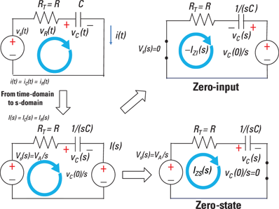
Illustration by Wiley, Composition Services Graphics

Figure 17-6: Zero-state and zero-input transforms using superposition.

First, you need to turn off the input source by replacing the voltage source with a short circuit, as the top-right diagram in Figure 17-6 shows. The result is the zero-input response:

The minus sign appears because the current is opposite to the assigned current direction in Figure 17-6. The pole at s = –1/(RC) comes from the circuit. Next, you need to turn off the initial condition modeled as a voltage source by replacing it with a short circuit. You see the zero-state diagram in the lower right of Figure 17-6. You now have the zero-state response for a step input:

The pole for the zero-state response is s = –1/(RC) from the circuit. Now use superposition to get the total response. Superposition says the total response is the sum of the zero-state and zero-input outputs:

The table in Chapter 16 tells you that the inverse Laplace transform is an exponential. The inverse Laplace transform of I(s) gives you the time response i(t):

This Laplace stuff really works! Calculus doesn’t come into play at all — all you need to do is look up transform pairs in a table to get the time response.

Now take a look at the lower-right circuit in Figure 17-6, which describes the circuit in zero-state in the s-domain. The differential equation for this circuit is based on KVL, given the capacitor voltage as an output variable and replacing forcing function vT(t) with a step input VAu(t):

Taking the Laplace transform of this equation gives you

Solve for the transform of the capacitor voltage VC(s):

The preceding equation shows you how the forcing function VAu(t) and the initial condition vC(0) are taken into account with one step based on the s-domain techniques. Performing a partial fraction expansion on the preceding equation gives you

Now take the inverse Laplace transform using the table in Chapter 16 to get the capacitor voltage response vC(t) in the time-domain:

Taking the derivative of vC(t) leads you to the capacitor current:

You get the same capacitor current iC(t), whether you transform the circuit or transform the differential equation. If you don’t like to take the derivative, you can start describing the circuit as an integral equation that just involves the capacitor current iC(t).

If you use the capacitor current iC(t) as the output variable, then the KVL equation becomes

Next, perform a Laplace transformation of the preceding equation:

Solve for the capacitor current IC(s):

Again, see how the forcing transform VA(s) and initial condition vC(0) are neatly separated components for the capacitor current IC(s).

Finally, take the inverse Laplace transform of the preceding equation:

Using the Thévenin and Norton equivalents

The Thévenin equivalent I present in Chapter 8 simplifies a circuit to one voltage source vT (t) and one single resistor RT. Extending the concept to circuits described in the s-domain means replacing the Thévenin resistance RT with an impedance ZT(s).

Similarly, the Norton equivalent replaces a complex circuit with a single current source iN(t) in parallel with the Norton resistor RN = RT. Extending the Norton concept to the s-domain means replacing the Norton resistance RN with the impedance ZN(s) = ZT(s). Figure 17-7 gives you the visual of how the Thévenin and Norton equivalents reduce circuits in the s-domain.

Illustration by Wiley, Composition Services Graphics

Figure 17-7: The s-domain Thévenin and Norton equivalents.

Take a look at the circuit in its zero state in Figure 17-8. The Thévenin and Norton equivalents are related by a source transformation, so use a source transformation to the left of Points A and B. The source transformation converts the Norton source circuit consisting of the independent current source IN = I1(s) in parallel with an impedance ZN = R to a Thévenin equivalent. The Thévenin equivalent consists of a voltage source VT = INZN = RI1(s) in series with ZT = ZN = R.

Illustration by Wiley, Composition Services Graphics

Figure 17-8: The s-domain source transformation and Thévenin equivalent.

You use voltage division to find the relationship between the output V2(s) and the input I1(s) in the s-domain:

Factoring out the coefficient LC in the denominator gives you

To emphasize the Thévenin equivalent when you have circuits with capacitors and inductors, take a look at the bottom diagram of Figure 17-8. The equivalent Thévenin impedance looking to the left from the capacitor terminals is simply the series connection of resistor R and the inductor impedance sL (or mathematically, ZT = R + sL).