Chapter 19: Sharing Your Work with the Outside World

In This Chapter

• Controlling access to your dashboards and reports

• Displaying your Excel dashboards in PowerPoint

• Saving your dashboards and reports to a PDF file

• Saving your dashboards to the web

The focus of this chapter is preparing your dashboard for life outside your PC. Here, we discuss the various methods of protecting your work from accidental and purposeful meddling and discover how you can distribute your dashboards via PowerPoint and PDF files.

Securing Your Dashboards and Reports

Before distributing any Excel-based work, always consider protecting your file by using the security capabilities native to Excel. Although none of Excel’s protection methods is hacker-proof, they do serve to protect the formulas, data structures, and other objects that make your dashboard tick.

Securing access to the entire workbook

Perhaps the best way to protect your Excel file is to use Excel’s protection options for file sharing. These options enable you to apply security at the workbook level, requiring a password to view or make changes to the file. This method is by far the easiest to apply and manage because there’s no need to protect each worksheet one at a time. You can apply a blanket protection to guard against unauthorized access and edits. Take a moment to review the file-sharing options, which are as follows:

→ Forcing read-only access to a file until a password is given

→ Requiring a password to open an Excel file

→ Removing workbook-level protection

The next few sections discuss these options in detail.

Permitting read-only access unless a password is given

You can force your workbook to go into read-only mode until the user types the password. This way, you can keep your file safe from unauthorized changes yet still allow authorized users to edit the file.

Here are the steps to force read-only mode:

1. With your file open, click the File tab.

2. To open the Save As dialog box, select Save As and then double-click the Computer icon.

3. In the Save As dialog box, click the Tools button and select General Options (see Figure 19-1).

The General Options dialog box appears.

4. Type an appropriate password in the Password to Modify input box (see Figure 19-2) and click OK.

5. Excel asks you to reenter your password, so reenter your chosen password.

6. Save your file to a new name.

At this point, your file is password protected from unauthorized changes. If you were to open your file, you’d see something similar to Figure 19-3. Failing to type the correct password causes the file to go into read-only mode.

Figure 19-1: The File Sharing options are well hidden away in the Save As dialog box under General Options.

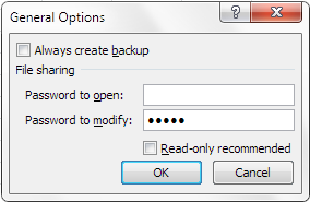
Figure 19-2: Type the password needed to modify the file.

Figure 19-3: A password is now needed to make changes to the file.

Note that Excel passwords are case-sensitive, so make sure Caps Lock on your keyboard is in the off position when entering your password.

Requiring a password to open an Excel file

You may have instances where your Excel dashboards are so sensitive only certain users are authorized to see them. In these cases, you can require your workbook to receive a password to open it. Here are the steps to set up a password for the file:

1. With your file open, click the File tab.

2. To open the Save As dialog box, select Save As and then double-click the Computer icon.

3. In the Save As dialog box, click the Tools button and select General Options (refer to Figure 19-1).

The General Options dialog box opens.

4. Type an appropriate password in the Password to Open text box (as shown in Figure 19-4) and click OK.

5. Excel asks you to reenter your password.

6. Save your file to a new name.

At this point, your file is password protected from unauthorized viewing.

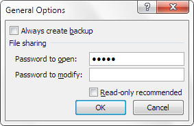
Figure 19-4: Type the password needed to modify the file.

Removing workbook-level protection

Removing workbook-level protection is as easy as clearing the passwords from the General Options dialog box. Here’s how you do it:

1. With your file open, click the File tab.

2. To open the Save As dialog box, select Save As.

3. In the Save As dialog box, click the Tools button and select General Options (refer to Figure 19-1).

The General Options dialog box opens.

4. Clear the Password to Open input box as well as the Password to Modify input box and click OK.

5. Save your file.

When you select the Read-Only Recommended check box in the General Options dialog box (refer to Figure 19-4), you get a cute but useless message recommending read-only access upon opening the file. This message is only a recommendation and doesn’t prevent anyone from opening the file as read/write.

Limiting access to specific worksheet ranges

You may find that you need to lock specific worksheet ranges, preventing users from taking certain actions. For example, you may not want users to break your data model by inserting or deleting columns and rows. You can prevent this by locking those columns and rows.

Unlocking editable ranges

By default, all cells in a worksheet are set to be locked when you apply worksheet-level protection. The cells on that worksheet can’t be altered in any way. That being said, you may find you need certain cells or ranges to be editable even in a locked state, like the example shown in Figure 19-5.

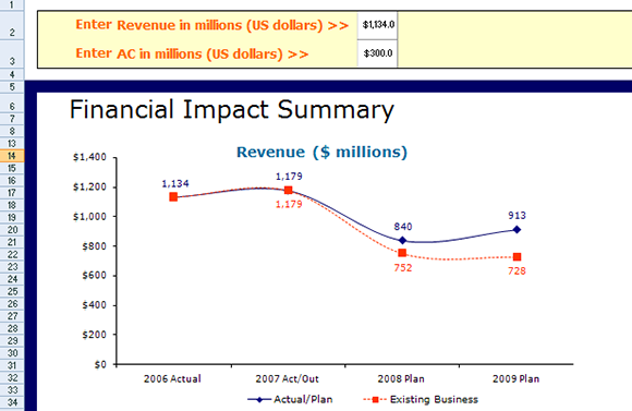
Figure 19-5: Though this sheet is protected, users can enter 2006 data into the input cells provided.

Before you protect your worksheet, you can unlock the cell or range of cells that you want users to be able to edit. (The next section shows you how to protect your entire worksheet.) Here’s how to do it:

1. Select the cells you need to unlock.

2. Right-click and select Format Cells.

3. On the Protection tab, as shown in Figure 19-6, deselect the Locked check box.

4. Click OK to apply the change.

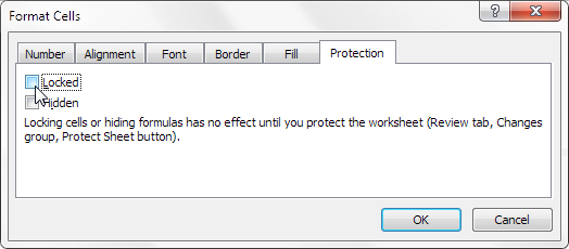
Figure 19-6: To ensure that a cell remains unlocked when the worksheet is protected, deselect the Locked check box.

Applying worksheet protection

After you’ve selectively unlocked the necessary cells, you can begin to apply worksheet protection. Just follow these steps:

1. To open the Protect Sheet dialog box, click the Protect Sheet icon on the Review tab of the Ribbon (see Figure 19-7).

2. Type a password in the text box (see Figure 19-8) and then click OK.

This is the password that removes worksheet protection. Note that because you can apply and remove worksheet protection without a password, specifying one is optional.

3. In the list box (see Figure 19-8), select which elements users can change after you protect the worksheet.

When a check box is cleared for a particular action, Excel prevents users from taking that action.

4. If you provided a password, reenter the password.

5. Click OK to apply the worksheet protection.

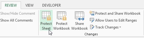
Figure 19-7: Select Protect Sheet in the Review tab.

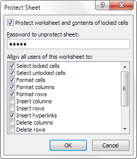
Figure 19-8: Specify a password that removes worksheet protection.

Removing worksheet protection

Just follow these steps to remove any worksheet protection you may have applied:

1. Click the Unprotect Sheet icon on the Review tab.

2. If you specified a password while protecting the worksheet, Excel asks you for that password (see Figure 19-9). Type the password and click OK to immediately remove protection.

Figure 19-9: The Unprotect Sheet icon removes worksheet protection.

Protecting the workbook structure

If you look under the Review tab in the Ribbon, you see the Protect Workbook icon next to the Protect Sheet icon. Protecting the workbook enables you to prevent users from taking any action that affects the structure of your workbook, such as adding/deleting worksheets, hiding/unhiding worksheets, and naming or moving worksheets. Just follow these steps to protect a workbook:

1. To open the Protect Structure and Windows dialog box, click the Protect Workbook icon on the Review tab of the Ribbon, as shown in Figure 19-10.

2. Choose which elements you want to protect: workbook structure, windows, or both. When a check box is cleared for a particular action, Excel prevents users from taking that action.

3. If you provided a password, reenter the password.

4. Click OK to apply the worksheet protection.

Figure 19-10: The Protect Structure and Windows dialog box.

Selecting Structure prevents users from doing the following:

→ Viewing worksheets that you’ve hidden

→ Moving, deleting, hiding, or changing the names of worksheets

→ Inserting new worksheets or chart sheets

→ Moving or copying worksheets to another workbook

→ Displaying the source data for a cell in a pivot table Values area or displaying pivot table Filter pages on separate worksheets

→ Creating a scenario summary report

→ Using an Analysis ToolPak utility that requires results to be placed on a new worksheet

→ Recording new macros

Choosing Windows prevents users from changing, moving, or sizing the workbook windows while the workbook is opened.

Linking Your Excel Dashboards to PowerPoint

You may find that your organization heavily favors PowerPoint presentations for periodic updates. Several methods exist for linking your Excel dashboards to a PowerPoint presentation. For current purposes, we focus on the method that is most conducive to presenting frequently updated dashboards and reports in PowerPoint — creating a dynamic link. A dynamic link allows your PowerPoint presentation to automatically pick up changes that you make to data in your Excel worksheet.

This technique of linking Excel charts to PowerPoint is ideal if you aren’t proficient at building charts in PowerPoint. Build the chart in Excel and then create a link for the chart in PowerPoint.

Creating the link between Excel and PowerPoint

When you create a link to a range in Excel, PowerPoint stores the location information to your source field and then displays a representation of the linked data. The net effect is that when the data in your source file changes, PowerPoint updates its representation of the data to reflect the changes.

You can find the example Chapter 19 Samples.xlsx file for this chapter on this book’s companion website at www.wiley.com/go/exceldr.

To test this concept of linking to an Excel range, follow these steps:

1. Open the Chapter 19 Samples.xlsx file.

2. Click the chart to select it and press Ctrl+C on your keyboard to copy the chart.

3. Open a new PowerPoint presentation and place your cursor at the location that you want to display the linked table.

4. On the Home tab in PowerPoint, choose Paste→Paste Special, as shown in Figure 19-11.

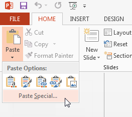
Figure 19-11: Select Paste Special from the Home tab in PowerPoint.

The Paste Special dialog box appears (see Figure 19-12).

Figure 19-12: Be sure to select Paste Link and set the link as an Excel Chart Object.

5. Select the Paste Link radio button and choose Microsoft Excel Chart Object from the list of document types.

6. Click OK to apply the link.

Your chart on your PowerPoint presentation now links back to your Excel worksheet (see Figure 19-13).

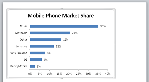
Figure 19-13: Your Excel chart is now linked into your new PowerPoint presentation.

If you’re copying multiple charts, select the range of cells that contains the charts and press Ctrl+C to copy. This way, you’re copying everything in that range of cells — charts and all.

Manually updating links to capture updates

The nifty thing about dynamic links is that they can be updated, enabling you to capture any new data in your Excel worksheets without re-creating the links. To see how this works, follow these steps:

1. Go back to your Excel file (from the example in the previous section) and change the values for Samsung and Nokia, as shown in Figure 19-14.

Note the chart has changed.

2. Return to PowerPoint, right-click the chart link in your presentation and choose Update Link, as demonstrated in Figure 19-15.

You see that your linked chart automatically captures the changes.

3. Save and close both your Excel file and your PowerPoint presentation and then open only your newly created PowerPoint presentation.

Now you see the message shown in Figure 19-16. Clicking the Update Links button updates all links in the PowerPoint presentation. Each time you open any PowerPoint presentation with links, it asks you whether you want to update the links.

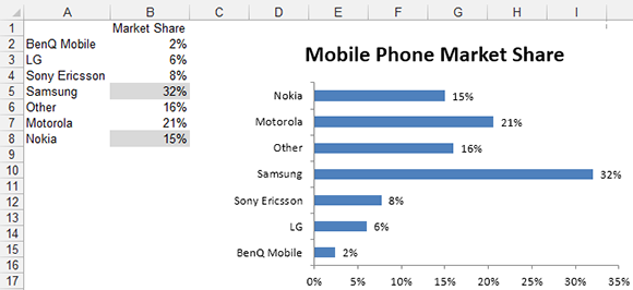
Figure 19-14: With a linked chart, you can make changes to the raw data without worrying about re-exporting the data into PowerPoint.

Figure 19-15: You can manually update links.

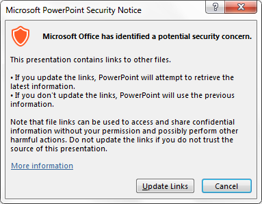
Figure 19-16: PowerPoint, by default, asks if you want to update all links in the presentation.

Automatically updating links

Having PowerPoint ask you whether you want to update the links each and every time you open your presentation quickly gets annoying. You can avoid this message by specifying that PowerPoint automatically updates your dynamic links upon opening the presentation file. Here’s how:

1. In PowerPoint, click the File tab to get to the Backstage View.

2. In the Info Pane, go to the lower-right corner of the screen and select Edit Links to Files, as shown in Figure 19-17.

The Links dialog box opens (see Figure 19-18).

3. Click each of your links and select the Automatic radio button.

Figure 19-17: Open the dialog box to manage your links.

Figure 19-18: Setting the selected links to update automatically.

When your links are set to update automatically, PowerPoint automatically synchronizes with your Excel worksheet file and ensures that all your updates are displayed.

To select multiple links in the Links dialog box, press the Ctrl key on your keyboard while you select your links.

Distributing Your Dashboards via a PDF

Starting with Excel 2010, Microsoft has made it possible to convert your Excel worksheets to a PDF document. A PDF is the standard document-sharing format developed by Adobe.

Although it may not seem intuitive to distribute your dashboards with PDF files, some distinct advantages make PDF an attractive distribution tool.

→ There are many advantages to publishing a Balanced Scorecard in PDF.

→ Distributing your reports and dashboards as a PDF file allows you to share your final product without sharing all the formulas and back-end plumbing that comes with the workbook.

→ Dashboards display in PDF files with full fidelity, meaning they display consistently on any computer and screen resolution.

→ PDF files can be used to produce high-quality prints.

→ Anyone using the free Adobe Reader can post comments and sticky notes on the distributed PDF files.

→ Unlike Excel Security, the security in a PDF is generally better, allowing for multiple levels of security, including public-key encryption and certificates.

To convert your workbook to a PDF, follow these simple steps:

1. Click the File tab and then choose the Export command.

2. In the Export pane, select Create PDF/XPS Document (see Figure 19-19).

3. The Publish as PDF or XPS dialog box opens. Click the Options button, as demonstrated in Figure 19-20.

4. In the Options dialog box (illustrated in Figure 19-21), you can specify what you want to print. You have the option of printing the entire workbook, specific pages, or a range that you’ve selected.

5. Click OK to confirm your selections.

6. Click Save.

Figure 19-19: In Excel 2013, you can natively save as PDF.

Figure 19-20: Select a location for your PDF; then click the Options button.

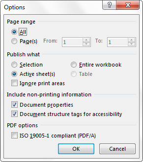
Figure 19-21: Excel allows you to define what gets sent to PDF.

Distributing Your Dashboards to SkyDrive

SkyDrive is Microsoft’s answer to Google Spreadsheets. You can think of it as a Microsoft Office platform in the cloud, allowing you to save, view, and edit your Office documents on the web.

When you publish your Excel dashboards or reports to SkyDrive, you can

→ View and edit your workbooks from any browser, even if the computer you’re using doesn’t have Excel installed.

→ Provide a platform where two or more people can collaborate on and edit the same Excel file at the same time.

→ Share only specific sheets from your workbook by hiding sheets you don’t want the public to see. When a sheet in a published workbook is hidden, the browser doesn’t even recognize its existence, so there is no way for the sheet to be unhidden or hacked into.

→ Offer up web-based interactive reports and dashboards that can be sorted and filtered.

To publish a workbook to SkyDrive, follow these steps:

1. Click the File tab on the Ribbon, click the Save As command, and choose SkyDrive, as demonstrated in Figure 19-22.

The SkyDrive pane allows you to sign in to your SkyDrive account.

If you don’t have a SkyDrive account, you can sign up for one using the Sign Up link.

Figure 19-22: Go to the SkyDrive pane.

2. Sign in to your SkyDrive account.

After signing in, the Save As dialog box in Figure 19-23 appears.

3. Click Browser View Options to select which components of your workbook will be viewable to the public.

Figure 19-23: Click Browser View Options.

The Browser View Options dialog box allows you to control what the public is able to see and manipulate in your workbook.

4. Click the Show tab (illustrated in Figure 19-24).

Here, you can check and uncheck the Sheets and other Excel objects. Removing the check next to any sheet or object prevents it from being viewable through the browser. Again, this is a fantastic way to share your dashboard interfaces without exposing the back-end calculations and data model.

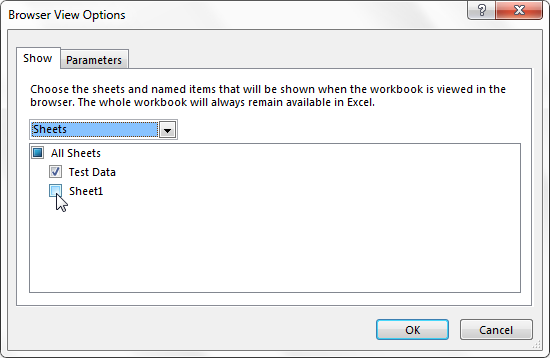
Figure 19-24: You have full control over which sheets and objects are available to the public when publishing to the web.

5. After you confirm your browser view options, save the file into your Documents folder.

At this point, you can sign in to Live.com and navigate to your SkyDrive documents to see your newly published file.

There are several ways to share your newly published workbook:

→ Copy the web link from the browser address bar and e-mail that to your cohorts.

→ Click the File tab in the web version of your file, choose Share (as shown in Figure 19-25), and then click the Share with People command to send an e-mail to anyone you specify.

→ Use the Embed command on the same Share pane to generate HTML code to embed your workbook into a web page or blog.

Figure 19-25: Sharing options in an Excel web document.

Limitations when publishing to the web

It’s important to understand that workbooks that run on the web are running in an Excel Web App that is quite different from the Excel client application you have on your PC. The Excel Web App has limitations on the features it can render in the web browser. Some limitations exist because of security issues, whereas others exist simply because Microsoft hasn’t had time to evolve the Excel Web App to include the broad set of features that come with standard Excel.

In any case, the Excel Web App has some limitations:

→ Data Validation doesn’t work on the web. This feature is simply ignored when you publish your workbook to the web.

→ No form of VBA, including macros, will run in the Excel Web App. Your VBA procedures simply will not transfer with the workbook.

→ Worksheet protection will not work on the web. Instead, you will need to plan for and use the Browser View Options demonstrated earlier in Figure 19-23.

→ Links to external workbooks will no longer work after publishing to the web.

→ You can use any pivot tables with full fidelity on the web, but you cannot create any new pivot tables while your workbook is on the web. You will need to create pivot tables in the Excel client on your PC before publishing on the web.