
Chapter 14
The z-Transform for Discrete-Time Signals
In This Chapter
![]() Traveling to the z-domain with the two-sided z-transform
Traveling to the z-domain with the two-sided z-transform
![]() Appreciating the ROC for left- and right-sided sequences
Appreciating the ROC for left- and right-sided sequences
![]() Using partial fraction expansion to return to the time domain
Using partial fraction expansion to return to the time domain
![]() Checking out z-transform theorems and pairs
Checking out z-transform theorems and pairs
![]() Visualizing how pole-zero geometry controls the frequency response
Visualizing how pole-zero geometry controls the frequency response
The z-transform (ZT) is a generalization of the discrete-time Fourier transform (DTFT) (covered in Chapter 11) for discrete-time signals, but the ZT applies to a broader class of signals than the DTFT. The ZT notation is also more user friendly than the DTFT. For example, linear constant coefficient (LCC) difference equations (see Chapter 7) can be solved by using just algebraic manipulation when the ZT is involved.
Here’s the deal: When a discrete-time signal is transformed with the ZT, it becomes a function of a complex variable; the DTFT creates a function of a real frequency variable only. The transformed signal is said to be in the z-domain.
The ZT closely parallels the Laplace transform (see Chapter 13) for continuous-time signals, and you can use the ZT to analyze signals and the impulse response of linear time-invariant (LTI) systems.
In this chapter, I introduce the two-sided ZT, which allows you to transform signals that cover the entire time axis. When computing the ZT, you immediately bump into the region of convergence (ROC), which tells you where the transform exists. This chapter also describes important ROC properties that offer insight into the nature of a signal or system.
The Two-Sided z-Transform
The two-sided or bilateral z-transform (ZT) of sequence ![]() is defined as
is defined as ![]() , where z is a complex variable. The ZT operator transforms the sequence
, where z is a complex variable. The ZT operator transforms the sequence ![]() to
to ![]() , a function of the continuous complex variable z. The relationship between a sequence and its transform is denoted as
, a function of the continuous complex variable z. The relationship between a sequence and its transform is denoted as ![]() .
.
You can establish the connection between the discrete-time Fourier transform (DTFT) and the ZT by first writing ![]() (polar form):
(polar form):

The special case of ![]() evaluates
evaluates ![]() over the unit circle —
over the unit circle — ![]() sweeps around the unit circle as
sweeps around the unit circle as ![]() varies — and is represented as
varies — and is represented as ![]() — the DTFT of
— the DTFT of ![]() (see Chapter 11). This result holds as long as the DTFT is absolutely summable (read: impulse functions not allowed).
(see Chapter 11). This result holds as long as the DTFT is absolutely summable (read: impulse functions not allowed).
The view that ![]() is
is ![]() sampled around the unit circle in the z-plane (
sampled around the unit circle in the z-plane (![]() ) shows that the DTFT has period
) shows that the DTFT has period ![]() because
because ![]() for k an integer. When
for k an integer. When ![]() ,
, ![]() ,
, ![]() ,
, ![]() , and
, and ![]() . See this solution in Figure 14-1.
. See this solution in Figure 14-1.

Figure 14-1: The unit circle in the z-plane and the relation between ![]() and
and ![]() .
.
The Region of Convergence
The ZT doesn’t converge for all sequences. When it does converge, it’s only over a region of the z-plane. The values in the z-plane for which the ZT converges are known as the region of convergence (ROC).
 Convergence of the ZT requires that
![]()
The right side of this equation shows that x[n]r-n is absolutely summable (the sum of all terms ![]() is less than infinity). This condition is consistent with the absolute summability condition for the DTFT to converge to a continuous function of
is less than infinity). This condition is consistent with the absolute summability condition for the DTFT to converge to a continuous function of ![]() (see Chapter 11).
(see Chapter 11).
Convergence depends only on ![]() , so if the series converges for
, so if the series converges for ![]() , then the ROC also contains the circle
, then the ROC also contains the circle ![]() . In this case, the general ROC is an annular region in the z-plane, as shown in Figure 14-2. If the ROC contains the unit circle, the DTFT exists because the DTFT is the ZT evaluated on the unit circle.
. In this case, the general ROC is an annular region in the z-plane, as shown in Figure 14-2. If the ROC contains the unit circle, the DTFT exists because the DTFT is the ZT evaluated on the unit circle.

Figure 14-2: The general ROC is an annulus.
The significance of the ROC
The ROC has important implications when you’re working with the ZT, especially the two-sided ZT. When the ZT produces a rational function, for instance, the roots of the denominator polynomial are related to the ROC. And for LTI systems having a rational ZT, the ROC is related to a system’s bounded-input bounded-output (BIBO) stability. The uniqueness of the ZT is also ensured by the ROC.
 Example 14-1: Consider the right-sided sequence
 ![]() . The term right-sided means that the sequence is 0 for
. The term right-sided means that the sequence is 0 for ![]() , and the nonzero values extend from n0 to infinity. The value of n0 may be positive or negative.
, and the nonzero values extend from n0 to infinity. The value of n0 may be positive or negative.
To find ![]() and the ROC, follow these steps:
and the ROC, follow these steps:
1. Reference the definition to determine the sum:
![]()
2. Find the condition for convergence by summing the infinite geometric series:
![]()
Thus, the ROC is ![]() .
.
3. To find the sum of Step 1 in closed form, use the finite geometric series sum formula (see Chapter 2):
![]()
The geometric series convergence condition corresponds with the ROC. In Examples 14-2 and 14-3, I find the ROC from the geometric series convergence condition.
Example 14-2: Consider the left-sided sequence ![]() . The term left-sided means that the sequence is 0 for
. The term left-sided means that the sequence is 0 for ![]() . To find
. To find ![]() and the ROC, write the definition and the infinite geometric series:
and the ROC, write the definition and the infinite geometric series:
![]()
If the sum looks unfamiliar in its present form, you can change variables in the sum, an action known as re-indexing the sum, by letting ![]() , then in the limits
, then in the limits ![]() ,
, ![]() , and in the sum itself
, and in the sum itself ![]() :
:

Note: Both ![]() from Example 14-1 and
from Example 14-1 and ![]() from Example 14-2 have the same ZT. The ROCs, however, are complements; the ZTs are thus distinguishable only by the ROCs being different, demonstrating that you need the ROC to return to the time domain without ambiguity — is it left-sided or right-sided? The rest of this chapter focuses exclusively on right-sided sequences, because they correspond to the most common scenarios.
from Example 14-2 have the same ZT. The ROCs, however, are complements; the ZTs are thus distinguishable only by the ROCs being different, demonstrating that you need the ROC to return to the time domain without ambiguity — is it left-sided or right-sided? The rest of this chapter focuses exclusively on right-sided sequences, because they correspond to the most common scenarios.
Plotting poles and zeros
For rational functions, such as the ![]() of Examples 14-1 and 14-2, you want to plot the pole and zero locations in the z-plane as well as the ROC. A rational
of Examples 14-1 and 14-2, you want to plot the pole and zero locations in the z-plane as well as the ROC. A rational ![]() takes the form
takes the form ![]() , where
, where ![]() and
and ![]() are both polynomials in either z or
are both polynomials in either z or ![]() . The roots of
. The roots of ![]() , where
, where ![]() , are the zeros of
, are the zeros of ![]() , and the roots of
, and the roots of ![]() are the poles of
are the poles of ![]() .
.
 I recommend placing
 ![]() in positive powers of z when determining the poles and zeros. You can do this by multiplying the numerator and denominator by the largest positive power of z to eliminate any negative powers of z.
in positive powers of z when determining the poles and zeros. You can do this by multiplying the numerator and denominator by the largest positive power of z to eliminate any negative powers of z.
Check out the pole-zero plot of ![]() , including the ROC, for
, including the ROC, for ![]() and
and ![]() in Figure 14-3.
in Figure 14-3.
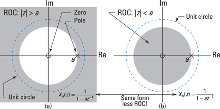
Figure 14-3: The pole-zero plot and ROC of ![]() (a) and
(a) and ![]() (b), of Examples 14-1 and 14-2.
(b), of Examples 14-1 and 14-2.
The ROC and stability for LTI systems
An LTI system is BIBO stable if the impulse response ![]() is absolutely summable, which means that the sum of all terms |h[n]| is less than infinity (see Chapter 6). To relate this to the ROC, consider the corresponding ZT
is absolutely summable, which means that the sum of all terms |h[n]| is less than infinity (see Chapter 6). To relate this to the ROC, consider the corresponding ZT ![]() , also known as the system function. You can find out whether the ROC of H(z) includes the unit circle by setting
, also known as the system function. You can find out whether the ROC of H(z) includes the unit circle by setting ![]() and then checking for absolute summability:
and then checking for absolute summability:
![]()
Here, you can conclude that, yes, the ROC of a BIBO stable system must include the unit circle.
Carrying the analysis a bit further, the poles of ![]() must sit outside the ROC because the poles of
must sit outside the ROC because the poles of ![]() sit at singularities, points where
sit at singularities, points where ![]() is unbounded. For right-sided sequences, the ROC is the exterior of a circle with a radius corresponding to the largest pole radius of
is unbounded. For right-sided sequences, the ROC is the exterior of a circle with a radius corresponding to the largest pole radius of ![]() . This is the case in Example 14-1, where
. This is the case in Example 14-1, where ![]() has a pole at
has a pole at ![]() .
.
An LTI system with impulse response ![]() and system function
and system function ![]() is BIBO stable if the ROC contains the unit circle. The system function is the ZT version of frequency response
is BIBO stable if the ROC contains the unit circle. The system function is the ZT version of frequency response ![]() .
.
For the special case of a causal system, in which ![]() for
for ![]() , the poles of
, the poles of ![]() must lie inside the unit circle because right-sided sequences, where causal sequences are a special case, have an ROC that’s the exterior of the largest pole radius of
must lie inside the unit circle because right-sided sequences, where causal sequences are a special case, have an ROC that’s the exterior of the largest pole radius of ![]() . In short, poles inside the unit circle ensure stability of causal discrete-time LTI systems.
. In short, poles inside the unit circle ensure stability of causal discrete-time LTI systems.
Example 14-3: To find ![]() given
given ![]() , use the transform pair developed in Example 14-1 with a = 1/3 and 1/2 in the first and second terms, respectively, and make use of linearity:
, use the transform pair developed in Example 14-1 with a = 1/3 and 1/2 in the first and second terms, respectively, and make use of linearity:
![]()
The ROC is the intersection of the two ROCs unless a pole-zero cancellation occurs. So, tentatively, the ROC is ![]() . When placed over a common denominator,
. When placed over a common denominator, ![]() is
is

The system pole-zero plot and ROC are shown in Figure 14-4.
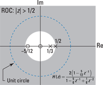
Figure 14-4: Pole-zero plot of a two-pole causal and stable system.
Finite length sequences
If ![]() has finite length (finite impulse response [FIR] in this case), then
has finite length (finite impulse response [FIR] in this case), then ![]() will converge everywhere as long as
will converge everywhere as long as ![]() is finite for all nonzero values. If
is finite for all nonzero values. If ![]() is nonzero only on
is nonzero only on ![]() , then the ZT of
, then the ZT of ![]() is simply
is simply ![]() . Here, the ROC is the entire z-plane, excluding perhaps
. Here, the ROC is the entire z-plane, excluding perhaps ![]() and/or
and/or ![]() .
.
If ![]() contains negative powers of z, then the ROC must exclude
contains negative powers of z, then the ROC must exclude ![]() (ROC:
(ROC: ![]() ) to avoid the
) to avoid the ![]() singularity. Similarly, if
singularity. Similarly, if ![]() contains positive powers of z, then the ROC must exclude
contains positive powers of z, then the ROC must exclude ![]() (ROC:
(ROC: ![]() ) to remain bounded.
) to remain bounded.
Example 14-4: Find the ZT of the finite length sequence ![]() . Note that this sequence is a rectangular window with exponential weighting
. Note that this sequence is a rectangular window with exponential weighting ![]() . Use the definition of the ZT and the finite geometric series sum formula:
. Use the definition of the ZT and the finite geometric series sum formula:
![]()
Because ![]() includes only negative powers of z, ROC:
includes only negative powers of z, ROC: ![]() . What about the poles and zeros? The denominator (poles) is clear, but you may be stuck on the numerator (zeros). The roots of
. What about the poles and zeros? The denominator (poles) is clear, but you may be stuck on the numerator (zeros). The roots of ![]() are given by
are given by ![]() ,
, ![]() (see Chapter 2 for details on the N roots of unity). The pole at
(see Chapter 2 for details on the N roots of unity). The pole at ![]() cancels the zero at
cancels the zero at ![]() . Putting it all together, you get the following:
. Putting it all together, you get the following:
![]()
This equation shows ![]() zeros equally spaced around a circle of radius a, excluding
zeros equally spaced around a circle of radius a, excluding ![]() and
and ![]() poles at
poles at ![]() . The pole-zero plot is shown in Figure 14-5 for
. The pole-zero plot is shown in Figure 14-5 for ![]() .
.
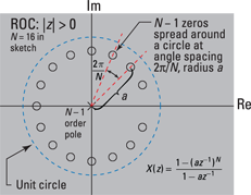
Figure 14-5: Pole-zero plot for an exponentially weighted window having length ![]() .
.
You may have noticed that the number of poles and zeros plotted is always equal to each other. This is a property of X(z) when it’s a ratio of polynomials in z or z-1. Figure 14-5 shows N – 1 poles at z = 0 and N – 1 zeros spread around a circle of radius a.
In some instances, a pole or zero may be at infinity! Consider the one-zero system (z – a). As ![]() ,
, ![]() , which is the behavior of a pole at infinity. Likewise, consider the one-pole system 1/(z – a). As
, which is the behavior of a pole at infinity. Likewise, consider the one-pole system 1/(z – a). As ![]() ,
, ![]() , which is the behavior of a zero at infinity. The next example investigates a pole at infinity following sequence shifting.
, which is the behavior of a zero at infinity. The next example investigates a pole at infinity following sequence shifting.
Example 14-5: Consider ![]() . To find
. To find ![]() , the ROC, and the poles and zeros, follow this process:
, the ROC, and the poles and zeros, follow this process:
1. Apply the definition of the ZT:
![]()
2. From ![]() , find that the zeros are
, find that the zeros are ![]() , the two poles are at
, the two poles are at ![]() , and ROC is
, and ROC is ![]() .
.
3. Generate the pole-zero plot in Figure 14-6 by using PyLab and the custom function ssd.zplane(b,a,radius=2).
Then check this on your own, using the available ssd.py Python code module.
In [17]: ssd.zplane([1,-3/2.,-1],[1],2.25)

Figure 14-6: A pole-zero plot generated by using zplane([1,-3/2.,-1],[1],2.25).
If you shift ![]() to the left one sample (let
to the left one sample (let ![]() ),
), ![]() , then the ZT becomes
, then the ZT becomes
![]()
which still has zeros at 2 and –1/2. Now the poles are at zero and infinity. You need the pole at infinity to equalize the pole-zero count and account for the fact that ![]() as
as ![]() , which is the behavior of a pole at infinity. Shifting
, which is the behavior of a pole at infinity. Shifting ![]() to the right one sample (let
to the right one sample (let ![]() ) introduces a zero at infinity; the ZT goes to zero as
) introduces a zero at infinity; the ZT goes to zero as ![]() .
.
Returning to the Time Domain
After working in the z-domain, you need to get your signal back to the time domain to work with it as a true signal once again, following some z-domain operations, such as filtering. The quick way back is through the inverse z-transform.
Formally, the inverse z-transform requires contour integration, a function of a complex variable. With a contour integral, you integrate on a closed curve in the z-plane instead of using an ordinary integral along a line. Note that I said formally. The most practical way to return from the z-domain is to form a partial fraction expansion (PFE) (see Chapter 2) and then apply the inverse z-transform to each term of the expansion by using a table of z-transform pairs.
If you can’t directly find ![]() from a list of transform pairs, such as you can find in Figure 14-8, then you can use PFE to decompose X(z) into a sum of terms that each have an inverse transform readily available. In this book, assume that
from a list of transform pairs, such as you can find in Figure 14-8, then you can use PFE to decompose X(z) into a sum of terms that each have an inverse transform readily available. In this book, assume that ![]() is expressed in negative powers of z. Start here:
is expressed in negative powers of z. Start here:
![]()
Ensure that ![]() is proper rational, or
is proper rational, or ![]() . If it isn’t, you need to use long division to reduce the order of the denominator. Example 14-6 demonstrates the long division process for polynomials written in terms of negative powers of z.
. If it isn’t, you need to use long division to reduce the order of the denominator. Example 14-6 demonstrates the long division process for polynomials written in terms of negative powers of z.
When ![]() ,
, ![]() is an improper rational function. Following long division, you end up with
is an improper rational function. Following long division, you end up with
![]()
Here, ![]() is the remainder polynomial from long division, having degree less than N.
is the remainder polynomial from long division, having degree less than N.
In this section, I run through a few PFE considerations and include examples that point out how these considerations play out in the real world.
Working with distinct poles
For the case distinct poles, if you assume that ![]() is proper rational and
is proper rational and ![]() contains no repeated roots (poles), then you can write
contains no repeated roots (poles), then you can write ![]() where the
where the ![]() ’s are the nonzero poles of
’s are the nonzero poles of ![]() and the Rk’s are the PFE coefficients.
and the Rk’s are the PFE coefficients.
 Some textbooks and references use positive powers of z for PFE, but I use negative powers of z for this technique. Don’t attempt to mix the two approaches. Using negative powers of z is the most common approach, and it fits the very nature of the signals being transformed. Signals are most often delayed in time, which corresponds to a negative power of z in the z-domain.
For the case of negative powers of z, the PFE coefficients are given by the residue formula:
![]()
If you need to perform long division, be sure to augment your final solution with the long division quotient terms ![]() .
.
Managing twin poles
When the pole ![]() for
for ![]() is repeated once (a multiplicity of two), you augment the expansion form as follows:
is repeated once (a multiplicity of two), you augment the expansion form as follows:
![]()
For the distinct poles, you can find the coefficients ![]() by using the residue formula from the previous section. For the
by using the residue formula from the previous section. For the ![]() coefficient, use a modified version of the residue formula:
coefficient, use a modified version of the residue formula:
![]()
Find ![]() by substitution. (This step is covered in Example 14-7.)
by substitution. (This step is covered in Example 14-7.)
Performing inversion
After you complete the PFE, move on to using the inverse transform of the form ![]() ,
, ![]() , and
, and ![]() to get the signal back to the time domain, one by one. Unless stated otherwise, assume that the ROC is the exterior of a circle whose radius corresponds to the largest pole radius of X(z). This assumption makes the corresponding time-domain signals right-sided.
to get the signal back to the time domain, one by one. Unless stated otherwise, assume that the ROC is the exterior of a circle whose radius corresponds to the largest pole radius of X(z). This assumption makes the corresponding time-domain signals right-sided.
Here’s the table lookup for each of the three transform types:

Using the table-lookup approach
This section contains two inverse z-transform (IZT) examples that describe how to complete PFE with the table-lookup approach. The first example requires long division but has only distinct poles; the second doesn’t require long division but has one pole repeated. In both examples, you follow these steps:
1. Find out whether X(z) is a proper rational function; if not, perform long division to make it so.
2. Find the roots of the denominator polynomial and make note of any repeated roots.
3. Write the general PFE of X(z) in terms of undetermined coefficients.
4. Solve for the coefficients by using a combination of the residue formula and substitution techniques as needed.
5. Apply the IZT to the individual PFE terms by using table lookup.
6. Check your solution by using a computer tool, such as Python.
Example 14-6: Find ![]() given the following:
given the following:
![]()
Here’s the process for returning this signal to the time domain:
1. Because the numerator and denominator are both second degree, reduce the numerator order to one or less by using long division.
In this case, you want to reduce the numerator to order zero:

The numbers are deceptively simple in this example, so work carefully.
2. Factor the denominator polynomial to find the roots.
Breathe easy, it’s already done for you in this example, but you could have started with 1 – (1/4)z–1 – (1/8)z–2. Notice that the roots, 1/2 and –1/4 are distinct.
3. Using the results of long division and the roots identified in Step 2, write out the general PFE so you can see the coefficients you need to find.

4. Solve for ![]() and
and ![]() coefficients, using the residue formula:
coefficients, using the residue formula:

5. With the PFE coefficients and long division quotient in hand, apply the inverse transform to the terms of the PFE:
![]()
The ROC is the exterior of a circle of radius 1/4 so all the time-domain terms are right-sided. Carry out the inversion of each term:
![]()
6. Check your work with PyLab and the SciPy signal package function R,p,K = residuez(b,a).
The ndarray b contains the numerator coefficients, and a contains the denominator coefficients. The function returns a tuple of three ndarrays, R (the residues), p (the poles), and K (the results of long division):
In [7]: R,p,K = signal.residuez([1,2,1],[1,-.25,-.125])
In [8]: R
Out[8]: array([3., 6.])
In [9]: p
Out[9]: array([-0.25, 0.5 ])
In [10]: K
Out[10]: array([-8.])
The Python check agrees with the hand calculation!
Example 14-7: Find ![]() given the following equation:
given the following equation:
![]()
Now go through the six-step process:
1. Examine X(z); if you find it to be proper rational as M = 0 and N = 2, no long division is required.
2. Factor the denominator polynomial to find the roots.
Here, the denominator polynomial is already in factored form, and the roots are 1/2 and 1/4 with the 1/4 repeated, making this a multiplicity of two.
3. Write the general PFE with one root repeated:
![]()
4. Using the residue formula, find that the coefficient R1 is 4. Using the modified residue formula, find that the coefficient S2 is –1.
At this point, you have the following:
![]()
Use substitution to solve for S1 in the expansion by choosing a convenient value for z–1 that doesn’t place a zero in the denominator of any term. Choosing ![]() gives you the equation
gives you the equation ![]() . With all the coefficients solved for, write
. With all the coefficients solved for, write
![]()
5. Because the ROC is the exterior of a circle of radius 1/2, all the time-domain terms are right-sided; carry out the inversion of each term to get this equation:
![]()
6. Multiply out the denominator polynomial and then check your work with Python:
![]()
Load the numerator and denominator coefficients into residuez():
In [33]: R,p,K = signal.residuez([1],[1.,-1., 5/16.,-1/32.])
In [34]: R
Out[34]: array([-2.+0.j, -1.+0.j, 4.+0.j])
In [35]: p
Out[35]: array([0.25+0.j, 0.25+0.j, 0.50+0.j])
In [36]: K
Out[36]: array([0.])
Nice. Total agreement with the hand calculation.
Surveying z-Transform Properties
The ZT has many useful theorems and transform pairs. The transform theorems can be applied generally to any signal, but the transform pairs involve a specific signal and corresponding z-transform. The transform pairs in this section emphasize right-sided signals and causal systems because that’s the emphasis of this chapter. This means that the ROC is generally the exterior of a circle having finite radius.
Transform theorems
You can find some useful z-transform theorems in Figure 14-7. All these theorems are valuable, but some are used more frequently than others. For instance, the linearity theorem (Line 1) is especially popular because it allows you to break down big problems into smaller pieces. The proof follows immediately from the definition of the ZT.

Figure 14-7: Useful ZT theorems.
In the following sections, I lavish some special attention on two theorems — the delay and convolution theorems — because they apply to so many of the problems you’re likely to encounter as an electrical engineer.
Delay
One of the most widely used ZT theorems is delay (also sometimes called time shift): ![]() . Here, the ROC is the ROC of
. Here, the ROC is the ROC of ![]() , denoted
, denoted ![]() , with the possible exclusion of zero or infinity depending on both
, with the possible exclusion of zero or infinity depending on both ![]() and the sign of
and the sign of ![]() .
.
The proof follows from the definition and the substitution ![]() :
:
![]()
Convolution
The convolution theorem of sequences is fundamental when working with LTI systems. It can be shown that ![]() , where the
, where the ![]() or larger if pole-zero cancellation occurs.
or larger if pole-zero cancellation occurs.
You can develop the proof of the convolution in two steps:
1. Insert the convolution sum into the ZT and then change the sum order:
![]()
2. Change variables on the inner sum by letting ![]() .
.
The inner sum becomes H(z), and the outer sum becomes X(z):

Transform pairs
Transform pairs are the lifeblood of working with the ZT. If you need to transform a signal or inverse transform a z-domain function, start by consulting a transform pairs table. Combined with theorems, these pairs practically give you super powers. Some basic transform pairs are developed in Examples 14-1 and 14-2, earlier in this chapter.
Example 14-8: Determine the z-transform of the sequence ![]() . From the differentiation theorem, you know that the following must be true:
. From the differentiation theorem, you know that the following must be true:

The transform pair developed is
![]()
Working with the delay theorem and linearity makes this pair into Line 5 of Figure 14-8.
Find a short table of z-transform pairs in Figure 14-8, which emphasizes right-sided sequences because that’s the focus of this chapter.
If you notice the absence of the step function, u[n], all you need to do is let a = 1 in Line 3 of Figure 14-8, and you have that pair, too!

Figure 14-8: Common ZT pairs.
Leveraging the System Function
The system function H(z) for LTI discrete-time systems, like its counterpart for continuous-time signals H(s) (see Chapter 13), plays an important role in the design and analysis of systems. Of special interest are LTI systems that are represented by a linear constant coefficient (LCC) difference equation.
When you couple the system function with the convolution theorem, you have the capability to model signals passing through systems entirely in the z-domain. In this section, I show you how the poles and zeros work together to shape the frequency response of a system.
The general LCC difference equation ![]() describes a causal system where the output y[n] is related to input x[n], M past inputs and N past outputs (see Chapter 7). You can find the system function by taking the z-transform of both sides of this equation and using linearity and the delay theorem, form the ratio of
describes a causal system where the output y[n] is related to input x[n], M past inputs and N past outputs (see Chapter 7). You can find the system function by taking the z-transform of both sides of this equation and using linearity and the delay theorem, form the ratio of ![]() to get
to get
![]()
This works as a result of the convolution theorem (see Figure 14-7), ![]() or
or ![]() .
.

 After you solve for
 ![]() , you can go almost anywhere:
, you can go almost anywhere:
![]()
![]() gives you the impulse response,
gives you the impulse response, ![]() .
.
![]()
![]() reveals the step response.
reveals the step response.
![]()
![]() provides the output
provides the output ![]() in response to input
in response to input ![]() .
.
Applying the convolution theorem
The convolution theorem gives you some powerful analysis capabilities. When you write Y(z) = X(z)H(z), the door opens to the time-domain, z-domain, and even frequency-domain results for the input, output, and the system itself. You can find Y(z), y[n] (via the inverse z-transform), and ![]() . You can also find X(z) if you’re given Y(z) first as well as H(z), because X(z) = Y(z)/H(z).
. You can also find X(z) if you’re given Y(z) first as well as H(z), because X(z) = Y(z)/H(z).
In some cases, you may have the time-domain quantities y[n] and/or h[n] instead, but getting to the z-domain is no problem because ![]() and
and ![]() . Or, given X(z) and Y(z), you can discover the system function H(z) with a starting point of the time-domain quantities.
. Or, given X(z) and Y(z), you can discover the system function H(z) with a starting point of the time-domain quantities.
Example 14-9: You’re given the system input ![]() and LTI system function
and LTI system function
![]()
To find the system output ![]() , the most direct approach is to find
, the most direct approach is to find ![]() and then calculate the inverse transform to get
and then calculate the inverse transform to get ![]() . Using transform pair Line 3 from Figure 14-8, you can write
. Using transform pair Line 3 from Figure 14-8, you can write
![]()
Solve for the coefficients:

By calculating the inverse z-transform term by term, you get this equation: ![]() .
.
Check your results in PyLab or Maxima to verify that your hand calculations are correct.
Finding the frequency response with pole-zero geometry
The poles and zeros of a system function control the frequency response ![]() . Consider the following development:
. Consider the following development:

where pk and zk are the poles and zeros of ![]() and
and ![]() , and
, and ![]() are the frequency response contributions of each pole and zero. The vectors
are the frequency response contributions of each pole and zero. The vectors ![]() point from the zero and pole locations to the point
point from the zero and pole locations to the point ![]() on the unit circle. This gives you a connection between the pole-zero geometry and the frequency response. In particular, the ratio of vector magnitudes,
on the unit circle. This gives you a connection between the pole-zero geometry and the frequency response. In particular, the ratio of vector magnitudes, ![]() , is the magnitude response. The phase response is
, is the magnitude response. The phase response is ![]()
![]() .
.
Two custom software apps, PZ_Geom and PZ_Tool, at www.dummies.com/extras/signalsandsystems can help you further explore the relationship between frequency response and pole-zero location.
![]()
PZ_Geom app: You can load a predefined system or filter or load custom coefficients and then see the pole-zero geometry with the geometry lines to represent the vectors ![]() and
and ![]() that change as you drag
that change as you drag ![]() with the mouse. A marker on the magnitude and frequency response follows along in adjacent plots.
with the mouse. A marker on the magnitude and frequency response follows along in adjacent plots.
![]()
PZ_Tool app: You can place and then drag poles and zeros arbitrarily over the z-plane to see the magnitude and phase response change interactively as poles and zeros are moved.
Example 14-10: Consider the simple first-order system:
![]()
This system contains single numerator and denominator vectors, so the geometry is rather simple: ![]() . The software app
. The software app PZ_Geom allows you to see magnitude and angle of the vectors change as ![]() is changed by dragging the mouse. The result is that you're able to explore the relationship between frequency response and pole-zero location. A screen shot of
is changed by dragging the mouse. The result is that you're able to explore the relationship between frequency response and pole-zero location. A screen shot of PZ_geom is shown Figure 14-9.
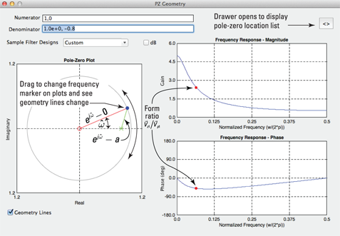
Figure 14-9: The pole-zero geometry app allows you to drag the ![]() point on the unit circle.
point on the unit circle.