
Chapter 9
Simulation
So far we have provided a functional description of the LTE (Long Term Evolution) PHY (Physical Layer) standard and its implementation in MATLAB®. To verify whether this functional model will meet the requirements of the standardization process, we need to perform large-scale simulations. Like many other standards, the LTE standard has a mode-based specification. This means we need to perform a series of simulations in order to ensure that all possible combinations of modes, including modulation, coding, and MIMO (Multiple Input Multiple Output) modes, are exercised. The combined effects of using large simulation data sets and the computationally complex nature of the LTE standard will inevitably result in a familiar challenge: exceedingly long simulation times and the necessity to accelerate the speed of simulations.
The simulations can be performed on a software model or on a physical hardware prototype. Most designers find it useful to first run a computer model of the standard to verify various technical aspects related to the system performance before proceeding to a hardware prototype. When talking about accelerating the execution of a software model, it is natural to start with a baseline or initial version. The optimizations that lead to acceleration of the simulation speed of the baseline algorithm may or may not alter the functional accuracy of the model. To be true to a standard implementation, in this book we only highlight optimizations that preserve the numerical accuracy of the baseline algorithms. As such, optimizations examined here highlight various ways of implementing the same functionality more efficiently. In this chapter we discuss in detail many optimizations in MATLAB and Simulink that result in substantial acceleration of the simulation speed.
9.1 Speeding Up Simulations in MATLAB
When we model and simulate a communications system, our focus and priorities may be different at different stages of the workflow. In the early stages of development, we might focus on accuracy in expressing the mathematical model. At this stage we want to use visualization and debugging features of the MATLAB environment to ensure that the sequence of operations in the MATLAB function and scripts is correct. This stage of functional verification is sometimes referred to as unit testing and involves testing a limited set of data for which the correct response is known. Unit testing helps make sure that the mathematical model correctly implements the design. After satisfying the unit-testing requirements, most designers execute the same simulation model with a large amount of data within a simulation loop. Identifying the bottlenecks of design in large-scale testing helps us focus on the portions in which optimization efforts provide the most return. We can optimize the baseline model and resolve design bottlenecks in one of two ways (see Figure 9.1):
Figure 9.1 Simulation acceleration methods in MATLAB

- MATLAB code optimization: Involves changing the MATLAB program code for a more efficient implementation. This includes steps that: (i) ensure constant parameters are only computed once during initializations, (ii) reduce parameter validation overhead, (iii) use variables that are preallocated in order to avoid overhead of dynamic memory allocations, and (iv) use more efficient algorithms implemented with System objects.
- Use of acceleration features: Involves applying such techniques as: (i) converting MATLAB code to a compiled C code, (ii) exploiting multiple cores or clusters for parallel processing, or (iii) using MATLAB features that are optimized for Graphics Processing Unit (GPU) processing.
9.2 Workflow
In this chapter, we start with a baseline MATLAB program. Following a series of code optimizations, we then successively accelerate the speed of simulation. At each step, the algorithm generates the same numerical outputs. The only difference between steps is the introduction of a more efficient programming technique.
Both numerical and timing results provided throughout the book depend on the platform where MATLAB is installed, and the type of operating system, C/C++ compiler or GPU that is used. Results in this book for non-GPU experiments are obtained by running MATLAB on a laptop computer with the following specifications:
- Hardware: Intel Dual-Core i7-2620M CPU @ 2.70 GHz with 8 GB of RAM
- Operating system: 64-bit Windows 7 Enterprise (Service Pack 1)
- C/C++ compiler: Microsoft Visual Studio 2010 with Microsoft Windows SDK v7.1.
The GPU experiments use NVIDIA Tesla GPU Accelerators installed on a desktop computer with an Intel Quad-core i7 CPU with 12 GB of RAM and the same operating system and C/C++ compiler as mentioned above.
9.3 Case Study: LTE PDCCH Processing
We use a simplified version of the signal processing applied to the Physical Downlink Control Channel (PDCCH) of the LTE standard in this chapter as a case study. We have already showcased this algorithm in Chapter 7. As Figure 9.2 illustrates, processing the PDCCH signal in the transmitter side involves the following operations: Cyclic Redundancy Check (CRC) generation, tail-biting convolutional encoding, rate matching, scrambling, Quadrature Phase Shift Keying (QPSK) modulation, and transmit-diversity MIMO encoding. Channel modeling consists of a combination of a two-by-two MIMO channel and an Additive White Gaussian Noise (AWGN) channel. We perform the inverse operations at the receiver, including transmit-diversity MIMO combination, QPSK demodulation, descrambling, rate dematching, Vitetbi decoding, and CRC detection. To reduce the complexity of the algorithm, in this section we will update it with two modifications: (i) omission of the frequency-domain transformations involving Orthogonal Frequency Division Multiplexing (OFDM) resource-grid formation and signal generation; and (ii) use of hard-decision demodulation at the receiver.
Figure 9.2 A simplified PDCCH signal processing chain

9.4 Baseline Algorithm
The following baseline function shows the first implementation of the PDCCH processing chain. The sequence of operations characterizing the PDCCH algorithm already described is implemented with a series of functions. Some of the functions, such as convenc and vitdec, and objects, such as modem.pskmod and crc.generator, are available in the Communications System Toolbox. Others, such as TransmitDiversityEncoder1 and MIMOFadingChan, are user-defined and are composed using a combination of basic MATLAB functions and constructs.
function [ber, bits]=zPDCCH_v1(EbNo, maxNumErrs, maxNumBits)
%% Constants
FRM=2048;
M=4; k=log2(M); codeRate=1/3;
snr = EbNo + 10*log10(k) + 10*log10(codeRate);
trellis=poly2trellis(7, [133 171 165]);
L=FRM+24;C=6; Index=[L+1:(3*L/2) (L/2+1):L];
%% Initializations
persistent Modulator Demodulator  CRCgen CRCdet
if isempty(Modulator)
    Modulator=modem.pskmod('M', 4, 'PhaseOffset', pi/4, 'SymbolOrder', 'Gray',
'InputType', 'Bit');
    Demodulator= modem.pskdemod('M', 4, 'PhaseOffset', pi/4, 'SymbolOrder', 'Gray',
'OutputType', 'Bit');
    CRCgen = crc.generator([1 1 zeros(1, 16) 1 1 0 0 0 1 1]);
    CRCdet = crc.detector   ([1 1 zeros(1, 16) 1 1 0 0 0 1 1]);
end
%% Processing loop modeling transmitter, channel model and receiver
numErrs = 0; numBits = 0; nS=0;
while ((numErrs < maxNumErrs) && (numBits < maxNumBits))
    % Transmitter
    u               = randi([0 1], FRM,1);
    u1             = generate(CRCgen,u);
    u2             = u1((end-C+1):end);
    [˜, state] = convenc(u2,trellis);
    u3             = convenc(u1,trellis,state);
    u31           = fcn_RateMatcher(u3, L, codeRate);
    u32           = fcn_Scrambler(u31, nS);
    u4             = modulate(Modulator, u32);
    u5             = TransmitDiversityEncoder1(u4);
   % Channel model
    [u6, h6]    = MIMOFadingChan(u5);
    u7             = awgn(u6,snr);
   % Receiver
    u8             =  TransmitDiversityCombiner1(u7, h6);
    u9             = demodulate(Demodulator,u8);
    u91           = fcn_Descrambler(u9, nS);
    u92           = fcn_RateDematcher(u91, L);
    uA             = [u999;u999];
    uB             = vitdec(uA ,trellis,34,'trunc','hard');
    uC             = uB(Index);
    y                = detect(CRCdet, uC );
    numErrs      = numErrs + sum(y˜=u);
    numBits      = numBits + FRM;
    nS              = nS + 2; nS = mod(nS, 20);
end
%% Clean up & collect results
ber = numErrs/numBits;
bits=numBits;
Let us start by running this baseline algorithm to establish a benchmark for performance. The following MATLAB script (zPDCCH_v1_test) executes this algorithm within a for loop. In each iteration, the script calls the baseline algorithm with given Signal-to-Noise Ratio (SNR) values and computes the Bit Error Rate (BER). It also uses a combination of MATLAB tic and toc functions to measure the time needed to complete the loop iterations.
MaxSNR=8;
MaxNumBits=1e5;
fprintf(1,'
Version 1: Baseline algorithm

');
tic;
for snr=1:MaxSNR
    fprintf(1,'Iteration number %d
',snr);
    ber= zPDCCH_v1 (snr, MaxNumBits, MaxNumBits);
end
time_1=toc;
fprintf(1,'Version 1: Time to complete %d iterations = %6.4f (sec)
',
MaxSNR, time_1);
When we execute the MATLAB script, messages regarding the version of the algorithm, the iteration that is being executed, and the final tally of elapsed time will print in the command prompt. The results are shown in Figure 9.3. In this case, processing of 1 million bits in each of the eight iterations of the baseline algorithm takes about 411.30 seconds to complete.
Figure 9.3 Baseline algorithm: time taken to execute eight iterations

We use this measure as a yard stick and try to improve the performance using the code optimizations discussed later. Before proceeding to any code optimization, it is important to identify the code bottlenecks. These are the portions of the algorithm that contribute most to its computational complexity and take up the most processing time. We will now use some MATLAB tools to identify the bottlenecks in our algorithm.
9.5 MATLAB Code Profiling
MATLAB provides a variety of tools to help assess and optimize the performance of code. MATLAB Profiler shows where code is spending its time. It can be applied to the baseline algorithm by performing the following three commands:
profile on;
ber= zPDCCH_v1 (snr, MaxNumBits, MaxNumBits);
profile viewer;
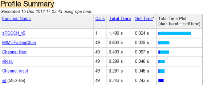
Calling the profile viewer command brings up the MATLAB Profiler report as illustrated in Figure 9.4. MATLAB Profiler provides a summary report of statistics on the overall execution of a code, including a list of all functions called, the number of times each function was called, and the total time spent in each function. It can also provide timing information about each function, such as information on the lines of code that use the most processing time.
Figure 9.4 Profile summary report for the baseline algorithm

Once bottlenecks have been identified, we can focus on improving the performance of these particular sections. For example, in this profile summary the function TransmitDiversityCombiner takes 4.385 seconds of the 7.262 seconds it takes to run the entire function. That qualifies the TransmitDiversityCombiner function as one of the bottlenecks of our baseline algorithm.
function y = TransmitDiversityCombiner1(in, chEst)
%#codegen
% Alamouti Transmit Diversity Combiner
% Scale
in = sqrt(2) * in;
% STBC Alamouti
y =  Alamouti_Decoder1(in, chEst);
% Space-Frequency to Space-Time transformation
y(2:2:end) = -conj(y(2:2:end));
When we drill down through the function hyperlink in the profile summary report, we can find out exactly which lines of the TransmitDiversityCombiner1 function take the most time. Of the three lines of code, Alamouti_Decoder1 can be easily identified as the processing bottleneck. The following Alamouti_Decoder1 function shows the first implementation of the Alamouti combining algorithm.
function s = Alamouti_Decoder1(u,H)
%#codegen
% STBC_DEC STBC Combiner
%   Outputs the recovered symbol vector
LEN=size(u,1);
Nr=size(u,2);
BlkSize=2;
NoBlks=LEN/BlkSize;
% Initialize outputs
h=complex(zeros(1,2));
s=complex(zeros(LEN,1));
% Alamouti code for 2 Tx
indexU=(1:BlkSize);
for m=1:NoBlks
    t_hat=complex(zeros(BlkSize,1));
    h_norm=0.0;
    for n=1:Nr
        h(:)=H(2*m-1,:,n);
        h_norm=h_norm+real(h*h');
        r=u(indexU,n);
        r(2)=conj(r(2));
        shat=[conj(h(1)), h(2); conj(h(2)), -h(1)]*r;
        t_hat=t_hat+shat;
    end
    s(indexU)=t_hat/h_norm; % Maximum-likelihood combining
    indexU=indexU+BlkSize;
end
end
By following the hyperlink to the Alamouti_Decoder1 function, we can see a more detailed line-by-line profile of execution time (Figure 9.5). This level of breakdown enables us to identify what feature of the code contributes most to its performance. In this case, the algorithm performs two nested for loops and computes every element of a vector one by one within a scalar programming routine. Vectorizing this code can lead to acceleration.
Figure 9.5 Line-by-line processing time in the Alamouti_Decoder1 function

9.6 MATLAB Code Optimizations
In this section we discuss some typical code-optimization techniques in MATLAB. These techniques include vectorizing the code, preallocating data, separating initialization from in-loop processing, and using System objects. To illustrate these techniques, we continue updating and optimizing the PDCCH processing algorithm.
9.6.1 Vectorization
Vectorization is one of the most important code-optimization techniques in MATLAB. In vectorization, we convert a code from using loops to using matrix and vector operations. Since MATLAB uses processor-optimized libraries for matrix and vector computations, we can often gain performance improvement by vectorizing our code.
The second version of the PDCCH algorithm is optimized based on vectorization. The only difference between this version of the algorithm and the baseline is the use of the TransmitDiversityCombine2 function instead of TransmitDiversityCombine1. This function is the second version of the transmit-diversity combiner function and uses the Alamouti_Decoder2 function, a vectorized version of Alamouti_Decoder1. When we examine the Alamouti_Decoder2 function, we can see that the nested double for loop is modified to a single for loop and that operations are more vectorized in the single loop. These changes are illustrated in the following function:
| MATLAB function | |
function [ber, bits]=zPDCCH_v1(…)
.
.
_____________________________
u5 = TransmitDiversityDecoder1(u4);
_____________________________
.
.
end |
function [ber, bits]=zPDCCH_v2(…)
.
.
_____________________________
u5 = TransmitDiversityDecoder2(u4);
_____________________________
.
.
end |
function y = TransmitDiversityCombiner1(in, chEst) %#codegen % Alamouti Transmit Diversity Combiner % Scale in = sqrt(2) * in; % STBC Alamouti _____________________________ y = Alamouti_Decoder1(in, chEst); _____________________________ % Space-Frequency to Space- Time transformation y(2:2:end) = -conj(y(2:2:end)); |
function y = TransmitDiversityCombiner2(in, chEst) %#codegen % Alamouti Transmit Diversity Combiner % Scale in = sqrt(2) * in; % STBC Alamouti _____________________________ y = Alamouti_Decoder2(in, chEst); _____________________________ % Space-Frequency to Space- Time transformation y(2:2:end) = -conj(y(2:2:end)); |
function s = Alamouti_Decoder1(u,H) LEN=size(u,1); Nr=size(u,2); BlkSize=2; NoBlks=LEN/BlkSize; % Initialize outputs h=complex(zeros(1,2)); s=complex(zeros(LEN,1)); % Alamouti code for 2 Tx indexU=(1:BlkSize); _____________________________ for m=1:NoBlks t_hat=complex(zeros(BlkSize,1)); h_norm=0.0; for n=1:Nr _____________________________ h(:)=H(2*m-1,:,n); h_norm=h_norm+real(h*h'); r=u(indexU,n); r(2)=conj(r(2)); shat=[conj(h(1)), h(2); conj(h(2)), -h(1)]*r; t_hat=t_hat+shat; end s(indexU)=t_hat/h_norm; % Maximum- likelihood combining indexU=indexU+BlkSize; end end |
function s = Alamouti_Decoder2(u,H) LEN=size(u,1); BlkSize=2; NoBlks=LEN/BlkSize; T=[0 1;-1 0]; % Initialize outputs s=complex(zeros(LEN,1)); % Alamouti code for 2 Tx h=complex(zeros(BlkSize,BlkSize)); _____________________________ for m=1:NoBlks _____________________________ indexU=(m-1)*BlkSize+(1:BlkSize); h(:)=H(2*m-1,:,:); h_norm=sum(h(:).*conj(h(:))); r=u(indexU,:); r(2,:)=conj(r(2,:)); H1=conj(h); H2=T*h; M=[H1(:,1),H2(:,1),H1(:,2),H2(:,2)]; s(indexU)=(M*r(:))/h_norm; % Maximum- likelihood combining end |
In order to verify whether this optimization leads to a faster execution time, we run the following MATLAB script. This script is identical to the one we used for the baseline algorithm except that it calls the second version of the PDCCH algorithm (zPDCCH_v2.m). This time, processing 1 million bits in eight iterations takes about 326.50 seconds to complete (Figure 9.6).
Figure 9.6 Second version of the algorithm: time taken to execute eight iterations

MaxSNR=8;
MaxNumBits=1e5;
fprintf(1,'
Version 1: Baseline algorithm

');
tic;
for snr=1:MaxSNR
    fprintf(1,'Iteration number %d
',snr);
    ber= zPDCCH_v2 (snr, MaxNumBits, MaxNumBits);
end
time_2=toc;
fprintf(1,'Version 1: Time to complete %d iterations = %6.4f (sec)
', MaxSNR, time_2);
The second version of the algorithm performs a single for loop with a number of iterations specified by the NoBlks variable, which relates to the first dimension of the function input. The first dimension is a rather large number: 3108 in this algorithm. Frequent iteration based on the first dimension and performance of vectorized operations on smaller-sized vectors does not take optimal advantage of vectorization.
The third version of the algorithm is designed to vectorize along the first dimension of the input function. In this version, we iterate only twice (along the second dimension) and perform vectorized operations on large vectors and matrices along the first dimension. It features better optimization based on vectorization of the code with large vectors and matrices. The only difference between this version and the second is the use of TransmitDiversityCombine3 instead of TransmitDiversityCombine2.
| MATLAB function | |
function [ber, bits]=zPDCCH_v2(…)
.
.
_____________________________
u5 = TransmitDiversityDecoder2(u4);
_____________________________
.
.
end |
function [ber, bits]=zPDCCH_v3(…)
.
.
_____________________________
u5 = TransmitDiversityDecoder3(u4);
_____________________________
.
.
end |
function y = TransmitDiversityCombiner2(in, chEst) %#codegen % Alamouti Transmit Diversity Combiner % Scale in = sqrt(2) * in; % STBC Alamouti _____________________________ y = Alamouti_Decoder2(in, chEst); _____________________________ % Space-Frequency to Space- Time transformation y(2:2:end) = -conj(y(2:2:end)); |
function y = TransmitDiversityCombiner3(in, chEst) %#codegen % Alamouti Transmit Diversity Combiner % Scale in = sqrt(2) * in; % STBC Alamouti _____________________________ y = Alamouti_Decoder3(in, chEst); _____________________________ % Space-Frequency to Space- Time transformation y(2:2:end) = -conj(y(2:2:end)); |
function s = Alamouti_Decoder2(u,H) LEN=size(u,1); BlkSize=2; function s = Alamouti_Decoder2(u,H) LEN=size(u,1); BlkSize=2; NoBlks=LEN/BlkSize; T=[0 1;-1 0]; % Initialize outputs s=complex(zeros(LEN,1)); % Alamouti code for 2 Tx h=complex(zeros(BlkSize,BlkSize)); _____________________________ for m=1:NoBlks _____________________________ indexU=(m-1)*BlkSize+(1:BlkSize); h(:)=H(2*m-1,:,:); h_norm=sum(h(:).*conj(h(:))); r=u(indexU,:); r(2,:)=conj(r(2,:)); H1=conj(h); H2=T*h; M=[H1(:,1),H2(:,1),H1(:,2),H2(:,2)]; s(indexU)=(M*r(:))/h_norm; % Maximum- likelihood combining end |
function y = Alamouti_Decoder3(u,Ch) %#codegen % STBC_DEC STBC Combiner LEN=size(u,1); BlkSize=2; NoBlks=LEN/BlkSize; Nr=size(u,2); idx1=1:BlkSize:LEN; idx2=idx1+1; % Initalize outputs s=complex(zeros(LEN,Nr)); mynorm=complex(zeros(LEN,BlkSize)); vec_u=complex(zeros(NoBlks,BlkSize)); % Alamouti code for 2 Tx H=complex(zeros(NoBlks,BlkSize)); _____________________________ for n=1:Nr _____________________________ vec_u(:,1) = u(idx1,n); vec_u(:,2) = conj(u(idx2,n)); H(:) = Ch(1:BlkSize:end,:,n); conjH = conj(H); cn1 = [conjH(:,1), H(:,2)]; s(idx1,n) = sum(cn1.*vec_u,2); mynorm(idx1,n) = sum(H.*conj(H),2); cn2 = [conjH(:,2), -H(:,1)]; s(idx2,n) = sum(cn2.*vec_u,2); end; nn=sum(mynorm,2); nn(idx2)=nn(idx1); y=sum(s,2)./nn; end |
In order to verify whether this optimization leads to a faster execution time, we run the following MATLAB script (zPDCCH_v3_test). The third version of the algorithm takes about 175.84 seconds to process 1 million bits in eight iterations, as illustrated in Figure 9.7.
Figure 9.7 Third version of the algorithm: time taken to execute eight iterations

MaxSNR=8;
MaxNumBits=1e5;
fprintf(1,'
Version 3: Better vectorized algorithm

');
tic;
for snr=1:MaxSNR
    fprintf(1,'Iteration number %d
',snr);
    ber= zPDCCH_v3 (snr, MaxNumBits, MaxNumBits);
end
time_3=toc;
fprintf(1,'Version 3: Time to complete %d iterations = %6.4f (sec)
', MaxSNR, time_3);
By profiling the third version of the algorithm (zPDCCH_v3), we identify the function TransmitDiversityEncoder1 as the next bottleneck. This function calls the first version of the Alamouti encoder function (Alamouti_Encoder1). The MATLAB profiler commands and resulting report are shown in Figure 9.8.
Figure 9.8 Profile summary report for the third version of the algorithm

profile on;
ber= zPDCCH_v3(snr, MaxNumBits, MaxNumBits);
profile viewer;
By following the hyperlink to the Alamouti_Encoder1 function in the profile report, we can see a more detailed line-by-line profile of the execution time (Figure 9.9). Note that we initialize output matrix y with an empty matrix. In iterations of the for loop, we then grow the size of matrix y by appending a 2 × 2 Alamouti matrix to its end. In successive iterations, we must allocate new memory and copy the existing matrix into the new one. We can thus identify preallocation as a feature of the code that can be improved. Next we will discuss preallocation as a MATLAB code-optimization feature.
Figure 9.9 Profiling Alamouti_Encoder1

9.6.2 Preallocation
Preallocation refers to the initialization of an array of known size at the beginning of a computation. It helps prevent dynamic resizing of an array while a code is executing, especially when using for and while loops. Since arrays require contiguous blocks of memory, repeated resizing of them often compells MATLAB to spend time looking for larger contiguous blocks and then moving the array into them. By preallocating arrays, we can avoid these unnecessary memory operations and improve overall execution time.
The fourth version of the PDCCH algorithm is optimized based on preallocation. This version uses the function TransmitDiversityEncoder2 instead of TransmitDiversityEncoder1; this function uses the second version of the transmit diversity encoder function, which in turn uses Alamouti_Encoder2, a preallocated version of Alamouti_Encoder1.
function [ber, bits]=zPDCCH_v4(EbNo, maxNumErrs, maxNumBits)
%% Constants
FRM=2048;
M=4; k=log2(M); codeRate=1/3;
snr = EbNo + 10*log10(k) + 10*log10(codeRate);
trellis=poly2trellis(7, [133 171 165]);
L=FRM+24;C=6; Index=[L+1:(3*L/2) (L/2+1):L];
%% Initializations
persistent Modulator Demodulator  CRCgen CRCdet
if isempty(Modulator)
    Modulator     = modem.pskmod('M', 4, 'PhaseOffset', pi/4, 'SymbolOrder', 'Gray',
'InputType', 'Bit');
    Demodulator = modem.pskdemod('M', 4, 'PhaseOffset', pi/4, 'SymbolOrder', 'Gray',
'OutputType', 'Bit');
    CRCgen         = crc.generator([1 1 zeros(1, 16) 1 1 0 0 0 1 1]);
    CRCdet          = crc.detector   ([1 1 zeros(1, 16) 1 1 0 0 0 1 1]);
end
%% Processing loop
numErrs = 0; numBits = 0; nS=0;
while ((numErrs < maxNumErrs) && (numBits < maxNumBits))
    % Transmitter
    u               = randi([0 1], FRM,1);                             % Generate bit payload
    u1             = generate(CRCgen,u);                           % CRC insertion
    u2             = u1((end-C+1):end);                              % Tail-biting convolutional coding
    [˜, state]  = convenc(u2,trellis);
    u3             = convenc(u1,trellis,state);
    u4             = fcn_RateMatcher(u3, L, codeRate);    % Rate matching
    u5             = fcn_Scrambler(u4, nS);                        % Scrambling
    u6             = modulate(Modulator, u5);                   % Modulation
    u7             = TransmitDiversityEncoder2(u6);          % MIMO Alamouti encoder
    % Channel
    [u8, h8]    = MIMOFadingChan(u7);                         % MIMO fading channel
    sigpower = 10*log10(real(var(u8(:))));
    u9             = awgn(u8,snr,sigpower,'dB');
    % Receiver
    uA             =  TransmitDiversityCombiner3(u9, h8); % MIMO Alamouti combiner
    uB             = demodulate(Demodulator,uA);             % Demodulation
    uC             = fcn_Descrambler(uB, nS);                     % Descrambling
    uD             = fcn_RateDematcher(uC, L);                  % Rate de-matching
    uE             = [uD;uD];                                                 % Tail-biting
    uF             = vitdec(uE ,trellis,34,'trunc','hard');        % Viterbi decoding
    uG            = uF(Index);
    y               = detect(CRCdet, uG );                              % CRC detection
    numErrs   = numErrs + sum( y˜=u );                           % Update number of bit errors
    numBits   = numBits + FRM;
    nS             = nS + 2; nS = mod(nS, 20);
end
%% Clean up & collect results
ber = numErrs/numBits;
bits=numBits;
When we examine Alamouti_Encoder2, we can see that it first initializes the output with information derived from the size of the input, then transforms the input and inserts selected samples of it into the predetermined locations of the output matrix. Also, the updated Alamouti_Encoder2 function is not only preallocated but also vectorized, whereas Alamouti_Encoder1 is a scalarized function. The main problem with Alamouti_Encoder1 is that it initializes the output to an empty matrix and then performs a for loop in which in each iteration the output matrix grows in size. These types of frequent dynamic memory allocation contribute to the degradation of performance.
| MATLAB function | |
function [ber, bits]=zPDCCH_v3(…)
.
.
_____________________________
u7 = TransmitDiversityEncoder1(u6);
_____________________________
.
.
end |
function [ber, bits]=zPDCCH_v4(…)
.
.
_____________________________
u7 = TransmitDiversityEncoder2(u6);
_____________________________
.
.
end |
function y = TransmitDiversityEncoder1(in) % Alamouti Transmit Diversity Encoder % Space-Frequency to Space- Time transformation in(2:2:end) = -conj(in(2:2:end)); % STBC Alamouti _____________________________ y = Alamouti_Encoder1(in); _____________________________ % Scale y = y/sqrt(2); |
function y = TransmitDiversityEncoder2(in) % Alamouti Transmit Diversity Encoder % Space-Frequency to Space- Time transformation in(2:2:end) = -conj(in(2:2:end)); % STBC Alamouti _____________________________ y = Alamouti_Encoder2(in); _____________________________ % Scale y = y/sqrt(2); |
function y= Alamouti_Encoder1(u) % Space-Time Block Encoder Tx=2; LEN=size(u,1); idx1=1:Tx:LEN-1; idx2=idx1+1; % Alamouti Space-Time Block Encoder % G = [ s1 s2 ] % [ -s2* s1*] y=[]; for n=1:LEN/Tx G=[ u(idx1(n)) u(idx2(n));… -conj(u(idx2(n))) conj(u(idx1(n)))]; y=[y;G]; end |
function y= Alamouti_Encoder2(u) % Space-Time Block Encoder Tx=2; LEN=size(u,1); idx1=1:Tx:LEN-1; idx2=idx1+1; % Alamouti Space-Time Block Encoder % G = [ s1 s2 ] % [ -s2* s1*] y=complex(zeros(LEN,Tx)); y(idx1,1)=u(idx1); y(idx1,2)=u(idx2); y(idx2,1)=-conj(u(idx2)); y(idx2,2)=conj(u(idx1)); |
By running the following MATLAB script, we can verify whether this optimization leads to a faster execution time. The results show that processing of 1 million bits in eight iterations takes about 82.71 seconds (Figure 9.10).
Figure 9.10 Fourth version of the algorithm: time taken to execute eight iterations

MaxSNR=8;
MaxNumBits=1e5;
fprintf(1,'
Version 4: Vectorization + Preallocation

');
tic;
for snr=1:MaxSNR
    fprintf(1,'Iteration number %d
',snr);
    ber= zPDCCH_v4 (snr, MaxNumBits, MaxNumBits);
end
time_4=toc;
fprintf(1,'Version 4: Time to complete %d iterations = %6.4f (sec)
',
MaxSNR, time_4);
This series of optimizations reveals a pattern. We started with a baseline algorithm that implemented the Alamouti encoder and combiner algorithms with the simplest MATLAB code. The baseline code can be considered the transcribed version of the mathematical formula of the algorithm, which can be obtained from any textbook describing space–time block coding. MATLAB codes based on scalar operations may not be sufficient to run the same algorithm with a faster execution time. In most cases, we need to alter the sequence of operations in order to leverage the vector-based character of the MATLAB language. This means implementing the same algorithm by vectorizing the code and preallocating data.
However, these extra optimizations lead to rewriting of the MATLAB code. We can either spend time optimizing our code or, if we have access to them, take advantage of the functionality available in various MATLAB toolboxes. MATLAB toolboxes are written in such a way as to be sensitive to simulation performance. All MATLAB toolbox functions are based on preallocation and vectorization. Furthermore, as discussed earlier, DSP and the Communications System Toolbox provide efficient algorithmic components as System objects. In the next section we will take advantage of some of the System objects in the Communications System Toolbox to obtain faster implementations of many components of this algorithm.
9.6.3 System Objects
System objects can be used to accelerate a MATLAB code, largely in the areas of signal processing and communications. System objects are MATLAB object-oriented implementations of algorithms available in MATLAB toolboxes such as the Communications System Toolbox. By using System objects, we decouple the declaration (System object creation) from the execution of an algorithm, resulting in more efficient loop-based calculations, since we can perform parameter handling and initializations only once. A System object can be created and configured outside the loop, and then the step method can be called inside it. A majority of System objects from the DSP and Communications System Toolbox are implemented as MATLAB Executables (MEXs). A MEX implementation of a code is essentially a compiled C code. This can also speed up simulation, since many algorithmic optimizations have been included in the MEX implementations of objects.
The fifth version of the PDCCH algorithm uses System objects of the Communications System Toolbox to implement the Alamouti encoder (Alamouti_EncoderS function) and the Alamouti combiner (Alamouti_CombinerS function).
function [ber, bits]=zPDCCH_v5(EbNo, maxNumErrs, maxNumBits)
%% Constants
FRM=2048;
M=4; k=log2(M); codeRate=1/3;
snr = EbNo + 10*log10(k) + 10*log10(codeRate);
trellis=poly2trellis(7, [133 171 165]);
L=FRM+24;C=6; Index=[L+1:(3*L/2) (L/2+1):L];
%% Initializations
persistent Modulator Demodulator  CRCgen CRCdet
if isempty(Modulator)
    Modulator     = modem.pskmod('M', 4, 'PhaseOffset', pi/4, 'SymbolOrder', 'Gray',
'InputType', 'Bit');
    Demodulator = modem.pskdemod('M', 4, 'PhaseOffset', pi/4, 'SymbolOrder', 'Gray',
'OutputType', 'Bit');
    CRCgen         = crc.generator([1 1 zeros(1, 16) 1 1 0 0 0 1 1]);
    CRCdet          = crc.detector   ([1 1 zeros(1, 16) 1 1 0 0 0 1 1]);
end
%% Processing loop
numErrs = 0; numBits = 0; nS=0;
while ((numErrs < maxNumErrs) && (numBits < maxNumBits))
    % Transmitter
    u               = randi([0 1], FRM,1);                             % Generate bit payload
    u1             = generate(CRCgen,u);                           % CRC insertion
    u2             = u1((end-C+1):end);                              % Tail-biting convolutional coding
    [˜, state]  = convenc(u2,trellis);
    u3             = convenc(u1,trellis,state);
    u4             = fcn_RateMatcher(u3, L, codeRate);    % Rate matching
    u5             = fcn_Scrambler(u4, nS);                        % Scrambling
    u6             = modulate(Modulator, u5);                   % Modulation
    u7             = TransmitDiversityEncoderS(u6);          % MIMO Alamouti encoder
    % Channel
    [u8, h8]    = MIMOFadingChan(u7);                         % MIMO fading channel
    sigpower = 10*log10(real(var(u8(:))));
    u9             = awgn(u8,snr,sigpower,'dB');
    % Receiver
    uA             =  TransmitDiversityCombinerS(u9, h8); % MIMO Alamouti combiner
    uB             = demodulate(Demodulator,uA);             % Demodulation
    uC             = fcn_Descrambler(uB, nS);                     % Descrambling
    uD             = fcn_RateDematcher(uC, L);                  % Rate de-matching
    uE             = [uD;uD];                                                 % Tail-biting
    uF             = vitdec(uE ,trellis,34,'trunc','hard');        % Viterbi decoding
    uG            = uF(Index);
    y               = detect(CRCdet, uG );                              % CRC detection
    numErrs   = numErrs + sum( y˜=u );                           % Update number of bit errors
    numBits   = numBits + FRM;
    nS             = nS + 2; nS = mod(nS, 20);
end
%% Clean up & collect results
ber = numErrs/numBits;
bits=numBits;
This version uses the functions TransmitDiversityEncoderS and TransmitDiversityCombinerS, which in turn use the Alamouti encoder and combiner functions implemented with System objects.
| MATLAB function | |
function y = TransmitDiversityEncoderS(in) %#codegen % Alamouti Transmit Diversity Encoder % Space-Frequency to Space- Time transformation in = sqrt(2) * in; % STBC Alamouti y = Alamouti_EncoderS(in); % Scale y = y/sqrt(2); |
function y = TransmitDiversityCombinerS(in, chEst) %#codegen % Alamouti Transmit Diversity Combiner % Scale in = sqrt(2) * in; % STBC Alamouti y = Alamouti_DecoderS(in, chEst); % Space-Frequency to Space- Time transformation y(2:2:end) = -conj(y(2:2:end)); |
function y = Alamouti_EncoderS(u) % STBCENC Space-Time Block Encoder % Outputs the Space- Time block encoded matrix persistent hTDEnc; if isempty(hTDEnc) % Use same object for either scheme hTDEnc = comm.OSTBCEncoder ('NumTransmitAntennas', 2); end % Alamouti Space-Time Block Encoder y = step(hTDEnc, u); |
function s = Alamouti_DecoderS(u,H) %#codegen % STBC_DEC STBC Combiner persistent hTDDec if isempty(hTDDec) hTDDec= comm.OSTBCCombiner(… 'NumTransmitAnten- nas',2,'NumReceiveAntennas',2); end s = step(hTDDec, u, H); |
Note that we create the comm.OSTBCEncoder and comm.OSTBCCombiner System objects only the first time we enter the function. This is accomplished by denoting the System objects as MATLAB persistent variables. We then use the isempty function, which ensures that everything is performed only the first time the persistent variable is “empty,” or in other words not initialized. Both of the Alamouti algorithms are then executed by calling the step functions of their corresponding System objects.
Let us now verify how, by using available System objects, we can avoid the preallocation and vectorization steps yet arrive at a faster execution time. Running the following MATLAB script will call the new fifth version of the algorithm, which uses System objects. The results (as illustrated in Figure 9.11) show that processing 1 million bits in eight iterations takes about 81.91 seconds. This execution time is close to that obtained with the fourth version of the algorithm. Note that we avoided all code updates by using available System object functionality in the toolbox.
Figure 9.11 Fifth version of the algorithm: time taken to execute eight iterations

MaxSNR=8;
MaxNumBits=1e5;
fprintf(1,'
Version 5: Using System objects for MIMO

');
tic;
for snr=1:MaxSNR
    fprintf(1,'Iteration number %d
',snr);
    ber= zPDCCH_v5 (snr, MaxNumBits, MaxNumBits);
end
time_5=toc;
fprintf(1,'Version 5: Time to complete %d iterations = %6.4f (sec)
', MaxSNR, time_5);
In order to keep track of the extent of acceleration using the various techniques discussed so far, we have included a helper MATLAB function (Report_Timing_Results.m). This function takes as input four parameters: the algorithm version, the time to process the baseline, the time to process the current version, and a text string describing the optimization technique. It returns a table that tracks the simulation times.
function y=Report_Timing_Results(M,a,b,str)
persistent Results
if isempty(Results)
    Results={};
end
Results(M).name=str;
Results(M).elapsed_time=b;
Results(M).acceleration=a/b;
disp('----------------------------------------------------------------------------------------------');
disp('Versions of the Transceiver                         | Elapsed Time (sec)| Acceleration Ratio');
for m=1:M
fprintf(1,'%d. %-49s| %17.4f | %12.4f
',m, Results(m).name, Results(m).elapsed_time, Results(m).acceleration);
end
disp('----------------------------------------------------------------------------------------------');
y=Results;
end
By running this function, we can recall different versions and their execution times and compute the acceleration ratios compared to the baseline algorithm. The results indicate that the version that uses System objects accelerates the simulation by a factor of 5.02 (Figure 9.12).
Figure 9.12 Execution times and acceleration ratios for the first five versions of the algorithm

Report_Timing_Results(1,time_1,time_1,'Baseline');
Report_Timing_Results(2,time_1,time_2,'Vectorization');
Report_Timing_Results(3,time_1,time_3,'Vectorization along larger dimension');
Report_Timing_Results(4,time_1,time_4,'Vectorization + Preallocation');
Report_Timing_Results(5,time_1,time_5,'System objects for MIMO');
Profiling the fifth version of the algorithm can help us identify the next target bottleneck for optimization. The MATLAB profiler commands and the report are shown in Figure 9.13.
Figure 9.13 Profile summary report for the fifth version of the algorithm
profile on;
ber= zPDCCH_v5(snr, MaxNumBits, MaxNumBits);
profile viewer;
The profile summary identifies two algorithms – the MIMO channel model (MIMOFadingChan.m) and the Viterbi decoder (vitdec function) – as the next bottlenecks. These algorithms are based on two functions from the Communications System Toolbox: mimochan and vitdec. These functions, like all functions in MATLAB toolboxes, are vectorized and preallocated. However, replacing these two with the corresponding System objects will result in performance improvements. Using these System objects highlights the two mechanisms by which System objects achieve accelerations: avoidance of repeated parameter validations and use of a MATLAB MEX implementation.
9.6.3.1 MATLAB MEX Implementation
The function MIMOFadingChan.m represents the next bottleneck to be addressed in the fifth version of the PDCCH algorithm. Examining the following MIMOFadingChan function reveals that it uses the mimochan object of the Communications System Toolbox to perform a MIMO channel-filtering operation. Using a persistent variable in MATLAB, only the first time the function is entered is the mimochan object initialized. Each time we call the function, we execute the object's filter method to obtain both the filtered output of the channel model (variable y) and the channel gains (variable h).
In the sixth version of the algorithm (see Figure 9.14), we use an alternative implementation of MIMO channel filtering and employ the comm.MIMOChannel System object. Examining the MIMOFadingChanS function, we notice that only the first time the function is entered is the comm.MIMOChannel System object initialized. Executing the step method provides both the filtered output and the channel gains.
| MATLAB function | |
function [ber, bits]=zPDCCH_v5(…)
.
.
_____________________________
[u8, h8]    = MIMOFadingChan(u7);
_____________________________
.
.
end |
function [ber, bits]=zPDCCH_v6(…)
.
.
_____________________________
[u8, h8]    = MIMOFadingChanS(u7);
_____________________________
.
.
end |
function [y, h] = MIMOFadingChan(in) % MIMOFadingChan numTx=2; numRx=2; chanSRate=(2048*15000); Doppler=70; PathDelays = 0; PathGains = 0; persistent chanObj if isempty(chanObj) chanObj = mimochan(numTx,numRx, (1/chanSRate),Doppler,PathDelays,PathGains); chanObj.NormalizePathGains = 1; chanObj.StorePathGains = 1; chanObj.ResetBeforeFiltering = 1; end y = filter(chanObj, in); ChGains = chanObj.PathGains; Len = size(in,1); h = complex(zeros(Len,numTx,numRx)); h(:) = ChGains(:,1,:,:); |
function [y, h] = MIMOFadingChanS(in) % MIMOFadingChan numTx=2; numRx=2; chanSRate=(2048*15000); Doppler=70; PathDelays = 0; PathGains = 0; persistent chanObj if isempty(chanObj) chanObj = comm.MIMOChannel ('SampleRate', chanSRate, 'MaximumDopplerShift', Doppler, 'PathDelays', PathDelays, 'AveragePathGains', PathGains, 'NumTransmitAntennas', numTx,… 'TransmitCorrelationMatrix', eye(numTx),… 'NumReceiveAntennas', numRx,… 'ReceiveCorrelationMatrix', eye(numRx),… 'PathGainsOutputPort', true,… 'NormalizePathGains', true,… 'NormalizeChannelOutputs', true); end [y, G] = step(chanObj, in); Len = size(in,1); PathG = comp- lex(zeros(Len,numTx,numRx)); PathG(:) = G(:,1,:,:); h = PathG; |
Figure 9.14 Sixth version of the algorithm: time taken to execute eight iterations

As we can readily see, there are many similarities between the mimochan object and the comm.MIMOChannel System object. The System object is based on a MATLAB MEX implementation (compiled C code) and integrates various optimizations. Therefore, we expect to see a performance improvement from the use of the MIMOFadingChanS function, which employs the comm.MIMOChannel System object. To verify this, we run the following MATLAB script, which recalls the performance improvements up to this point (Figure 9.15).
Figure 9.15 Execution times and acceleration ratios for the first six versions of the algorithm

MaxSNR=8;
MaxNumBits=1e5;
fprintf(1,'
Version 6: System objects for MIMO & Channel

');
tic;
for snr=1:MaxSNR
    fprintf(1,'Iteration number %d
',snr);
    ber= zPDCCH_v6 (snr, MaxNumBits, MaxNumBits);
end
time_6=toc;
fprintf(1,'Version 6: Time to complete %d iterations = %6.4f (sec)
', MaxSNR, time_6);
Report_Timing_Results(6,time_1,time_6, System objects for MIMO & Channel);
Following the last five optimizations, we profile the sixth version of the algorithm. As illustrated by the profile summary report in Figure 9.13, the Viterbi decoder function vitdec from the Communications System Toolbox represents the bottleneck of the sixth version (Figure 9.16).
Figure 9.16 Profile summary report for the sixth version of the algorithm

9.6.3.2 Avoiding Repeated Parameter Validations
The seventh version of the algorithm (Figure 9.17) optimizes the code by replacing the vitdec function that implements the Viterbi decoder with the corresponding System object, comm.ViterbiDecoder. Using this System object can enable acceleration by avoiding repeated parameter validations. Since System objects decouple declaration (System object creation) from execution, parameter handling and initializations occur only once outside the while loop. However, in the vitdec function, every time the function is called within the loop, parameters such as trellis structure and termination and decision methods are checked for validity and appropriate intermediate variables are created before the main function is called.
Figure 9.17 Seventh version of the algorithm: time taken to execute eight iterations

This type of parameter-handling overhead is necessary when we are experimenting with different modes of a function and interacting with it at the command line. However, when function parameters are fixed and already determined and the function is being executed in a loop, avoiding extra parameter handling – as System objects are designed to do – can improve the simulation performance.
| MATLAB function | |
function [ber, bits]=zPDCCH_v6(…) . . while ((numErrs < maxNumErrs) && (numBits < maxNumBits)) . _____________________________ uF = vitdec(uE,trellis,34,'trunc','hard'); % Viterbi decoding _____________________________ . . end |
function [ber, bits]=zPDCCH_v7(…) . Viterbi=comm.ViterbiDecoder( 'TrellisStructure', trellis, 'InputFormat','Hard', 'TerminationMethod','Truncated'); . while ((numErrs < maxNumErrs) && (numBits < maxNumBits)) . _____________________________ uF = step(Viterbi, uE); % Viterbi decoding _____________________________ . . end |
We can verify this optimization by running the following MATLAB script, which calls the seventh version of the algorithm and recalls the collective performance improvements (Figure 9.18).
Figure 9.18 Execution times and acceleration ratios for the first seven versions of the algorithm

MaxSNR=8;
MaxNumBits=1e5;
fprintf(1,'
Version 7: System objects for MIMO & Channel & Viterbi

');
tic;
for snr=1:MaxSNR
    fprintf(1,'Iteration number %d
',snr);
    ber= zPDCCH_v7 (snr, MaxNumBits, MaxNumBits);
end
time_7=toc;
fprintf(1,'Version 7: Time to complete %d iterations = %6.4f (sec)
', MaxSNR,
time_7);
Report_Timing_Results(7,time_1,time_7,'System objects for MIMO & Channel
& Viterbi');
9.6.3.3 Using All Available System Objects
In the eighth version (Figure 9.19), we use all the System objects pertinent to this algorithm. In addition to the System objects used so far, we also implement the modulator, the demodulator, two convolutional encoders (used in tail-biting encoding), and CRC generation and detection functionalities.
Figure 9.19 Eighth version of the algorithm: time taken to execute eight iterations

function [ber, bits]=zPDCCH_v8(EbNo, maxNumErrs, maxNumBits)
%% Constants
FRM=2048;
M=4; k=log2(M); codeRate=1/3;
snr = EbNo + 10*log10(k) + 10*log10(codeRate);
trellis=poly2trellis(7, [133 171 165]);
L=FRM+24;C=6; Index=[L+1:(3*L/2) (L/2+1):L];
%% Initializations
persistent Modulator AWGN DeModulator BitError ConvEncoder1 ConvEncoder2 Viterbi CRCGen CRCDet
if isempty(Modulator)
    Modulator      = comm.QPSKModulator('BitInput',true);
    AWGN             = comm.AWGNChannel('NoiseMethod', 'Variance', 'VarianceSource',
'Input port');
    DeModulator =  comm.QPSKDemodulator('BitOutput',true);
    BitError           = comm.ErrorRate;
    ConvEncoder1=comm.ConvolutionalEncoder('TrellisStructure', trellis,
'FinalStateOutputPort', true, …
        'TerminationMethod','Truncated');
    ConvEncoder2 =  comm.ConvolutionalEncoder('TerminationMethod','Truncated',
'InitialStateInputPort', true,…
        'TrellisStructure', trellis);
    Viterbi=comm.ViterbiDecoder('TrellisStructure', trellis,
'InputFormat','Hard','TerminationMethod','Truncated');
    CRCGen = comm.CRCGenerator('Polynomial',[1 1 zeros(1, 16) 1 1 0 0 0 1 1]);
    CRCDet = comm.CRCDetector   ('Polynomial',[1 1 zeros(1, 16) 1 1 0 0 0 1 1]);
end
%% Processing loop modeling transmitter, channel model and receiver
numErrs = 0; numBits = 0; nS=0;
results=zeros(3,1);
while ((numErrs < maxNumErrs) && (numBits < maxNumBits))
    % Transmitter
    u               = randi([0 1], FRM,1);                           % Generate bit payload
    u1             = step(CRCGen, u);                               % CRC insertion
    u2             = u1((end-C+1):end);                            % Tail-biting convolutional coding
    [˜, state]  = step(ConvEncoder1, u2);
    u3             = step(ConvEncoder2, u1,state);
    u4             = fcn_RateMatcher(u3, L, codeRate);  % Rate matching
    u5             = fcn_Scrambler(u4, nS);                       % Scrambling
    u6             = step(Modulator, u5);                          % Modulation
    u7             = TransmitDiversityEncoderS(u6);         % MIMO Alamouti encoder
     % Channel
    [u8, h8]     = MIMOFadingChanS(u7);                     % MIMO fading channel
    noise_var = real(var(u8(:)))/(10.^(0.1*snr));
    u9             = step(AWGN, u8, noise_var);               % AWGN
    % Receiver
    uA             =  TransmitDiversityCombinerS(u9, h8);% MIMO Alamouti combiner
    uB             = step(DeModulator, uA);                      % Demodulation
    uC             = fcn_Descrambler(uB, nS);                   % Descrambling
    uD             = fcn_RateDematcher(uC, L);                % Rate de-matching
    uE             = [uD;uD];                                               % Tail-biting
    uF             = step(Viterbi, uE);                                  % Viterbi decoding
    uG             = uF(Index);
    y               = step(CRCDet, uG );                               % CRC detection
    results      = step(BitError, u, y);                               % Update number of bit errors
    numErrs    = results(2);
    numBits    = results(3);
    nS              = nS + 2; nS = mod(nS, 20);
end
%% Clean up & collect results
ber = results(1); bits= results(3);
reset(BitError);
By running the following MATLAB script, which calls the eighth version of the algorithm, and recalling the collective performance improvements (Figure 9.20), we can verify that using all pertinent System objects makes a positive difference to simulation speed.
Figure 9.20 Execution times and acceleration ratios for the first eight versions of the algorithm

MaxSNR=8;
MaxNumBits=1e5;
fprintf(1,'
Version 8: Using All available System objects

');
tic;
for snr=1:MaxSNR
    fprintf(1,'Iteration number %d
',snr);
    ber= zPDCCH_v8(snr, MaxNumBits, MaxNumBits);
end
time_8=toc;
fprintf(1,'Version 8: Time to complete %d iterations = %6.4f (sec)
', MaxSNR, time_8);
Report_Timing_Results(8,time_1,time_8,'System objects for all');
So far we have shown how writing better MATLAB code can result in faster simulation. We have also showcased the use of System objects from the Communications System Toolbox as a way of accelerating the simulation speed of an algorithm (in most cases). Another benefit of using System objects is that they support MATLAB-to-C code generation with MATLAB Coder. This feature is one of three additional acceleration features that will be discussed next.
9.7 Using Acceleration Features
The techniques described so far focus on ways of optimizing MATLAB programs. Beside code optimization, performance improvements can be gained from the use of additional computing power or by retargeting a design to compiled C code. MATLAB parallel-computing products take advantage of multicore processors, computer clusters, and GPUs. MATLAB Coder provides the ability to automatically convert a MATLAB code to C code, which can be compiled to provide faster simulations. In the next section we take advantage of these features to further accelerate simulation speed.
9.7.1 MATLAB-to-C Code Generation
Replacing parts of a MATLAB code with automatically generated MEX (function) may speed up simulations. Using MATLAB Coder, we can generate readable and portable C code and compile it into a MEX function that replaces the appropriate parts of an existing MATLAB algorithm. The amount of acceleration will depend on the algorithm. The best way of determining acceleration is to use MATLAB Coder to generate a MEX function and test the speed-up firsthand. If the algorithm contains single-precision data types, fixed-point data types, loops with states, or code that cannot be vectorized, we are likely to see speed-ups. Much of the MATLAB language and many toolboxes, including the Communications System Toolbox, support code generation.
In this step, we generate a MEX function for the eighth version of the PDCCH algorithm. The MEX function generated will be the ninth version in our sequence of acceleration steps. This process involves using a single MATLAB command (codegen) available in MATLAB Coder. The following MATLAB script shows how to call the codegen command to convert the function zPDCCH_v8.m to C code and compile it into a MEX function. If the name of the output MEX function is not specified, the default will be the name of the MATLAB function followed by a _mex suffix, in this case zPDCCH_v8_mex.
MaxSNR=8;
MaxNumBits=1e5;
fprintf(1,'

Generating MEX function for zPDCCH_v8.m
');
codegen -args { MaxSNR, MaxNumBits, MaxNumBits } zPDCCH_v8.m
fprintf(1,'Done.
');
By running the following MATLAB script we can verify whether this optimization leads to a faster execution time. The results indicate that processing 1 million bits in eight iterations takes about 37.18 seconds (Figures 9.21 and 9.22).
Figure 9.21 Ninth version of the algorithm: time taken to execute eight iterations

Figure 9.22 Execution times and acceleration ratios for the first nine versions of the algorithm

MaxSNR=8;
MaxNumBits=1e6;
fprintf(1,'
Version 9: MATLAB to C code generation (MEX)

');
tic;
for EbNo=1:MaxSNR
    fprintf(1,'Iteration number %d
',EbNo);
    ber= zPDCCH_v8_mex(snr, MaxNumBits, MaxNumBits);
end
time_9=toc;
fprintf(1,'Version 9: Time to complete %d iterations = %6.4f (sec)
', MaxSNR, time_9);
The results show the simulation time of the MEX version of the algorithm. Note that when the System-object algorithm is compiled into a MEX function, the MEX version of the algorithm runs faster than either earlier version.
This behavior is expected because one of the advantages of using MATLAB-to-C code generation is simulation acceleration. Although the algorithm that uses System objects is highly optimized, code generation can accelerate simulation by locking down the sizes and data types of variables inside the function. This process makes the execution more efficient because it removes the overhead of the interpreted language that checks for size and data type in every line of code. If an algorithm contains MATLAB functions that have implicitly multithread computations, functions that call IPP or BLAS libraries, built-in functions optimized for execution in MATLAB on a PC (such as Fast Fourier Transforms, FFTs), or algorithms that can vectorize the code, we are not likely to see any speed-ups.
9.7.2 Parallel Computing
Using the Parallel Computing Toolbox, we can run multiple MATLAB workers (MATLAB computational engines) on a desktop multicore machine. Simulations can be sped up by dividing computations across multiple MATLAB workers. This approach allows more control over the parallelism than is available in the built-in multithreading found in MATLAB and it is often used for applications that involve parameter sweeps and Monte Carlo simulations. Additionally, we can scale parallel applications that use MATLAB workers to a computer, cluster, or grid.
The Parallel Computing Toolbox also offers high-level programming constructs such as the parfor command. Using parfor, we can accelerate for loops by dividing loop iterations for simultaneous executions across a number of MATLAB workers. To use parfor, the loop iterations must be independent, with none depending on on any of the others. If we want to accelerate dependent or state-based loops, we should consider either optimization of the body of the for loop or generation of C code instead. Since there is a communications cost involved in a parfor loop, there might be no advantage to using one when we have only a small number of simple calculations.
In this step, we call the MEX function representing the ninth version of the PDCCH algorithm within a parfor loop. Before doing so, we must access multiple cores in our computer. The matlabpool command (or the parpool command in more recent releases of MATLAB) allows us to access various cores on the computer and assigns each a MATLAB worker.
isOpen = matlabpool('size')> 0;
if ˜isOpen
    fprintf(1,'Parallel Computing Toolbox is starting …
');
    matlabpool;
end
At this stage we can run the parfor loop instead of the for loop and take advantage of parallel computing. The MATLAB script for these operations is as follows.
MaxSNR=8;
MaxNumBits=1e6;
fprintf(1,'
Version 10: Parallel computing (parfor) + MEX

');
tic;
parfor snr=1:MaxSNR
    fprintf(1,'Iteration number %d
',snr);
    ber= zPDCCH_v9(snr, MaxNumBits, MaxNumBits);
end
time_A=toc;
fprintf(1,'Version 10: Time to complete %d iterations = %6.4f (sec)
', MaxSNR, time_A);
We observe that with the combination of System objects from the Communications System Toolbox, MATLAB-to C-code generation, and parallel processing, we can reduce the processing time to about 18.38 seconds (Figure 9.23). This corresponds to a 22.36-times acceleration compared to the original baseline and a 3.45-times acceleration compared to the fourth version, which employs the basic MATLAB programming guidelines (see Figure 9.24). As with many performance benchmarks, the extent of acceleration depends on the algorithm, the platform where MATLAB is installed, the C/C++ compiler used to create the MEX function, and the number of cores available in the computer.
Figure 9.23 Tenth version of the algorithm: time taken to execute eight iterations

Figure 9.24 Execution times and acceleration ratios for the first 10 versions of the algorithm

9.8 Using a Simulink Model
So far we have updated our MATLAB programs for better performance. The same process can be applied to the algorithms represented by Simulink models. Simulink allows us to represent a design as a block diagram. Such a graphical representation naturally captures the architecture and hierarchy and makes them easier to understand.
The Communications System Toolbox provides algorithms either as System objects for use in MATLAB or as blocks for use in a Simulink. The eighth version of the PDCCH algorithm, for example, uses many System objects from the Communications System Toolbox. In this section we implement the same algorithm as a Simulink model. We will first verify that it has the same numerical performance as the MATLAB program and then examine various Simulink optimization techniques that can substantially accelerate the simulation speed.
9.8.1 Creating the Simulink Model
Figure 9.25 shows the Simulink model (zPDCCH_v8_default.xls) representing the eighth version of the PDCCH algorithm. The process of transforming the MATLAB program to Simulink is made easier by the fact that the MATLAB implementation uses System objects. From the block library of the Communications System Toolbox we can access such blocks as convolutional encoders, Viterbi decoders, and so on. The System objects and blocks from a given system toolbox are numerically identical and have the same properties. Therefore, we can easily set the properties of the blocks in Simulink by copying them from the System objects. For algorithms such as transmit diversity, which involves System objects and some basic MATLAB code, we compose a subsystem that represents the same operations with Simulink blocks. For an algorithm component that cannot be easily implemented with a few blocks or a subsystem, we can use the MATLAB function block in Simulink to directly turn a MATLAB function into a Simulink block. We use this approach to implement the MIMO fading channel block.
Figure 9.25 Simulink model representing the PDCCH algorithm

9.8.2 Verifying Numerical Equivalence
We use bertool to verify that the implementations in MATLAB and Simulink produce the same numerical results. bertool performs the following operations:
- Iterates through a set of Eb/N0 values
- Executes the Simulink model or MATLAB function for each value
- Signals the simulation stopping criteria to the Error Rate Calculation block using two parameters: maximum number of errors and maximum number of bits
- Records the BER value of the current iteration and displays it on the BER curve.
As illustrated in Figure 9.26, we process the eight version of the algorithm in both MATLAB (zPDCCH_v8.m) and Simulink (zPDCCH_v8_default.xls). By iterating with SNR values from 0 to 4, with a resolution of ½, and by setting both maximum number of bits and maximum number of errors to 10 million, we can compare the BER curve as a function of SNR. As Figure 9.27 illustrates, the numerical results are very similar. The reason for the small discrepancy at higher SNR values is that we have chosen to simulate with only 10 million bits for each SNR value. At high SNR values with BERs around 1e-6 to 1e-7, a few error bits will affect the performance results. Running simulations with larger numbers of bits can make the numerical results identical.
Figure 9.26 bertool iterating PDCCH MATLAB and Simulink models

Figure 9.27 BER curves: MATLAB and Simulink implementations of the PDCCH algorithm

Now that we have verified that both algorithms are numerically compatible, let us compare the elapsed times for the MATLAB and Simulink versions.
9.8.3 Simulink Baseline Model
In this step, we run the following MATLAB script, which uses the sim command to run the baseline Simulink model. The simulated baseline Simulink model takes about 84.59 seconds to process 1 million bits in eight iterations (Figures 9.28 and 9.29).
Figure 9.28 Eleventh version of the algorithm: time taken to execute eight iterations

Figure 9.29 Execution times and acceleration ratios for the first 11 versions of the algorithm

MaxSNR=8;
MaxNumBits=1e6;
fprintf(1,'
Version 11: Version 8 Simulink normal mode'

');
tic;
for snr=1:MaxSNR
    fprintf(1,'Iteration number %d
',snr);
    sim('zPDCCH_v8s_default');
end
time_11=toc;
fprintf(1,'Version 11: Time to complete %d iterations = %6.4f (sec)
', MaxSNR, time_11);
9.8.4 Optimizing the Simulink Model
We can accelerate the simulation speed of a Simulink model via multiple methods, including turning off visualizations and debugging, and introducing the acceleration features already discussed for MATLAB programs, including C code generation and parallel computing. We will discuss all of these techniques in this section, starting from the baseline model of the PDCCH algorithm in Simulink.
9.8.4.1 Simulation Configurations
The most straightforward method of acceleration involves turning off visualizations and debugging features during simulation. Simulink executes a model in multiple modes, including the normal one, accelerator mode, and rapid accelerator mode. In the normal mode (the default mode of simulation), the default configuration parameters are selected to enhance debugging and help with incremental building up of a valid simulation model. This is reflected in the model configuration parameters accessible from the Simulation menu in every model. Figure 9.30 illustrates the default configuration parameters of the zPDCCH_v8_default.slx model, as found in the Simulation Target tab.
Figure 9.30 Model configuration parameters: default – normal mode

As we can see, properties related to debugging, such as “Enable debugging/animation,” “Enable overflow detection,” and “Echo expressions without semicolon,” are by default turned on. Some run-time checks that help designers identify semantic problems, such as “Ensure memory integrity” and “Ensure responsiveness” are also on by default. Obviously, these checks represent simulation overhead, and by turning them off we may achieve a level of acceleration. Figure 9.31 illustrates a new profile of Simulation Target parameters that unchecks many of these features.
Figure 9.31 Model configuration parameters: simulation target

To gauge how much of an improvement can be made by this type of optimization, we run the following MATLAB script, which iterates through simulation of the more optimized simulation model in the normal mode. In this case, the simulation time is reduced from about 84 down to 44 seconds (Figure 9.32). This may be considered rather a substantial improvement and brings the simulation speed of our Simulink model on par with the eighth version of the MATLAB algorithm (Figure 9.33).
Figure 9.32 Twelfth version of the algorithm: time taken to execute eight iterations

Figure 9.33 Execution times and acceleration ratios for the first 12 versions of the algorithm

MaxSNR=8;
MaxNumBits=1e6;
fprintf(1,'
Version 12: Version 8 Simulink normal mode optimized

');
tic;
for EbNo=1:MaxSNR
    fprintf(1,'Iteration number %d
',EbNo);
    sim('zPDCCH_v8s_optimized');
end
time_12=toc;
fprintf(1,'Version 12: Time to complete %d iterations = %6.4f (sec)
', MaxSNR, time_12);
9.8.4.2 Rapid Accelerator Mode
Another straightforward acceleration method involves the use of the rapid accelerator mode of simulation. As illustrated in Figure 9.34, this is achieved simply by changing the simulation mode to rapid accelerator. Rapid accelerator mode creates a MEX version of the model and executes the resulting compiled code. In this respect, rapid accelerator is analogous to generation of the MEX file for a MATLAB function.
Figure 9.34 Simulation in rapid accelerator mode

The first time the simulation is run, the model is compiled and the MEX function is generated. In the case of the model zPDCCH_v8s_optimized.slx, the messages shown in Figure 9.35 appear in the MATLAB workspace and the MEX file zPDCCH_v8s_optimized_sfun is generated.
Figure 9.35 Compiling a Simulink model in rapid accelerator mode
By running the following MATLAB script, we iterate through simulation of the optimized model in the rapid accelerator mode. The results indicate that the script takes about 40 seconds to complete (Figure 9.36). Comparison with the MATLAB function that used MATLAB-to-C code generation (the ninth version of the algorithm) shows an advantage in terms of simulation speed in MATLAB after MEX file generation (Figure 9.37). In the next step, we will introduce a simple fix to alleviate this discrepancy.
Figure 9.36 Thirteenth version of the algorithm: time taken to execute eight iterations

Figure 9.37 Execution times and acceleration ratios for the first 13 versions of the algorithm

MaxSNR=8;
MaxNumBits=1e6;
fprintf(1,'
Version 13: Version 8 Simulink rapid accelerator

');
tic;
for EbNo=1:MaxSNR
    fprintf(1,'Iteration number %d
',EbNo);
    sim('zPDCCH_v8s_optimized','SimulationMode','rapid');
end
time_13=toc;
fprintf(1,'Version 13: Time to complete %d iterations = %6.4f (sec)
', MaxSNR, time_13);
9.8.4.3 Optimized Rapid Accelerator
In rapid accelerator mode, Simulink regenerates the MEX file every time the Simulink model is changed. The time it takes for Simulink to determine whether the rapid-accelerator executable is up to date is significantly less than that required to generate code. We can take advantage of this characteristic when we wish to test design tradeoffs. For example, we can generate the rapid-accelerator target code once and use it to simulate a model with a series of SNR settings. This is an especially efficient way of using this mode because this type of change does not result in the target code being regenerated. The target code is generated the first time the model runs, but on subsequent runs the Simulink code only takes the time necessary to verify that the target is up to date. We can even bypass this recurring update check by running the sim command with a property that turns off update checking:
sim(model_name,'SimulationMode','rapid','RapidAcceleratorUpToDateCheck', 'off')
To verify the effect of this type of optimized rapid accelerator simulation on speed, we call the following MATLAB testbench. As the results indicate, this optimization almost doubles the speed of simulation. At this stage, the code generated in Simulink runs faster than the MATLAB code (ninth version) we examined earlier (Figures 9.38 and 9.39).
Figure 9.38 Fourteenth version of the algorithm: time taken to execute eight iterations

Figure 9.39 Execution times and acceleration ratios for the first 14 versions of the algorithm

MaxSNR=8;
MaxNumBits=1e6;
fprintf(1,'
Version 14: Version 8 Simulink rapid accelerator optimized

');
tic;
for EbNo=1:MaxSNR
    fprintf(1,'Iteration number %d
',EbNo);
    sim('zPDCCH_v8s_optimized','SimulationMode','rapid', 'RapidAcceleratorUpToDateCheck', 'off');
end
time_14=toc;
fprintf(1,'Version 14: Time to complete %d iterations = %6.4f (sec)
', MaxSNR, time_14);
9.8.4.4 Parallel Computing
In this step, we combine parallel computing with the rapid accelerator mode in Simulink. To do so, we call the rapid accelerator target code of our Simulink model within a parfor loop. First we verify that the matlabpool command is called and that access to multiple cores in our computer has been established. The parfor command divides loop iterations for simultaneous executions across a number of MATLAB workers (in this case, two). The following program shows how the parfor loop calls the Simulink model running in the optimized rapid accelerator mode. This is quite similar to the way in which we parallelized our MATLAB code in the tenth version earlier.
MaxSNR=8;
MaxNumBits=1e6;
fprintf(1,'
Version 15: Version 8 Simulink rapid accel. optimized + parfor

');
tic;
parfor EbNo=1:MaxSNR
    fprintf(1,'Iteration number %d
',EbNo);
    sim('zPDCCH_v8s_optimized','SimulationMode','rapid',
'RapidAcceleratorUpToDateCheck', 'off');
end
time_15=toc;
fprintf(1,'Version 15: Time to complete %d iterations = %6.4f (sec)
', MaxSNR, time_15);
The results also indicate that the combination of compilation of the Simulink model in rapid accelerator mode and parallel computing substantially accelerates the simulation. We first ran the simulation model in default normal mode in 85.29 seconds. The combined optimizations available in the fifteenth version result in a simulation time of just 12.31 seconds (Figure 9.40). This corresponds to a 7-times acceleration compared to the eleventh version and a 33-times acceleration compared to the MATLAB-code baseline (Figure 9.41).
Figure 9.40 Fifteenth version of the algorithm: time taken to execute eight iterations

Figure 9.41 Execution times and acceleration ratios for the first 15 versions of the algorithm.

9.9 GPU Processing
GPUs were originally developed to accelerate graphical applications but are now increasingly applied to a range of scientific calculations. MATLAB has functionality that takes advantage of the power of GPUs. Computations can be performed on CUDA (Compute Unified Device Architecture)-enabled NVIDIA GPUs directly from MATLAB to accelerate algorithms. FFT, Inverse Fast Fourier Transform (IFFT), and linear algebraic operations are among more than 100 built-in MATLAB functions that can be executed directly on the GPU by providing an input argument of the type GPUArray, a special MATLAB array type provided by the Parallel Computing Toolbox. These GPU-enabled functions operate differently depending on the data type of the arguments passed to them. Similarly, toolboxes such as the Neural Networks Toolbox, the Communications System Toolbox, the Signal Processing Toolbox, and the Phased Array System Toolbox also provide GPU-accelerated algorithms.
As a rule of thumb, an application may be a good fit for a GPU if it is computationally intensive and massively parallel. This translates to two criteria. First, the time it takes for the application to run on the GPU should be significantly greater than the time it takes to transfer the same amount of data between the CPU and the GPU during application execution. Second, the best GPU performance will be seen when all of the cores are kept busy, exploiting the inherent parallel nature of the GPU. Vectored MATLAB calculations on larger arrays and GPU-enabled toolbox functions fit into this category.
With access to GPUs, we can tap into their power to dramatically improve the simulation speed of an algorithm in MATLAB, especially if the data are sufficiently large. Algorithms optimized for GPUs are a perfect fit for mobile communication systems, since most leverage large data sizes and involve repeated operations performed independently for multiple users.
9.9.1 Setting up GPU Functionality in MATLAB
Running the following MATLAB examples on a supported GPU requires use of the Parallel Computing Toolbox and Communications System Toolbox. The following commands help verify whether the proper licenses are held:
 license('test','distrib_computing_toolbox');
 license('test','communication_toolbox');
If the answer provided by MATLAB to both of these commands is 1, which stands for true, then the correct product licenses are held. To verify whether a GPU device is properly installed and ready to be used within MATLAB, the following command can be entered.
parallel.gpu.GPUDevice.isAvailable
If MATLAB returns a value of 1, the GPU is ready for use in MATLAB.
9.9.2 GPU-Optimized System Objects
The Communication System Toolbox has many specialized algorithms that support GPU processing. The Parallel Computing Toolbox can be used to execute many communications algorithms directly on the GPU. The following Communications System Toolbox System objects are GPU-optimized:
- comm.gpu.AWGNChannel
- comm.gpu.BlockDeinterleaver
- comm.gpu.BlockInterleaver
- comm.gpu.ConvolutionalDeinterleaver
- comm.gpu.ConvolutionalEncoder
- comm.gpu.ConvolutionalInterleaver
- comm.gpu.LDPCDecoder
- comm.gpu.PSKDemodulator
- comm.gpu.PSKModulator
- comm.gpu.TurboDecoder
- comm.gpu.ViterbiDecoder.
As can be seen, not all System objects are optimized for GPU processing. Those listed here correspond to computationally intensive algorithms encountered in many communication systems. They have an easy-to-use syntax: .gpu is added to the object name. With minor changes like this applied to the code, when a MATLAB® application is run on a supported GPU the simulation is usually accelerated.
9.9.3 Using a Single GPU System Object
The following MATLAB function shows the first GPU optimization applied to the eighth version of our PDCCH algorithm. The only change to the MATLAB code is the use of the comm.gpu.ViterbiDecoder System object instead of comm.ViterbiDecoder.
function [ber, bits]=zPDCCH_vG(EbNo, maxNumErrs, maxNumBits)
%% Constants
FRM=2048;
M=4; k=log2(M); codeRate=1/3;
snr = EbNo + 10*log10(k) + 10*log10(codeRate);
trellis=poly2trellis(7, [133 171 165]);
L=FRM+24;C=6; Index=[L+1:(3*L/2) (L/2+1):L];
%% Initializations
persistent Modulator AWGN DeModulator BitError ConvEncoder1 ConvEncoder2 Viterbi CRCGen CRCDet
if isempty(Modulator)
    Modulator      = comm.QPSKModulator('BitInput',true);
    AWGN             = comm.AWGNChannel('NoiseMethod', 'Variance', 'VarianceSource',
'Input port');
    DeModulator =  comm.QPSKDemodulator('BitOutput',true);
    BitError           = comm.ErrorRate;
    ConvEncoder1=comm.ConvolutionalEncoder('TrellisStructure', trellis,
'FinalStateOutputPort', true, …
        'TerminationMethod','Truncated');
    ConvEncoder2 =  comm.ConvolutionalEncoder('TerminationMethod','Truncated',
'InitialStateInputPort', true,…
        'TrellisStructure', trellis);
    Viterbi=comm.gpu.ViterbiDecoder('TrellisStructure', trellis,
'InputFormat','Hard','TerminationMethod','Truncated');
    CRCGen = comm.CRCGenerator('Polynomial',[1 1 zeros(1, 16) 1 1 0 0 0 1 1]);
    CRCDet = comm.CRCDetector   ('Polynomial',[1 1 zeros(1, 16) 1 1 0 0 0 1 1]);
end
%% Processing loop modeling transmitter, channel model and receiver
numErrs = 0; numBits = 0; nS=0;
results=zeros(3,1);
while ((numErrs < maxNumErrs) && (numBits < maxNumBits))
    % Transmitter
    u               = randi([0 1], FRM,1);                           % Generate bit payload
    u1             = step(CRCGen, u);                               % CRC insertion
    u2             = u1((end-C+1):end);                            % Tail-biting convolutional coding
    [˜, state]  = step(ConvEncoder1, u2);
    u3             = step(ConvEncoder2, u1,state);
    u4             = fcn_RateMatcher(u3, L, codeRate);  % Rate matching
    u5             = fcn_Scrambler(u4, nS);                       % Scrambling
    u6             = step(Modulator, u5);                          % Modulation
    u7             = TransmitDiversityEncoderS(u6);         % MIMO Alamouti encoder
     % Channel
    [u8, h8]     = MIMOFadingChanS(u7);                     % MIMO fading channel
    noise_var = real(var(u8(:)))/(10.^(0.1*snr));
    u9             = step(AWGN, u8, noise_var);               % AWGN
    % Receiver
    uA             =  TransmitDiversityCombinerS(u9, h8);% MIMO Alamouti combiner
    uB             = step(DeModulator, uA);                      % Demodulation
    uC             = fcn_Descrambler(uB, nS);                   % Descrambling
    uD             = fcn_RateDematcher(uC, L);                % Rate de-matching
    uE             = [uD;uD];                                               % Tail-biting
    uF             = step(Viterbi, uE);                                  % Viterbi decoding
    uG             = uF(Index);
    y               = step(CRCDet, uG );                               % CRC detection
    results      = step(BitError, u, y);                               % Update number of bit errors
    numErrs    = results(2);
    numBits    = results(3);
    nS              = nS + 2; nS = mod(nS, 20);
end
%% Clean up & collect results
ber = results(1); bits= results(3);
reset(BitError);
By running the following MATLAB script, which calls the first GPU-optimized version of the algorithm, and by recalling the collective performance improvements, we can see the effect on one of the algorithm's bottlenecks (the Viterbi decoder) of using a GPU. Note that all other functionality is performed on the CPU (Figures 9.42 and 9.43).
Figure 9.42 Sixteenth version of the algorithm: time taken to execute eight iterations.

Figure 9.43 Execution times and acceleration ratios for the first 16 versions of the algorithm

fprintf(1,'
Version 16: Version 8 + Viterbi decoder on GPU

');
tic;
for snr = 1:MaxSNR
ber= zPDCCH_vG(snr, MaxNumBits, MaxNumBits);
end
time_16=toc;
fprintf(1,'Version 16: Time to complete %d iterations = %6.4f (sec)
', MaxSNR, time_16);
9.9.4 Combining Parallel Processing with GPUs
In this version of the algorithm, we combine GPU processing with parallel processing. To parallelize the algorithm, we use a function from the Parallel Processing Toolbox called spmd. The spmd function, which implements a “single program, multiple data” construct, executes MATLAB code on several MATLAB workers simultaneously. The general form of a spmd statement is as follows:
 spmd;
 <MATLAB statements>
 end;
In order to execute the statements in parallel, we must first open a pool of MATLAB workers using the matlabpool function introduced earlier. Inside the body of the spmd statement, each MATLAB worker has a unique identifier denoted by a variable called labindex, while a variable called numlabs gives the total number of workers executing the block in parallel.
The following function shows our final version of the PDCCH algorithm. It combines the use of the spmd function to parallelize in-loop processing with the use of GPU-optimized System objects for the Viterbi decoder.
function [ber, bits]=zPDCCH_vH(EbNov, maxNumErrs, maxNumBits)
%% Constants
wkrs = 2;
spmd(wkrs)
FRM=2048;
M=4; k=log2(M); codeRate=1/3;
snrv = EbNov + 10*log10(k) + 10*log10(codeRate);
bits=zeros(size(EbNov));errs=bits;
trellis=poly2trellis(7, [133 171 165]);
L=FRM+24;C=6; Index=[L+1:(3*L/2) (L/2+1):L];
s = RandStream.create('mrg32k3a', 'NumStreams', wkrs, 'CellOutput', true, 'Seed', 1);
RandStream.setGlobalStream(s{labindex});
Modulator      = comm.QPSKModulator('BitInput',true);
AWGN             = comm.AWGNChannel('NoiseMethod', 'Variance', 'VarianceSource',
'Input port');
DeModulator =  comm.QPSKDemodulator('BitOutput',true);
BitError           = comm.ErrorRate;
ConvEncoder1=comm.ConvolutionalEncoder('TrellisStructure', trellis,
'FinalStateOutputPort', true, 'TerminationMethod','Truncated');
ConvEncoder2 =  comm.ConvolutionalEncoder('TerminationMethod','Truncated',
'InitialStateInputPort', true,'TrellisStructure', trellis);
Viterbi=comm.gpu.ViterbiDecoder('TrellisStructure', trellis,
'InputFormat','Hard','TerminationMethod','Truncated');
CRCGen = comm.CRCGenerator('Polynomial',[1 1 zeros(1, 16) 1 1 0 0 0 1 1]);
CRCDet = comm.CRCDetector   ('Polynomial',[1 1 zeros(1, 16) 1 1 0 0 0 1 1]);
%end
for n=1:numel(snrv),
    %% Processing loop modeling transmitter, channel model and receiver
    numErrs = 0; numBits = 0; nS=0;
    results=zeros(3,1);
    while ((numErrs < maxNumErrs/numlabs) && (numBits < maxNumBits/numlabs))
        % Transmitter
        u               = randi([0 1], FRM,1);                           % Generate bit payload
        u1             = step(CRCGen, u);                               % CRC insertion
        u2             = u1((end-C+1):end);                            % Tail-biting convolutional coding
        [˜, state]  = step(ConvEncoder1, u2);
        u3             = step(ConvEncoder2, u1,state);
        u4             = fcn_RateMatcher(u3, L, codeRate);  % Rate matching
        u5             = fcn_Scrambler(u4, nS);                       % Scrambling
        u8             = step(Modulator, u5);                          % Modulation
        u7             = TransmitDiversityEncoderS(u8);         % MIMO Alamouti encoder
        % Channel
        [u8, h8]     = MIMOFadingChanS(u7);                     % MIMO fading channel
        noise_var = real(var(u8(:)))/(10.^(0.1*snrv(n)));
        u9             = step(AWGN, u8, noise_var);               % AWGN
        % Receiver
        uA             =  TransmitDiversityCombinerS(u9, h8);% MIMO Alamouti combiner
        uB             = step(DeModulator, uA);                      % Demodulation
        uC             = fcn_Descrambler(uB, nS);                   % Descrambling
        uD             = fcn_RateDematcher(uC, L);                % Rate de-matching
        uE             = [uD;uD];                                               % Tail-biting
        uF             = step(Viterbi, uE);                                  % Viterbi decoding
        uG             = uF(Index);
        y               = step(CRCDet, uG );                               % CRC detection
        results      = step(BitError, u, y);                               % Update number of bit errors
        numErrs    = results(2);
        numBits    = results(3);
        nS              = nS + 2; nS = mod(nS, 20);
    end
    %% Clean up & collect results
    bits(n)= results(3);
    errs(n) = results(2);
    reset(BitError);
end
end
totbits = zeros(1, numel(EbNov));
toterrs = zeros(1, numel(EbNov));
for n=1:wkrs,
    totbits = totbits + bits{n};
    toterrs = toterrs + errs{n};
end
ber = toterrs./totbits;
The iterations over Eb/N0 values are brought inside the function and the input values for the Eb/N0 are stored in a vector rather than a single value. Furthermore, inside the body of the spmd function we compute the same operations on independent workers. To make the BER results valid, we must ensure that the random number generators used to produce the random bits and values added as AWGN noise are not related. This is achieved by the following two lines of code, which generate different random number streams for different workers:
 s = RandStream.create('mrg32k3a', 'NumStreams', wkrs, 'CellOutput', true, 'Seed', 1);
 RandStream.setGlobalStream(s{labindex});
We also subdivide the number of errors and number of bits by the number of workers, such that each worker will process its equal share of total bits. At the end of the spmd statement, each variable contains different values, computed independently in each worker. In the for loop, after the spmd statement, we add all the bits and BER values computed over each worker to find the total BER.
The following calling function executes this version of the algorithm to illustrate the effect of the combination of parallel and GPU processing on the simulation time. The results indicate that this version produces the same numerical results as all other versions of the algorithm in the least amount of time (Figures 9.44 and 9.45).
Figure 9.44 Seventeenth version of the algorithm: time taken to execute eight iterations

Figure 9.45 Execution times and acceleration ratios for the first 17 versions of the algorithm

fprintf(1,'
Version 17: Version 8 + Viterbi decoder on GPU + spmd

');
tic;
ber= zPDCCH_vH(1:snr, MaxNumBits, MaxNumBits);
time_17=toc;
fprintf(1,'Version 17: Time to complete %d iterations = %6.4f (sec)
', MaxSNR, time_17);
9.10 Case Study: Turbo Coders on GPU
In this section we present a case study to show how GPUs can be used to accelerate turbo-coding applications in MATLAB. Turbo coding is an essential part of the LTE standard. Because of the iterative nature of its algorithm, the turbo decoder is computationally intensive and thus an ideal candidate for GPU acceleration. Using a GPU-optimized System object for turbo decoding, we can accelerate BER simulations.
We first repeat the steps highlighted in the previous section, but using a turbo decoder instead of a Viterbi decoder. Then we show and resolve some of the pitfalls associated with GPU processing in MATLAB. The main one relates to the excessive transfer of data between the CPU and the GPU. This is a well-known issue with GPU processing and can slow the simulation. Finally, we show how increasing the size of the data running on the GPU can further accelerate the simulation.
9.10.1 Baseline Algorithm on a CPU
As a baseline, we use the turbo-coding algorithm developed in Chapter 8. The following function implements the algorithm for CPU processing. The input data size is 2432 bits per frame. The trellis structure and the interleaver used for turbo coding are the ones specified by the LTE standard. The transmitter is composed of a turbo encoder followed by a QPSK modulator. To simplify the code, we perform channel modeling by adding AWGN to the modulated symbols. In the receiver we perform soft-decision demodulation followed by turbo decoding.
function [ber, bits]=zTurboExample_gpu0(EbNo, maxNumErrs, maxNumBits)
FRM=2432;
Indices = lteIntrlvrIndices(FRM);
M=4;k=log2(M);
R= FRM/(3* FRM + 4*3);
snr = EbNo + 10*log10(k) + 10*log10(R);
noiseVar = 10.^(-snr/10);
numIter=6; trellis =  poly2trellis(4, [13 15], 13);
persistent hTEnc Modulator AWGN DeModulator hTDec  hBER
if isempty(Modulator)
    hTEnc = comm.TurboEncoder('TrellisStructure',trellis , 'InterleaverIndices', Indices);
    Modulator      = comm.PSKModulator(4, …
        'BitInput', true,  'PhaseOffset', pi/4, 'SymbolMapping', 'Custom', …
        'CustomSymbolMapping', [0 2 3 1]);
    AWGN             = comm.AWGNChannel('NoiseMethod', 'Variance', 'VarianceSource',
'Input port');
    DeModulator =  comm.PSKDemodulator(…
        'ModulationOrder', 4, …
        'BitOutput', true, …
        'PhaseOffset', pi/4, 'SymbolMapping', 'Custom', …
        'CustomSymbolMapping', [0 2 3 1],…
        'DecisionMethod', 'Approximate log-likelihood ratio', …
        'VarianceSource', 'Input port');
    % Turbo Decoder
    hTDec  = comm.TurboDecoder('TrellisStructure', trellis,'InterleaverIndices', Indices,
'NumIterations', numIter);
    % BER measurement
    hBER = comm.ErrorRate;
end
%% Processing loop
Measures = zeros(3,1); %initialize BER output
while (( Measures(2)< maxNumErrs) && (Measures(3) < maxNumBits))
    data = randi([0 1], FRM, 1);
    % Encode random data bits
    yEnc = step(hTEnc, data);
    % Add noise to real bipolar data
    modout = step(Modulator, yEnc);
    rData = step(AWGN, modout,noiseVar );
    % Convert to log-likelihood ratios for decoding
    llrData = step( DeModulator, rData, noiseVar);
    % Turbo Decode
    decData = step(hTDec, -llrData);
    % Calculate errors
    Measures = step(hBER, data, decData);
end
bits = Measures(3);
ber= Measures(1);
reset(hBER);
We can apply the profiler to find the bottlenecks in this algorithm by performing the following commands. The results clearly show that the turbo decoder is the main bottleneck, taking 24.485 of the 26.503 seconds required to process 1 million bits of data (Figure 9.46).
Figure 9.46 Profiler results for the baseline turbo-coding algorithm

EbNo=0; maxNumErrs=1e6;maxNumBits=1e6;
profile on;
ber= zTurboExample_gpu0(EbNo, maxNumErrs, maxNumBits);
profile viewer;
To establish a starting yardstick for the turbo-coding execution time, we run the following MATLAB script. We iterate through Eb/N0 values of 0 to 1.2 dB, in seven 0.2 dB steps. It takes about 311 seconds to process 1 million bits in each of these seven iterations (Figure 9.47).
Figure 9.47 Execution times and acceleration ratios for the baseline turbo-coding algorithm

MaxSNR=7;
Snrs=0:0.2:1.2;
MaxNumBits=1e6;
N=1;
fprintf(1,'
Version 1: Everything on CPU

')
tic;
for idx = 1:MaxSNR
    fprintf(1,'Iteration number %d
',idx);
    EbNo=Snrs(idx);
    ber= zTurboExample_gpu0(EbNo, MaxNumBits, MaxNumBits);
end
time_CPU=toc;
fprintf(1,'Version 1: Time to complete %d iterations = %6.4f (sec)
', MaxSNR, time_CPU);
Report_Timing_Results(N,time_CPU,time_CPU,'Everything on CPU');
9.10.2 Turbo Decoder on a GPU
In the second version of the turbo-coding example, we execute the identified bottleneck, the turbo decoder, on the GPU, while the rest of the algorithm executes on the CPU. The only modification needed to achieve this is the use of the comm.gpu.TurboDecoder System object instead of comm.TurboDecoder. The following function shows the only line of code in which the baseline algorithm (zTurboExample_gpu0) differs from the second version (zTurboExample_gpu1).
| MATLAB function | |
function [ber, bits] = zTurboExample_gpu0(EbNo, maxNumErrs, maxNumBits) . . hTDec = comm.TurboDecoder ('TrellisStructure', trellis,'InterleaverIndices', Indices, 'NumIterations', numIter); . . end |
function [ber, bits] = zTurboExample_gpu1(EbNo, maxNumErrs, maxNumBits) . . hTDec = comm.gpu.TurboDecoder ('TrellisStructure', trellis,'InterleaverIndices', Indices, 'NumIterations', numIter); . . end |
By running the following MATLAB script, we can assess whether there is an advantage to running the turbo decoder on the GPU. It now takes about 75 seconds to process 1 million bits in each of the seven iterations: a four-times acceleration (Figure 9.48).
Figure 9.48 Execution times and acceleration ratios for the second version of the turbo-coding algorithm

MaxSNR=7;
Snrs=0:0.2:1.2;
MaxNumBits=1e6;
N=2;
fprintf(1,'
Version 2: Turbo coding Only on GPU

');
tic;
for idx = 1:MaxSNR
    fprintf(1,'Iteration number %d
',idx);
    EbNo=Snrs(idx);
    ber= zTurboExample_gpu1(EbNo, MaxNumBits, MaxNumBits);
end
time_GPU1=toc;
fprintf(1,'Version 2: Time to complete %d iterations = %6.4f (sec)
', MaxSNR, time_GPU1);
Report_Timing_Results(N,time_CPU,time_GPU1,'Turbo coding Only on GPU');
9.10.3 Multiple System Objects on GPU
In the third version of the turbo-coding example, we use multiple GPU-optimized System objects in addition to the turbo decoder used in the previous version. These include comm.gpu.PSKModulator, comm.gpu.AWGNChannel, comm.gpu.PSKDemodulator, and comm.gpu.TurboDecoder. As a result, a portion of the algorithm runs on the CPU and a portion on the GPU. This necessitates communication of data between the GPU and the CPU. The gpuArray function communicates data from the CPU to the GPU and the gather function communicates data from the GPU back to the CPU. The following MATLAB function implements the third version of the algorithm.
function [ber, bits]=zTurboExample_gpu2(EbNo, maxNumErrs, maxNumBits)
FRM=2432;
Indices = lteIntrlvrIndices(FRM);
M=4;k=log2(M);
R= FRM/(3* FRM + 4*3);
snr = EbNo + 10*log10(k) + 10*log10(R);
noiseVar = 10.^(-snr/10);
numIter=6; trellis =  poly2trellis(4, [13 15], 13);
persistent hTEnc Modulator AWGN DeModulator hTDec  hBER
if isempty(Modulator)
    hTEnc = comm.TurboEncoder('TrellisStructure',trellis , 'InterleaverIndices', Indices);
    Modulator      = comm.gpu.PSKModulator(4, …
        'BitInput', true,  'PhaseOffset', pi/4, 'SymbolMapping', 'Custom', …
        'CustomSymbolMapping', [0 2 3 1]);
    AWGN             =comm.gpu.AWGNChannel('NoiseMethod', 'Variance', 'VarianceSource',
'Input port');
    DeModulator =  comm.gpu.PSKDemodulator(…
        'ModulationOrder', 4, …
        'BitOutput', true, …
        'PhaseOffset', pi/4, 'SymbolMapping', 'Custom', …
        'CustomSymbolMapping', [0 2 3 1],…
        'DecisionMethod', 'Approximate log-likelihood ratio', …
        'VarianceSource', 'Input port');
    % Turbo Decoder
    hTDec  = comm.gpu.TurboDecoder('TrellisStructure', trellis,'InterleaverIndices', Indices,
'NumIterations', numIter);
    % BER measurement
    hBER = comm.ErrorRate;
end
%% Processing loop
Measures = zeros(3,1); %initialize BER output
while (( Measures(2)< maxNumErrs) && (Measures(3) < maxNumBits))
    data = randi([0 1], numFrames*FRM, 1);
    % Encode random data bits
    yEnc = gpuArray(step(hTEnc, data));
    % Modulate the signal - send to GPU
    modout = step(Modulator, yEnc);
    % Add noise to data
    rData = step(AWGN, modout,noiseVar );
    % Convert to log-likelihood ratios for decoding
    llrData = step( DeModulator, rData, noiseVar);
    % Turbo Decode
    decData = step(hTDec, -llrData);
    % Calculate errors
    Measures = step(hBER, data, gather(decData));
end
bits = Measures(3);
ber= Measures(1);
reset(hBER);
end
By using more than one GPU-optimized System object, we hope to further accelerate the simulation. However, the overhead resulting from GPU–CPU communication may actually counterbalance any benefits from the use of System objects. The result of simulation with the following MATLAB script supports this hypothesis. The third version of the algorithm runs a little slower than the second version, completing the seven iterations in about 86 seconds. Note that the bulk of the advantage of running the bottleneck algorithm (turbo decoder) on the GPU is still preserved. We still benefit from a 3.5-times acceleration compared to the CPU version, as indicated by the results in Figure 9.49.
Figure 9.49 Execution times and acceleration ratios for the third version of the turbo-coding algorithm

MaxSNR=7;
Snrs=0:0.2:1.2;
MaxNumBits=1e6;
N=3;
fprintf(1,'
Version 3:  Four GPU algorithms + Single-frame

');
tic;
for idx = 1:MaxSNR
    fprintf(1,'Iteration number %d
',idx);
    EbNo=Snrs(idx);
    ber= zTurboExample_gpu2(EbNo, MaxNumBits, MaxNumBits);
end
time_GPU2=toc;
fprintf(1,'Version 3: Time to complete %d iterations = %6.4f (sec)
', MaxSNR, time_GPU2);
Report_Timing_Results(N,time_CPU,time_GPU2,'Four GPU algorithms + Single-frame');
9.10.4 Multiple Frames and Large Data Sizes
The fourth version of the algorithm compensates for the inefficiencies introduced by excessive GPU–CPU communications by concatenating the input data to run multiple frames of data in parallel on the GPU. This approach is beneficial for two reasons. First, the advantage of using the GPU is more pronounced when larger data sizes are used. Second, through concatenation of the data, even the System objects other than the turbo decoder have a fuller GPU buffer to process, which reduces the overhead of the gpuArray and gather functions. The following MATLAB function shows the fourth version of the algorithm.
function [ber, bits]=zTurboExample_gpu3(EbNo, maxNumErrs, maxNumBits)
FRM=2432;
Indices = lteIntrlvrIndices(FRM);
M=4;k=log2(M);
R= FRM/(3* FRM + 4*3);
snr = EbNo + 10*log10(k) + 10*log10(R);
noiseVar = 10.^(-snr/10);
numIter=6; trellis =  poly2trellis(4, [13 15], 13);
numFrames = 30;                            %Run 30 frames in parallel
persistent hTEnc Modulator AWGN DeModulator hTDec  hBER
if isempty(Modulator)
    hTEnc = comm.TurboEncoder('TrellisStructure',trellis , 'InterleaverIndices', Indices);
    Modulator      = comm.gpu.PSKModulator(4, …
        'BitInput', true,  'PhaseOffset', pi/4, 'SymbolMapping', 'Custom', …
                                                                       'CustomSymbolMapping', [0 2 3 1]);
    AWGN             =comm.gpu.AWGNChannel('NoiseMethod', 'Variance', 'VarianceSource',
'Input port');
    DeModulator =  comm.gpu.PSKDemodulator(…
        'ModulationOrder', 4, …
        'BitOutput', true, …
        'PhaseOffset', pi/4, 'SymbolMapping', 'Custom', …
        'CustomSymbolMapping', [0 2 3 1],…
        'DecisionMethod', 'Approximate log-likelihood ratio', …
        'VarianceSource', 'Input port');
    % Turbo Decoder with MultiFrame processing
    hTDec  = comm.gpu.TurboDecoder('TrellisStructure', trellis,'InterleaverIndices', Indices,
…
        'NumIterations', numIter, 'NumFrames', numFrames);
    % BER measurement
    hBER = comm.ErrorRate;
end
%% Processing loop
    Measures = zeros(3,1); %initialize BER output
    while (( Measures(2)< maxNumErrs) && (Measures(3) < maxNumBits))
        data = randi([0 1], numFrames*FRM, 1);
        % Encode random data bits
        yEnc = gpuArray(multiframeStep(hTEnc, data, numFrames));
        % Add noise to real bipolar data
        modout = step(Modulator, yEnc);
        rData = step(AWGN, modout,noiseVar );
        % Convert to log-likelihood ratios for decoding
         llrData = step( DeModulator, rData, noiseVar);
        % Turbo Decode
        decData = step(hTDec, -llrData);
        % Calculate errors
        Measures = step(hBER, data, gather(decData));
    end
bits = Measures(3);
ber= Measures(1);
reset(hBER);
end
function y = multiframeStep(h, x, nf)
    xr = reshape(x,[], nf);
    ytmp = step(h,xr(:,1));
    y = zeros(size(ytmp,1), nf, class(ytmp));
    y(:,1) = ytmp;
    for ii =2:nf,
        y(:,ii) = step(h,xr(:,ii));
    end
    y = reshape(y, [], 1);
end
In this version, the changes relative to the third version are as follows. A variable called numFrames is used, which indicates how many frames of data are concatenated in this simulation. We have chosen a value of 30 for the numFrames parameter. This parameter is applied to the turbo decoder to parallelize the decoding operation on the GPU. A function called multiframeStep is also defined; this performs turbo-encoder operations multiple times and concatenates the results.
The following MATLAB script iterates through the SNR values and records the elapsed time. Note that despite relatively modest changes to the algorithm, we obtain a substantial improvement in the simulation speed. Figure 9.50 shows that this version of the algorithm needs only 28 seconds to complete.
Figure 9.50 Execution times and acceleration ratios for the fourth version of the turbo-coding algorithm

MaxSNR=7;
Snrs=0:0.2:1.2;
MaxNumBits=1e6;
N=4;
fprintf(1,'
Version 4:  Four GPU algorithms + Multi-frame

');
tic;
for idx = 1:MaxSNR
    fprintf(1,'Iteration number %d
',idx);
    EbNo=Snrs(idx);
    ber= zTurboExample_gpu3(EbNo, MaxNumBits, MaxNumBits);
end
time_GPU3=toc;
fprintf(1,'Version 3: Time to complete %d iterations = %6.4f (sec)
', MaxSNR, time_GPU3);
Report_Timing_Results(N,time_CPU,time_GPU3,'Four GPU algorithms + Multi-frame');
9.10.5 Using Single-Precision Data Type
Finally, using a single-precision floating-point data type can also accelerate the simulation. Since operations on the GPU are optimized for a single-precision data type, all we need to do is make sure all variables in the fifth version of the algorithm are of single precision. Small modifications such as casting the output of the functions and variables by calling the MATLAB single function achieve this task. The fifth version of the algorithm (zTurboExample_gpu4), featuring GPU and CPU processing in single-precision floating point, is as follows:
function [ber, bits]=zTurboExample_gpu4(EbNo, maxNumErrs, maxNumBits)
FRM=2432;
Indices = single(lteIntrlvrIndices(FRM));
M=4;k=log2(M);
R= FRM/(3* FRM + 4*3);
snr = EbNo + 10*log10(k) + 10*log10(R);
noiseVar = single(10.^(-snr/10));
numIter=6; trellis =  poly2trellis(4, [13 15], 13);
numFrames = 30;                            %Run 30 frames in parallel
persistent hTEnc Modulator AWGN DeModulator hTDec  hBER
if isempty(Modulator)
    hTEnc = comm.TurboEncoder('TrellisStructure',trellis , 'InterleaverIndices', Indices);
    Modulator      = comm.gpu.PSKModulator(4,'OutputDataType', 'single', …
        'BitInput', true,  'PhaseOffset', pi/4, 'SymbolMapping', 'Custom', …
                                                                       'CustomSymbolMapping', [0 2 3 1]);
    AWGN             =comm.gpu.AWGNChannel('NoiseMethod', 'Variance', 'VarianceSource',
'Input port');
    DeModulator =  comm.gpu.PSKDemodulator(…
        'ModulationOrder', 4, …
        'BitOutput', true, …
        'PhaseOffset', pi/4, 'SymbolMapping', 'Custom', …
        'CustomSymbolMapping', [0 2 3 1],…
        'DecisionMethod', 'Approximate log-likelihood ratio', …
        'VarianceSource', 'Input port');
    % Turbo Decoder with MultiFrame processing
    hTDec  = comm.gpu.TurboDecoder('TrellisStructure', trellis,'InterleaverIndices', Indices,
…
        'NumIterations', numIter, 'NumFrames', numFrames);
    % BER measurement
    hBER = comm.ErrorRate;
end
%% Processing loop
    Measures = zeros(3,1); %initialize BER output
    while (( Measures(2)< maxNumErrs) && (Measures(3) < maxNumBits))
        data = randi([0 1], numFrames*FRM, 1);
        % Encode random data bits
        yEnc = gpuArray(multiframeStep(hTEnc, data, numFrames));
        % Add noise to real bipolar data
        modout = step(Modulator, yEnc);
        rData = step(AWGN, modout,noiseVar );
        % Convert to log-likelihood ratios for decoding
         llrData = step( DeModulator, rData, noiseVar);
        % Turbo Decode
        decData = step(hTDec, -llrData);
        % Calculate errors
        Measures = step(hBER, data, gather(decData));
    end
bits = Measures(3);
ber= Measures(1);
reset(hBER);
end
function y = multiframeStep(h, x, nf)
    xr = reshape(x,[], nf);
    ytmp = step(h,xr(:,1));
    y = zeros(size(ytmp,1), nf, class(ytmp));
    y(:,1) = ytmp;
    for ii =2:nf,
        y(:,ii) = step(h,xr(:,ii));
    end
    y = reshape(y, [], 1);
end
We can immediately see the effect of running the fifth version with the following MATLAB calling script. Note that it takes only about 14 seconds to process the same number of bits in the same number of iterations, doubling the speed of the fourth version of the algorithm (double-precision version). Overall, by combining all the acceleration techniques introduced, we observe a 21-times acceleration compared to the CPU version of the algorithm. The results are summarized in Figure 9.51.
Figure 9.51 Execution times and acceleration ratios for the fifth version of the turbo-coding algorithm

MaxSNR=7;
Snrs=0:0.2:1.2;
MaxNumBits=1e6;
N=5;
fprintf(1,'
Version 5:  Four GPU algorithms + Multi-frame + float

');
tic;
for idx = 1:MaxSNR
    fprintf(1,'Iteration number %d
',idx);
    EbNo=Snrs(idx);
    ber= zTurboExample_gpu4(EbNo, MaxNumBits, MaxNumBits);
end
time_GPU4=toc;
fprintf(1,'Version 4: Time to complete %d iterations = %6.4f (sec)
', MaxSNR, time_GPU4);
Report_Timing_Results(N,time_CPU,time_GPU4,'Four GPU algorithms + Multi-
frame + float');
9.11 Chapter Summary
In this chapter we introduced multiple techniques for speeding up simulations in MATLAB and Simulink. Throughout, we showcased a series of optimizations used to accelerate the simulation of the LTE control-channel-processing algorithm and a turbo-coding algorithm. We started with baseline implementations and through successive profiling and code updates introduced the following optimizations: (i) better MATLAB serial programming techniques (vectorization, preallocation), (ii) System objects, (iii) MATLAB-to-C code generation (MEX), (iv) parallel computing (parfor, spmd), (v) GPU-optimized System objects, and (vi) rapid accelerator simulation mode in Simulink. We went through detailed examples in MATLAB and Simulink and showed that the extent of acceleration can be further amplified by combining two or more of these simulation-acceleration techniques.