
9.7 Introduction to WinBUGS and OpenBUGS
9.7.1 Information about WinBUGS and OpenBUGS
The package BUGS (Bayesian Inference Using Gibbs Sampling) grew from a statistical research project at the MRC Biostatistics Unit in Cambridge, but now is developed jointly with the Imperial College School of Medicine at St Mary’s, London. It is now most widely used in its Windows form, which is known as WinBUGS, and it has become the most popular means for numerical investigations of Bayesian inference. The software and documentation can be freely copied provided that it is noted that it is copyright © MRC Biostatistics Unit 1995.
We will only give a very brief overview of its use here, but with this introduction it is hoped that you will be able to get started in using WinBUGS employing its online help system. Much valuable information, including information on how to download the package (which is currently free) can be obtained from the website
More recently a program called OpenBUGS has been developed which from the user’s point of view is more or less indistinguishable from WinBUGS while having the slight advantage that there is no need to bother with a key. It is freely available from
OpenBUGS is copyright © Free Software Foundation 1989, 1991.
Information installing running OpenBUGS or WinBUGS from a Mac can be found on the website associated with this book.
9.7.2 Distributions in WinBUGS and OpenBUGS
WinBUGS and OpenBUGS use a simple syntax which (luckily but not coincidentally) is very similar to that of ![]() ) to describe statistical models. Most of the standard distributions listed in the Appendix A are available in WinBUGS and OpenBUGS (there are exceptions such as Behrens’ distribution and there are some such as the F distribution where a transformation has to be employed and others such as the hypergeometric distribution where a certain amount of cunning has to be employed).
) to describe statistical models. Most of the standard distributions listed in the Appendix A are available in WinBUGS and OpenBUGS (there are exceptions such as Behrens’ distribution and there are some such as the F distribution where a transformation has to be employed and others such as the hypergeometric distribution where a certain amount of cunning has to be employed).
The parameterization used by WinBUGS and OpenBUGS is not quite the same as that used in this book. We have denoted a normal distribution by ![]() where
where ![]() is the variance, but WinBUGS and OpenBUGS use dnorm(mu,tau) where tau is the precision, that is, the reciprocal of the variance. Similarly, we have written
is the variance, but WinBUGS and OpenBUGS use dnorm(mu,tau) where tau is the precision, that is, the reciprocal of the variance. Similarly, we have written ![]() for the two-parameter gamma distribution with density proportional to
for the two-parameter gamma distribution with density proportional to ![]() whereas WinBUGS and OpenBUGS use dgamma(alpha,delta), where delta is the reciprocal of β. It should also be noted that WinBUGS will not deal with improper priors, although, of course, we can use proper priors that are in practice very close to improper priors, so that for a location parameter θ we can use a prior dnorm(0, 0.0001) which is close to a uniform prior over the real line, or for a scale parameter
whereas WinBUGS and OpenBUGS use dgamma(alpha,delta), where delta is the reciprocal of β. It should also be noted that WinBUGS will not deal with improper priors, although, of course, we can use proper priors that are in practice very close to improper priors, so that for a location parameter θ we can use a prior dnorm(0, 0.0001) which is close to a uniform prior over the real line, or for a scale parameter ![]() we can use a prior dgamma(0.0001, 0.0001) which is close to
we can use a prior dgamma(0.0001, 0.0001) which is close to ![]() over the positive reals.
over the positive reals.
9.7.3 A simple example using WinBUGS
Let us begin by considering the example due to Casella and George which we considered in Section 9.4. It will be seen that the code bears a close resemblance to the code in that section. To run this example, double click on the WinBUGS icon and either click File > New or press CTRL and N simultaneously. A new window will appear into which the code can be typed as follows:
model;
{
y ~ dbin(pi,n)
pi ~ dbeta(newalpha,newbeta)
newalpha < - y + alpha
newbeta < - n - y + beta
}
Alternatively, you can store the code on a file and open that by File > Open or equivalently by press CTRL and O simultaneously. Naturally, it is also necessary to include the data, so you should leave a line or two and then add the following:
data;
list(n=16,alpha=2,beta=4)
The next thing to do is to go Model > Specification (or equivalently press ALT and then M). A window (referred to as the Specification Tool) depicted in Figure 9.5 will then appear. Click on check model and, if a model has been correctly specified, the message model is syntactically correct will appear in an almost unnoticeable place at the bottom of the WinBUGS window. If the model has not been correctly specified, then the computer emits a beep and a rather cryptic error message appears in the same place at the bottom of the WinBUGS window (in fact, the difficulty of interpreting these error messages is one of the few problems encountered with WinBUGS). Assuming that the model is correct, the next thing to do is to load the data, which is done by selecting the line with the word list in it below the word data; (or at least the first part of that line) and clicking on load and to compile the program by clicking on compile. In many cases, it is necessary to specify initial values, which we can do in very much the same way we specify the data by adding a couple of lines giving reasonable starting points. In this case, we might put
Figure 9.5 Specification Tool.

inits;
list(pi=0.5, y=8)
but in the example we are considering (as well as in many others) WinBUGS can be left to choose initial values itself by clicking gen inits. The Specification Tool can be closed down at this point.
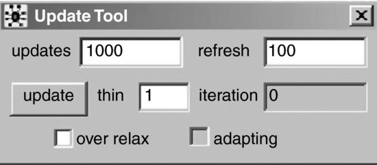
You then start the Markov chain going by going Model > Update (or equivalently ALT, then M, then U) and at which point a window (referred to as the Update Tool) as depicted in Figure 9.6 should appear. Clicking on update will cause the chain to go through a large number of states each time. In a simple example, the default number of states is likely (but not certain) to be enough. After you have done this, you should not close down this tool, because you will need it again later.
Figure 9.6 Update Tool.
The updating tool will cause the Markov chain to progress through a series of states, but will not sore any information about them, so once you have gone through an initial ‘burn-in’ so that (you hope) the chain has converged to equilibrium, you need to state which parameters you are interested in and what you want to know about them. You can do this by going Inference > Samples or by pressing ALT and then n (at least provided you no longer have text selected on your data input window). A window (referred to as the Sample Monitor Tool) depicted in Figure 9.7 will then appear. In the example, we are considering, you should enter y against node. The word set will then be highlighted and you should click on it. The space by node will again be blank, allowing you to enter further parameters in cases where you are interested in knowing about several parameters.
Figure 9.7 Sample Monitor Tool.
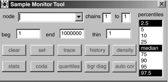
You should now cause the Markov chain to run through more states by using the Update Tool again, perhaps clicking update several times or altering the number against update to ensure that the averaging is taken over a large number of states. Then go back to the Sample Monitor Tool. You can select one of the parameters you have stored information about by clicking on the downward arrow to the right of node or by typing its name in the window there. Various statistics about the parameter or parameters of interest are then available. You can, for example, get a bar chart rather like the barplot obtained by ![]() by entering y against node and then clicking on density.
by entering y against node and then clicking on density.
9.7.4 The pump failure example revisited
WinBUGS is well suited to dealing with the example we considered in Sections 9.4 and 9.5 of pump failure data. A suitable program is as follows:
model
{
for (i in 1:k) {
a[i] ~ dchisqr(nu);
theta[i] < - a[i]/S0;
lambda[i] < - theta[i]*t[i]
Y[i] ~ dpois(lambda[i]);
}
nu ~ dexp(1.0);
S ~ dchisqr(1.0);
}
data;
list(k=10, Y=c(5,1,5,14,3,19,1,1,4,22),
t=c(94.320,15.720,62.880,125.760, 5.240,
31.440,1.048,1.048,2.096,10.480))
inits;
list(a=c(1,1,1,1,1,1,1,1,1,1),nu=2,S0=2)
9.7.5 DoodleBUGS
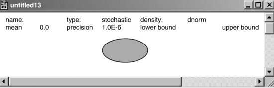
The inventors of WinBUGS recommend a graphical method of building up models. To start a Doodle go Doodle > New or press ALT and then D (followed by pressing RETURN twice). You should then see a blank window. Once you click anywhere on this window, you should see a picture like the one in Figure 9.8.
Figure 9.8 Doodle Screen.
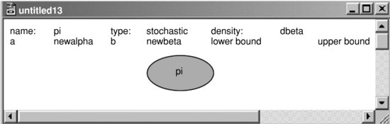
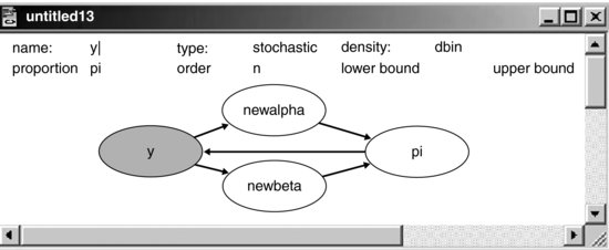
You can then adjust the parameters, so for example you can get a representation of the node pi in our simple example by altering the screen (beginning by clicking on density and altering that from the menu offered to dbeta) to look as in Figure 9.9.
Figure 9.9 Doodle for pi.
Clicking somewhere else on the window starts another node, until eventually you have nodes for pi and y (which have type set to stochastic) stochastic nodes) and for newalpha and newbeta (which have type set to logical and value set to y + alpha and n - y + beta, respectively). If you click on a previously formed node, then it is highlighted and you can alter its parameters. The fact that the parameters of one node are determined by the value of another is indicated by edges. Such an edge can be created when one node is highlighted by holding down CTRL and clicking on another node. The dependence of a node of type logical on another node will be indicated by a double arrow, while dependence on a stochastic node will be indicated by a single arrow. Nodes can be removed by pressing Delete while they are highlighted and edges can be removed as they were created (by ensuring that the node towards which the arrow comes is highlighted and then holding down CTRL and clicking on the node from which the arrow comes).
With the simple example we have been considering, the end result looks as indicated in Figure 9.10 (if the node for y is highlighted). You can then go Doodle > New or press ALT, then D, and then W or w to produce the code for the model as given earlier.
Figure 9.10 Doodle for the Casella–George example.
Working with DoodleBUGS is likely to be slower than writing the code directly, but if you do work this way you are less likely to end up with mystifying messages in the bottom left-hand corner of the WinBUGS window.
Of course, there are many more things you need to know if you want to work seriously with WinBUGS. The point of this subsection is to give you the self-confidence to get started with very simple examples, from which point you should be able to find out more for yourself. The program has a comprehensive online help system which is reasonably easy to follow. There is also a useful web resource that has been provided by Gillian Raab and can be found (among other places) at
9.7.6 coda
The acronym coda stands for Convergence Diagnostic and Output Analysis software, and is a menu-driven set of ![]() functions which serves as an output processor for the BUGS software. It may also be used in conduction with Markov chain Monte Carlo output from a user’s own programs, providing the output is formatted appropriately (see the coda manual for details). Using coda it is possible to compute convergence diagnostics and statistical and graphical summaries for the samples produced by the Gibbs sampler.
functions which serves as an output processor for the BUGS software. It may also be used in conduction with Markov chain Monte Carlo output from a user’s own programs, providing the output is formatted appropriately (see the coda manual for details). Using coda it is possible to compute convergence diagnostics and statistical and graphical summaries for the samples produced by the Gibbs sampler.
The inventors of WinBUGS remark, ‘Beware: MCMC sampling can be dangerous!’ and there is no doubt that they are right. You need to be extremely careful about assuming convergence, especially when using complex models, and for this reason it is well worth making use of the facilities which coda provides, although we shall not describe them here.
9.7.7 R2WinBUGS and R2OpenBUGS
It is now possible to run WinBUGS or OpenBugs directly from ![]() . To do this, it may be necessary, particularly in the case of WinBUGS, to run
. To do this, it may be necessary, particularly in the case of WinBUGS, to run ![]() as administrator, which is done by right clicking the icon for
as administrator, which is done by right clicking the icon for ![]() and choosing Run as administrator. Suppose we wish to run the program considered in Sections 9.4 and 9.7 concerning pumps in a nuclear plant. We first need a file called, for example, pumpsmodel.txt which contains the description of the model, in this case
and choosing Run as administrator. Suppose we wish to run the program considered in Sections 9.4 and 9.7 concerning pumps in a nuclear plant. We first need a file called, for example, pumpsmodel.txt which contains the description of the model, in this case
model;
{
y ~ dbin(pi,n)
pi ~ dbeta(newalpha,newbeta)
newalpha < - y + alpha
newbeta < - n - y + beta
}
We can then type into ![]()
library(R2WinBUGS)
windows(record=T)
data < - list(k=10, Y=c(5,1,5,14,3,19,1,1,4,22),
t=c(94.320,15.720,62.880,125.760,5.240,
31.440,1.048,1.048,2.096,10.480))
inits < - function() {
list(a=c(1,1,1,1,1,1,1,1,1,1), nu=2,S=2)
}
pumps.sim < - bugs(data, inits,
model.file=“pumpsmodel.txt”,
parameters=c(“theta”,“S”),
n.chains=3,n.iter=20000)
print(pumps.sim,digits=3)
plot(pumps.sim)
The results of a run with WinBUGS were as follows:
| System (i) | mean | s.d. |
| 1 | 0.058 | 0.025 |
| 2 | 0.102 | 0.079 |
| 3 | 0.088 | 0.038 |
| 4 | 0.116 | 0.032 |
| 5 | 0.602 | 0.325 |
| 6 | 0.610 | 0.138 |
| 7 | 0.829 | 0.664 |
| 8 | 0.827 | 0.705 |
| 9 | 1.472 | 0.727 |
| 10 | 1.978 | 0.409 |
It turns out that S0 has mean 2.269 and s.d. 1.151, but this is less important. We note that the results for the ![]() are very similar to those we found earlier in Section 9.4, although those for S are not quite so close.
are very similar to those we found earlier in Section 9.4, although those for S are not quite so close.
If we modify the call to bugs by adding in codaPkg=T, it is possible to investigate matters further using the package coda. A simple example of this is as follows:
. . . . . . . . . . . . . . . . . .
pumps.sim < - bugs(data, inits,
model.file=“pumpsmodel.txt”,
parameters=c(“theta”,“S”),
n.chains=3,n.iter=20000,
codaPkg=T)
codaobject < - read.bugs(pumps.sim)
plot(codaobject)
Figure 9.11 Plot of codaobject.
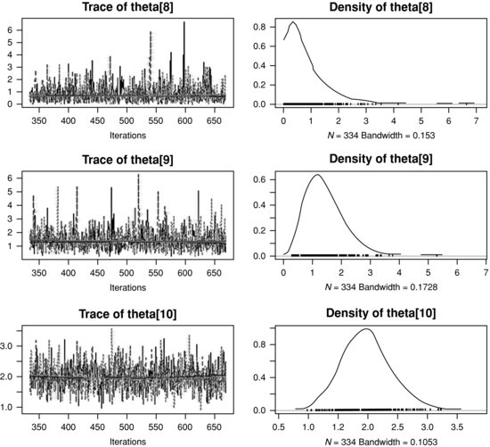
Part of the resulting plot can be seen in Figure 9.11. If you type codamenu(), then ![]() will respond
will respond
CODA startup menu
1: Read BUGS output files
2: Use an mcmc object
3: Quit
the response 2 followed by choosing codaobject as the name of saved object will allow further detailed analysis.
If you are running OpenBUGS you should use library (R2OpenBUGS) instead of library(R2WinBUGS). The package R2OpenBUGS will doubtless soon be available from the same source (CRAN) as other user-contributed packages for ![]() , but for the time being can be found at
, but for the time being can be found at
![]()
The manual is also available on the web site associated with this book.