9.8 Generalized linear models

9.8.1 Logistic regression

We shall illustrate this technique by considering some data from an experiment carried out by R. Norrell quoted by Weisberg (1985, Section 12.2). The matter of interest in this experiment was the effect of small electrical currents on farm animals, with the eventual goal of understanding the effects of high-voltage powerlines on livestock. The experiment was carried out with seven cows, and six shock intensities, 0, 1, 2, 3, 4 and 5 milliamps (shocks on the order of 15 milliamps are painful for many humans; see Dalziel et al. (1941). Each cow was given 30 shocks, five at each intensity, in random order. The entire experiment was then repeated, so each cow received a total of 60 shocks. For each shock the response, mouth movement, was either present or absent. The data as quoted give the total number of responses, out of 70 trials, at each shock level. We ignore cow differences and differences between blocks (experiments).

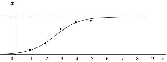
Our intention is to fit a smooth curve like the one shown in Figure 9.12 through these points in the same way that a straight line is fitted in ordinary regression. The procedure here has to be different because proportions, which estimate probabilities, have to lie between 0 and 1.

Figure 9.12 Logistic curve .

We define

and then observe that a suitable family of curves is given by

or equivalently

We have a binomial likelihood

(ignoring the binomial coefficients) with corresponding log-likelihood

where the binomial probabilities are related to the values of the explanatory variable xi by the above logistic equation. We then consider how to choose values of and so that the chosen curve best fits the data. The obvious general principle used by classical statisticians is that of maximum likelihood, and a simple iteration shows that with the data in the example, the maximum likelihood values are

There are nowadays many books which deal with logistic regression, usually from a classical standpoint, for example Kleinbaum (1994) and Hosmer and Lemeshow (1989).

In this book, we have tried to show how most of the standard statistical models can be fitted into a Bayesian framework, and logistic regression is no exception. All we need to do is to give and suitable prior distributions, noting that while we have no idea about the sign of , we would expect to be positive. Unfortunately, we cannot produce a model with conjugate priors, but we are able to use Gibbs sampling, and a suitable program for use in WinBUGS is as follows.

model;

{

    for (i in 1:6) {

     y[i] ～ dbin(pi[i],n[i])

     logit(pi[i]) < - beta0 + beta1*x[i]

    }

    beta0 ～ dnorm(0,0.001)

    beta1 ～ dgamma(0.001,0.001)

}

data;

list(y=c(0,9,21,47,60,63),

     n=c(70,70,70,70,70,70),

     x=c(0,1,2,3,4,5))

inits;

list(beta0=0,beta1=1)

A run of 5000 after a burn-in of 1000 resulted in a posterior mean of –3.314 for and of 1.251 for . Unsurprisingly, since we have chosen relatively uninformative priors, these are close to the maximum likelihood estimates.

Of course, a Bayesian analysis allows us to incorporate any prior information, we may have by taking different priors for and .

9.8.2 A general framework

We note that in Section 9.7, the parameter π of the binomial distribution is not itself linearly related to the explanatory variable x, but instead we have a relationship of the form

where in the case of logistic regression the function g, which is known as the link function is the logit function.

This pattern can be seen in various other models. For example, Gelman et al. (2004, Section 16.5) model the number yep of persons of ethnicity e stopped by the police in precinct p by defining nep as the number of arrests by the Division of Criminal Justice Services (DCJS) of New York State for that ethnic group in that precinct and then supposing that yep has a Poisson distribution

where

where the coefficients control for the ethnic group and the adjust for variation among precincts. Writing and taking explanatory variates such as where

this is a similar relationship to the one we encountered with logistic regression.

Similarly, a standard model often used for the table we encountered in 5.6 is to suppose that the entries in the four cells of the table each have Poisson distributions. More precisely, we suppose that the mean number in the top left-hand corner has some mean μ, that numbers in the second column have a mean α times bigger than corresponding values in the first column, and that numbers in the second row have means β times bigger than those in the first row (where, of course, α and β can be either greater or less than unity). It follows that the means in the four cells are μ, , and respectively. In this case we can regard the explanatory variables as the row and column in which any entry occurs and the Poisson distributions we encounter have means satisfying the equation

where

Further discussion of generalized linear models can be found in Dobson (2002) or McCullagh and Nelder (1989), and in a Bayesian context in Gelman et al. (2004, Chapter 16) and Dey et al. (2000).