
Chapter at a Glance

When you start Microsoft Excel 2010, the program presents a blank workbook that contains three worksheets. You can add or delete worksheets, hide worksheets within the workbook without deleting them, and change the order of your worksheets within the workbook. You can also copy a worksheet to another workbook or move the worksheet without leaving a copy of the worksheet in the first workbook. If you and your colleagues work with a large number of documents, you can define property values to make your workbooks easier to find when you and your colleagues attempt to locate them by using the Windows search facility.
Another way to make Excel easier to use is by customizing the Excel program window to fit your work style. If you have several workbooks open at the same time, you can move between the workbook windows quickly. However, if you switch between workbooks frequently, you might find it easier to resize the workbooks so they don’t take up the entire Excel window. If you do this, you just need to click the title bar of the workbook you want to modify to switch to it.
The Microsoft Office User Experience team has enhanced your ability to customize the Excel user interface. If you find that you use a command frequently, you can add it to the Quick Access Toolbar so it’s never more than one click away. If you use a set of commands frequently, you can create a custom ribbon tab so they appear in one place. You can also hide, display, or change the order of the tabs on the ribbon.
In this chapter, you’ll learn how to create and modify workbooks, create and modify worksheets, make your workbooks easier to find, and customize the Excel 2010 program window.
Note
Practice Files Before you can complete the exercises in this chapter, you need to copy the book’s practice files to your computer. The practice files you’ll use to complete the exercises in this chapter are in the Chapter08 practice file folder. A complete list of practice files is provided in Using the Practice Files at the beginning of this book.
Every time you want to gather and store data that isn’t closely related to any of your other existing data, you should create a new workbook. The default new workbook in Excel has three worksheets, although you can add more worksheets or delete existing worksheets if you want. Creating a new workbook is a straightforward process—you just click the File tab, click New, identify the type of workbook you want, and click the Create button.

When you start Excel, the program displays a new, blank workbook; you can begin to type data into the worksheet’s cells or open an existing workbook. In this book’s exercises, you’ll work with workbooks created for Consolidated Messenger, a fictional global shipping company. After you make changes to a workbook, you should save it to preserve your work.
Tip
Readers frequently ask, “How often should I save my files?” It is good practice to save your changes every half hour or even every five minutes, but the best time to save a file is whenever you make a change that you would hate to have to make again.
When you save a file, you overwrite the previous copy of the file. If you have made changes that you want to save, but you also want to keep a copy of the file as it was when you saved it previously, you can use the Save As command to specify a name for the new file.
You also can use the controls in the Save As dialog box to specify a different format for the new file and a different location in which to save the new version of the file. For example, Lori Penor, the chief operating officer of Consolidated Messenger, might want to save an Excel file that tracks consulting expenses as an Excel 2003 file if she needs to share the file with a consulting firm that uses Excel 2003.
After you create a file, you can add information to make the file easier to find when you use the Windows search facility to search for it. Each category of information, or property, stores specific information about your file. In Windows, you can search for files based on the file’s author or title, or by keywords associated with the file. A file tracking the postal code destinations of all packages sent from a vendor might have the keywords postal, destination, and origin associated with it.
To set values for your workbook’s built-in properties, you can click the File tab, click Info, click Properties, and then click Show Document Panel to display the Document Properties panel just below the ribbon. The standard version of the Document Properties panel has fields for the file’s author, title, subject, keywords, category, and status, and any comments about the file. You can also create custom properties by clicking the arrow located just to the right of the Document Properties label, and clicking Advanced Properties to display the Properties dialog box.

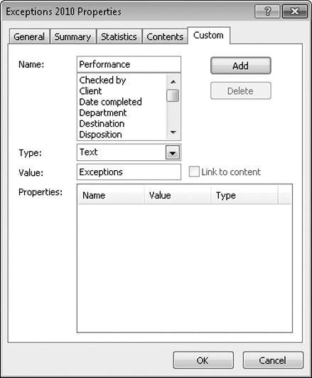
On the Custom page of the Properties dialog box, you can click one of the existing custom categories or create your own by typing a new property name in the Name field, clicking the Type arrow and selecting a data type (for example, Text, Date, Number, or Yes/No), selecting or typing a value in the Value field, and then clicking Add. If you want to delete an existing custom property, point to the Properties list, click the property you want to get rid of, and click Delete. After you finish making your changes, click the OK button. To hide the Document Properties panel, click the Close button in the upper-right corner of the panel.
In this exercise, you’ll create a new workbook, save the workbook with a new name, assign values to the workbook’s standard properties, and create a custom property.
Note
SET UP You need the ExceptionSummary_start workbook located in your Chapter08 practice file folder to complete this exercise. Start Excel, and open the ExceptionSummary_start workbook. Then follow the steps.
Click the File tab, and then click Close.
The ExceptionSummary_start workbook closes.
Click the File tab, and then click New.
The New Workbook page of the Backstage view appears.
Click Blank Workbook, and then click Create.
A new, blank workbook opens.
Navigate to your Chapter08 practice file folder. In the File name field, type Exceptions 2010.
Excel 2010 saves your work, and the Save As dialog box closes.
Click the File tab, click Info, click Properties, and then click Show Document Panel.
In the Keywords field, type exceptions, regional, percentage.
In the Category field, type performance.
Click the arrow at the right end of the Document Properties button, and then click Advanced Properties.
Click the Custom tab.
The Custom page is displayed.
Click the Add button, and then click OK.
On the Quick Access Toolbar, click the Save button to save your work.

Most of the time, you create a workbook to record information about a particular activity, such as the number of packages that a regional distribution center handles or the average time a driver takes to complete all deliveries on a route. Each worksheet within that workbook should represent a subdivision of that activity. To display a particular worksheet, just click the worksheet’s tab on the tab bar (just below the grid of cells).
In the case of Consolidated Messenger, the workbook used to track daily package volumes could have a separate worksheet for each regional distribution center. New Excel workbooks contain three worksheets; because Consolidated Messenger uses nine regional distribution centers, you would need to create six new ones. To create a new worksheet, click the Insert Worksheet button at the right edge of the tab bar.

After you decide what type of data you want to store on a worksheet, you should change the default worksheet name to something more descriptive. For example, you could change the name of Sheet1 in the regional distribution center tracking workbook to Northeast. When you want to change a worksheet’s name, double-click the worksheet’s tab on the tab bar to highlight the worksheet name, type the new name, and press Enter.
Another way to work with more than one worksheet is to copy a worksheet from another workbook to the current workbook. One circumstance in which you might consider copying worksheets to the current workbook is if you have a list of your current employees in another workbook. You can copy worksheets from another workbook by right-clicking the tab of the sheet you want to copy and, on the shortcut menu, clicking Move Or Copy to display the Move Or Copy dialog box.

After the worksheet is in the target workbook, you can change the worksheets’ order to make the data easier to locate within the workbook. To change a worksheet’s location in the workbook, you drag its sheet tab to the desired location on the tab bar. If you want to remove a worksheet from the tab bar without deleting the worksheet, you can do so by right-clicking the worksheet’s tab on the tab bar and clicking Hide on the context menu. When you want Excel to redisplay the worksheet, right-click any visible sheet tab and then click Unhide. In the Unhide dialog box, click the name of the sheet you want to display, and click OK.
To differentiate a worksheet from others, or to visually indicate groups or categories of work-sheets in a multiple-worksheet workbook, you can easily change the color of a worksheet tab. To do so, right-click the tab, point to Tab Color, and then click the color you want.
Tip
If you copy a worksheet to another workbook, and the destination workbook has the same Office Theme applied as the active workbook, the worksheet retains its tab color. If the destination workbook has another theme applied, the worksheet’s tab color changes to reflect that theme. For more information on Office themes, see Chapter 11.
If you determine that you no longer need a particular worksheet, such as one you created to store some figures temporarily, you can delete the worksheet quickly. To do so, right-click its sheet tab, and then click Delete.
In this exercise, you’ll insert and rename a worksheet, change a worksheet’s position in a workbook, hide and unhide a worksheet, copy a worksheet to another workbook, change a worksheet’s tab color, and delete a worksheet.
Note
SET UP You need the ExceptionTracking_start workbook located in your Chapter08 practice file folder to complete this exercise. Open the ExceptionTracking_start file, and save it as ExceptionTracking. Then follow the steps.
 On the tab bar, click the Insert Worksheet button.
A new worksheet is displayed.
Right-click the new worksheet’s sheet tab, and then click Rename.
Excel highlights the new worksheet’s name.
Type 2010, and then press Enter.
On the tab bar, double-click the Sheet1 sheet tab.
Excel highlights the worksheet’s name.
Type 2009, and then press Enter.
Right-click the 2009 sheet tab, point to Tab Color, and then, in the Standard Colors area of the color palette, click the green square.
Excel changes the 2009 sheet tab to green.
On the tab bar, drag the 2010 sheet tab to the left of the Scratch Pad sheet tab.
Right-click the 2010 sheet tab, and then click Hide.
Excel hides the 2010 worksheet.
Right-click the 2009 sheet tab, and then click Move or Copy.
Click the To book arrow, and then in the list, click (new book).
Select the Create a copy check box.
Click OK.
A new workbook opens, containing only the worksheet you copied into it.
 On the Quick Access Toolbar, click Save.
The Save As dialog box opens.
In the File name field, type 2009 Archive, and then press Enter.
Excel saves the workbook, and the Save As dialog box closes.
 On the View tab,
click the Switch Windows button, and then
click ExceptionTracking.
On the View tab,
click the Switch Windows button, and then
click ExceptionTracking.The ExceptionTracking workbook is displayed.
On the tab bar, right-click the Scratch Pad sheet tab, and then click Delete. In the dialog box that opens, click Delete to confirm the operation.
The Scratch Pad worksheet is deleted.
Right-click the 2009 sheet tab, and then click Unhide.
Click 2010, and then click OK.
The Unhide dialog box closes, and the 2010 worksheet is displayed in the workbook.


After you put up the signposts that make your data easy to find, you can take other steps to make the data in your workbooks easier to work with. For example, you can change the width of a column or the height of a row in a worksheet by dragging the column’s right border or the row’s bottom border to the desired position. Increasing a column’s width or a row’s height increases the space between cell contents, making your data easier to read and work with.
Tip
You can apply the same change to more than one row or column by selecting the rows or columns you want to change and then dragging the border of one of the selected rows or columns to the desired location. When you release the mouse button, all the selected rows or columns change to the new height or width.
Modifying column width and row height can make a workbook’s contents easier to work with, but you can also insert a row or column between cells that contain data to make your data easier to read. Adding space between the edge of a worksheet and cells that contain data, or perhaps between a label and the data to which it refers, makes the workbook’s contents less crowded. You insert rows by clicking a cell and clicking the Home tab on the ribbon. Then, in the Cells group, in the Insert list, click Insert Sheet Rows. Excel inserts a row above the row that contains the active cell. You insert a column in much the same way, by choosing Insert Sheet Columns from the Insert list. When you do this, Excel inserts a column to the left of the active cell.
When you insert a row, column, or cell in a worksheet that has had formatting applied, the Insert Options button appears. Clicking the Insert Options button displays a list of choices you can make about how the inserted row or column should be formatted. The following table summarizes your options.
|
Option |
Action |
|---|---|
|
Format Same As Above |
Applies the formatting of the row above the inserted row to the new row |
|
Format Same As Below |
Applies the formatting of the row below the inserted row to the new row |
|
Format Same As Left |
Applies the formatting of the column to the left of the inserted column to the new column |
|
Format Same As Right |
Applies the formatting of the column to the right of the inserted column to the new column |
|
Clear Formatting |
Applies the default format to the new row or column |
If you want to delete a row or column, right-click the row or column head and then, on the shortcut menu that appears, click Delete. You can temporarily hide rows or columns by selecting those rows or columns and then, on the Home tab, in the Cells group, clicking the Format button, pointing to Hide & Unhide, and then clicking either Hide Rows or Hide Columns. The rows or columns you selected disappear, but they aren’t gone for good, as they would be if you’d used Delete. Instead, they have just been removed from the display until you call them back. To return the hidden rows to the display, select the row or column headers on either side of the hidden rows or columns. Then, on the Home tab, in the Cells group, click the Format button, point to Hide & Unhide, and then click either Unhide Rows or Unhide Columns.
Important
If you hide the first row or column in a worksheet, you must click the Select All button in the upper-left corner of the worksheet (above the first row header and to the left of the first column header) or press Ctrl+A to select the entire worksheet. Then, on the Home tab, in the Cells group, click Format, point to Hide & Unhide, and then click either Unhide Rows or Unhide Columns to make the hidden data visible again.
Just as you can insert rows or columns, you can insert individual cells into a worksheet. To insert a cell, click the cell that is currently in the position where you want the new cell to appear. On the Home tab, in the Cells group, in the Insert list, click Insert Cells to display the Insert dialog box. In the Insert dialog box, you can choose whether to shift the cells surrounding the inserted cell down (if your data is arranged as a column) or to the right (if your data is arranged as a row). When you click OK, the new cell appears, and the contents of affected cells shift down or to the right, as appropriate. In a similar vein, if you want to delete a block of cells, select the cells, and on the Home tab, in the Cells group, in the Delete list, click Delete Cells to display the Delete dialog box—complete with options that enable you to choose how to shift the position of the cells around the deleted cells.
Tip
The Insert dialog box also includes options you can click to insert a new row or column; the Delete dialog box has similar options for deleting an entire row or column.
If you want to move the data in a group of cells to another location in your worksheet, select the cells you want to move and use the mouse pointer to point to the selection’s border. When the pointer changes to a four-pointed arrow, you can drag the selected cells to the desired location on the worksheet. If the destination cells contain data, Excel displays a dialog box asking whether you want to overwrite the destination cells’ contents. If you want to replace the existing values, click OK. If you don’t want to overwrite the existing values, click Cancel and insert the required number of cells to accommodate the data you want to move.
In this exercise, you’ll insert a column and row into a worksheet, specify insert options, hide a column, insert a cell into a worksheet, delete a cell from a worksheet, and move a group of cells within the worksheet.
Note
SET UP You need the RouteVolume_start workbook located in your Chapter08 practice file folder to complete this exercise. Open the RouteVolume_start workbook, and save it as RouteVolume. Then follow the steps.
On the May 12 worksheet, select cell A1.
 On the Home tab, in
the Cells group, click the Insert arrow, and then in the list, click
Insert Sheet Columns.
On the Home tab, in
the Cells group, click the Insert arrow, and then in the list, click
Insert Sheet Columns.A new column A appears.
In the Insert list, click Insert Sheet Rows.
A new row 1 appears.
 Click the Insert
Options button that appears
below the lower-right corner of the selected cell, and then click
Clear Formatting.
Click the Insert
Options button that appears
below the lower-right corner of the selected cell, and then click
Clear Formatting.Excel removes the formatting from the new row 1.
Right-click the column header of column E, and then click Hide.
On the tab bar, click the May 13 sheet tab.
The worksheet named May 13 appears.
Click cell B6.
 On the Home tab, in
the Cells
group, click the Delete arrow, and then
in the list, click Delete Cells.
On the Home tab, in
the Cells
group, click the Delete arrow, and then
in the list, click Delete Cells.If necessary, click Shift cells up, and then click OK.
The Delete dialog box closes and Excel deletes cell B6, moving the cells below it up to fill in the gap.
Click cell C6.
In the Cells group, in the Insert list, click Insert Cells.
If necessary, click Shift cells down, and then click OK.
The Insert dialog box closes, and Excel creates a new cell C6, moving cells C6:C11 down to accommodate the inserted cell.
In cell C6, type 4499, and then press Enter.
Select cells E13:F13.
Point to the border of the selected cells. When your mouse pointer changes to a four-pointed arrow, drag the selected cells to cells B13:C13.
The dragged cells replace cells B13:C13.


How you use Excel 2010 depends on your personal working style and the type of data collections you manage. The Excel product team interviews customers, observes how differing organizations use the program, and sets up the user interface so that many users won’t need to change it to work effectively. If you do want to change the Excel program window, including the user interface, you can. You can change how Excel displays your worksheets; zoom in on worksheet data; add frequently used commands to the Quick Access Toolbar; hide, display, and reorder ribbon tabs; and create custom tabs to make groups of commands readily accessible.
One way to make Excel easier to work with is to change the program’s zoom level. Just as you can “zoom in” with a camera to increase the size of an object in the camera’s viewer, you can use the zoom setting to change the size of objects within the Excel 2010 program window. For example, if Peter Villadsen, the Consolidated Messenger European Distribution Center Manager, displayed a worksheet that summarized his distribution center’s package volume by month, he could click the View tab and then, in the Zoom group, click the Zoom button to display the Zoom dialog box. The Zoom dialog box contains controls that he can use to select a preset magnification level or to type in a custom magnification level. He could also use the Zoom control in the lower-right corner of the Excel 2010 window.

Clicking the Zoom In control increases the size of items in the program window by 10 percent, whereas clicking the Zoom Out control decreases the size of items in the program window by 10 percent. If you want more fine-grained control of your zoom level, you can use the slider control to select a specific zoom level or click the magnification level indicator, which indicates the zoom percentage, and use the Zoom dialog box to set a custom magnification level.
The Zoom group on the View tab also contains the Zoom To Selection button, which fills the program window with the contents of any selected cells, up to the program’s maximum zoom level of 400 percent.
As you work with Excel, you will probably need to have more than one workbook open at a time. For example, you could open a workbook that contains customer contact information and copy it into another workbook to be used as the source data for a mass mailing you create in Microsoft Word 2010. When you have multiple workbooks open simultaneously, you can switch between them by clicking the View tab and then, in the Window group, clicking the Switch Windows button and clicking the name of the workbook you want to view.
You can arrange your workbooks within the Excel window so that most of the active workbook is shown but the others are easily accessible. To do so, click the View tab and then, in the Window group, click the Arrange All button. Then, in the Arrange Windows dialog box, click Cascade.

Many Excel 2010 workbooks contain formulas on one worksheet that derive their value from data on another worksheet, which means you need to change between two worksheets every time you want to see how modifying your data changes the formula’s result. However, an easier way to approach this is to display two copies of the same workbook simultaneously, displaying the worksheet that contains the data in the original window and displaying the worksheet with the formula in the new window. When you change the data in either copy of the workbook, Excel updates the other copy. To display two copies of the same workbook, open the desired workbook and then, in the View tab’s Window group, click New Window. Excel opens a second copy of the workbook. To display the workbooks side by side, on the View tab, in the Window group, click Arrange All. Then, in the Arrange Windows dialog box, click Vertical and then click OK.
If the original workbook’s name is Exception Summary, Excel 2010 displays the name Exception Summary:1 on the original workbook’s title bar and Exception Summary:2 on the second workbook’s title bar.

Note
Troubleshooting The appearance of buttons and groups on the ribbon changes depending on the width of the program window. For information about changing the appearance of the ribbon to match our images, see Modifying the Display of the Ribbon at the beginning of this book.
As you continue to work with Excel 2010, you might discover that you use certain commands much more frequently than others. If your workbooks draw data from external sources, for example, you might find yourself using the Refresh All button on the Data tab quite often than the program’s designers might have expected. You can make any button accessible with one click by adding the button to the Quick Access Toolbar, located just above the ribbon.
To add a button to the Quick Access Toolbar, display the Customize The Quick Access Toolbar page of the Excel Options dialog box. This page contains two panes. The pane on the left lists all of the controls that are available within a given category, and the pane on the right lists the controls currently displayed on the Quick Access Toolbar. In the Choose Commands From list, click the category that contains the control you want to add. Excel 2010 displays the available commands in the box below the Choose Commands From field. Click the control you want, and then click the Add button.
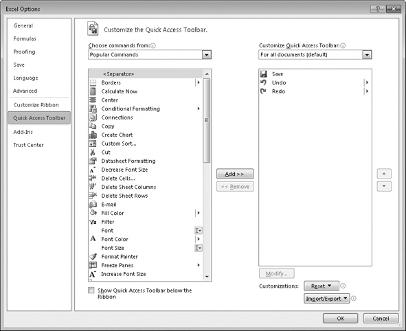
To remove a button from the Quick Access Toolbar, click the button’s name in the right pane, and then click the Remove button. When you’re done making your changes, click the OK button. If you prefer not to save your changes, click the Cancel button. If you saved your changes but want to return the Quick Access Toolbar to its original state, click the Reset button and then click either Reset Only Quick Access Toolbar, which removes any changes you made to the Quick Access Toolbar, or Reset All Customizations, which returns the entire ribbon interface to its original state.
You can also choose whether your Quick Access Toolbar changes affect all your workbooks or just the active workbook. To control how Excel applies your change, in the Customize Quick Access Toolbar list, click either For All Documents to apply the change to all of your workbooks or For Workbook to apply the change to the active workbook only.
If you’d like to export your Quick Access Toolbar customizations to a file that can be used to apply those changes to another Excel 2010 installation, click the Import/Export button and then click Export All Customizations. Use the controls in the dialog box that opens to save your file. When you’re ready to apply saved customizations to Excel, click the Import/Export button, click Import Customization File, select the file in the File Open dialog box, and click Open.
Excel 2010 enhances your ability to customize the entire ribbon by enabling you to hide and display ribbon tabs, reorder tabs displayed on the ribbon, customize existing tabs (including tool tabs, which appear when specific items are selected), and to create custom tabs.
To begin customizing the ribbon, click the File tab and then click Options. In the Excel Options dialog box, click Customize Ribbon to display the Customize The Ribbon page.
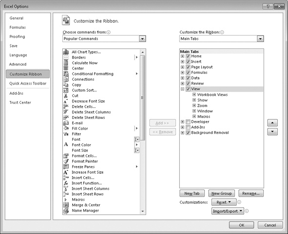
To select which tabs appear in the tabs pane on the right side of the screen, click the Customize The Ribbon field’s arrow and then click either Main Tabs, which displays the tabs that can appear on the standard ribbon; Tool Tabs, which displays the tabs that appear when you click an item such as a drawing object or PivotTable; or All Tabs.
Each ribbon tab’s name has a check box next to it. If a tab’s box is selected, then that tab appears on the ribbon. You can hide a tab by clearing the check box and bring it back by selecting the check box. You can also change the order in which the tabs are displayed on the ribbon. To do so, click the name of the tab you want to move and then click the Move Up or Move Down arrows to reposition the selected tab.
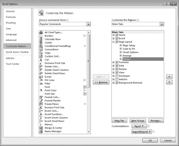
Just as you can change the order of the tabs on the ribbon, you can change the order of groups on a tab. For example, the Page Layout tab contains five groups: Themes, Page Setup, Scale To Fit, Sheet Options, and Arrange. If you use the Themes group infrequently, you could move the group to the right end of the tab by clicking the group’s name and then clicking the Move Down button until the group appears in the desired position.
To remove a group from a built-in ribbon tab, click the name of the group in the right pane and click the Remove button. If you remove a group from a built-in tab and later decide you want to put it back on the tab, display the tab in the right pane. Then, click the Choose Commands From field’s arrow and click Main Tabs. With the tab displayed, in the left pane, click the expand control (which looks like a plus sign) next to the name of the tab that contains the group you want to add back. You can now click the name of the group in the left pane and click the Add button to put the group back on the selected ribbon tab.
The built-in ribbon tabs are designed efficiently, so adding new command groups might crowd the other items on the tab and make those controls harder to find. Rather than adding controls to an existing ribbon tab, you can create a custom tab and then add groups and commands to it. To create a custom ribbon tab, click the New Tab button on the Customize The Ribbon page of the Excel Options dialog box. When you do, a new tab named New Tab (Custom), which contains a group named New Group (Custom), appears in the tab list.
You can add an existing group to your new ribbon tab by clicking the Choose Commands From field’s arrow, selecting a collection of commands, clicking the group you want to add, and then clicking the Add button. You can also add individual commands to your ribbon tab by clicking a command in the command list and clicking the Add button. To add a command to your tab’s custom group, click the new group in the right tab list, click the command in the left list, and then click the Add button. If you want to add another custom group to your new tab, click the new tab, or any of the groups within that tab, and then click New Group.
The New Tab (Custom) name doesn’t tell you anything about the commands on your new ribbon tab, so you can rename it to reflect its contents. To rename any tab on the ribbon, display the Customize The Ribbon page of the Excel Options dialog box, click the tab you want to modify, and then click the Rename button. Type the tab’s new name in the Rename dialog box, and click OK. To rename any group on the ribbon, click the name of the group, and then click Rename. When you do, a different version of the Rename dialog box appears. Click the symbol that you want to use to represent the group on the ribbon, type a new name for the group in the Display Name box, and click OK.

If you’d like to export your ribbon customizations to a file that can be used to apply those changes to another Excel 2010 installation, click the Import/Export button and then click Export All Customizations. Use the controls in the dialog box that opens to save your file. When you’re ready to apply saved customizations to Excel, click the Import/Export button, click Import Customization File, select the file in the File Open dialog box, and click Open.
When you’re done customizing the ribbon, click the OK button to save your changes or click Cancel to keep the user interface as it was before you started this round of changes. You can also change a ribbon tab, or the entire ribbon, back to the state it was in when you installed Excel. To restore a single ribbon tab, click the tab you want to restore, click the Reset button, and then click Reset Only Selected Ribbon Tab. To restore the entire ribbon, including the Quick Access Toolbar, click the Reset button and then click Reset All Customizations.
You can increase the amount of space available inside the program window by hiding the ribbon, the formula bar, or the row and column labels.
To hide the ribbon, double-click the active tab label. The tab labels remain visible at the top of the program window, but the tab content is hidden. To temporarily redisplay the ribbon, click the tab label you want. Then click any button on the tab, or click away from the tab, to rehide it. To permanently redisplay the ribbon, double-click any tab label.
To hide the formula bar, clear the Formula Bar check box in the Show/Hide group on the View tab. To hide the row and column labels, clear the Headings check box in the Show/Hide group on the View tab.
In this exercise, you’ll change your worksheet’s zoom level, zoom in to emphasize a selected cell range, switch between multiple open workbooks, cascade multiple open workbooks within the Excel program window, add a button to the Quick Access Toolbar, and customize the ribbon.
Note
SET UP You need the PackageCounts_start and MisroutedPackages_start workbooks located in your Chapter08 practice file folder to complete this exercise. Open the PackageCounts_start and MisroutedPackages_start workbooks, and save them as PackageCounts and MisroutedPackages, respectively. Then follow the steps.
In the MisroutedPackages workbook, in the lower-right corner of the Excel 2010 window, click the Zoom In control five times.
The worksheet’s zoom level changes to 150%.
Select cells B2:C11.
 On the View tab,
in the Zoom group, click the Zoom to Selection button.
On the View tab,
in the Zoom group, click the Zoom to Selection button.Excel displays the selected cells so they fill the program window.
Click 100%, and then click OK.
The worksheet returns to its default zoom level.
- On the View tab,
in the Window group, click the
Switch Windows
button, and then click
PackageCounts.
The PackageCounts workbook opens.
 On the View tab,
in the Window group, click the
Arrange All button.
On the View tab,
in the Window group, click the
Arrange All button.Click Cascade, and then click OK.
Excel cascades the open workbook windows within the program window.
Click the File tab, and then click Options.
The Excel Options dialog box opens.
Click Quick Access Toolbar.
Click the Choose commands from arrow, and then in the list, click Review Tab.
The commands in the Review Tab category appear in the command list.
Click the Spelling command, and then click Add.
Excel adds the Spelling command to the Quick Access Toolbar.
Click Customize Ribbon.
The Customize The Ribbon page of the Excel Options dialog box appears.
 If necessary, click the Customize the Ribbon box’s arrow and click
Main Tabs.
In the right tab list, click the Review tab and then click the Move Up button three times.
If necessary, click the Customize the Ribbon box’s arrow and click
Main Tabs.
In the right tab list, click the Review tab and then click the Move Up button three times.Excel moves the Review tab between the Insert and Page Layout tabs.
Click the New Tab button.
A tab named New Tab (Custom) appears below the most recently active tab in the Main Tabs list.
Click the New Tab (Custom) tab name, click the Rename button, type My Commands in the Display Name box, and click OK.
The new tab’s name changes to My Commands.
Click the New Group (Custom) group and then click Rename. In the Rename dialog box, click the icon that looks like a paint palette (second row, fourth from the right). Then type Formatting in the Display name box, and click OK.
The new group’s name changes to Formatting.
In the right tab list, click the My Commands tab name. Then, on the left side of the dialog box, click the Choose Commands From box’s arrow and click Main Tabs.
The Main Tabs group of ribbon tabs appears in the left tab list.
In the left tab list, click the Home tab’s expand control, click the Styles group’s name, and then click the Add button.
The Styles group is added to the My Commands tab.
In the left tab list, under the Home tab, click the Number group’s expand control.
The commands in the Number group appear.
In the right tab list, click the Formatting group you created earlier. Then, in the left tab list, click the Number Format item and click the Add button.
Excel 2010 adds the Number Format item to the Formatting custom group.
Click OK to save your ribbon customizations, and then click the My Commands tab on the ribbon.


Save your work whenever you do something you’d hate to have to do again.
Assigning values to a workbook’s properties makes it easier to find your workbook using the Windows search facility.
Be sure to give your worksheets descriptive names.
If you want to use a worksheet’s data in another workbook, you can send a copy of the worksheet to that other workbook without deleting the original worksheet.
You can delete a worksheet you no longer need, but you can also hide a worksheet in the workbook. When you need the data on the worksheet, you can unhide it.
You can save yourself a lot of bothersome cutting and pasting by inserting and deleting worksheet cells, columns, and rows.
Customize your Excel 2010 program window by changing how it displays your workbooks, zooming in on data, adding frequently used buttons to the Quick Access Toolbar, and rearranging or customizing the ribbon to meet your needs.