8 Smart Arrays

A smart antenna adapts its receive and/or transmit pattern characteristics in response to the signals in the environment. At least two different antennas comprise a smart antenna, usually in the form of an antenna array. The amplitude and phase of the received signals are weighted and summed in such a way as to meet some desired performance expectation. This chapter describes several different kinds of smart antennas. The first is a retrodirective array that retransmits a received signal back in the same direction. Another type of smart array finds the angular location of signals in the environment, so they are called direction finding (DF) arrays. The simple Adcock array was presented in Chapter 2. In this chapter, arrays that can automatically detect many signals are presented. Antennas that automatically reject interference while still receiving the desired signal are important in an environment with many signals. It may place a null in the direction of an interference source or steer the main beam in the direction of a desired signal. The sidelobe canceller was the first approach to placing a null in the sidelobe of the array pattern. This concept was generalized to the adaptive array that requires signal measurements at each element. A digital beamformer is ideal for this approach due to the complete control of the signals at the elements. It is also possible to adaptively place nulls using a conventional corporate-fed array by using an optimization algorithm to minimize the total power output. The main beam is not nulled, because only some of the elements or a few bits in the amplitude/phase controls. Finally, the ultimate smart antenna has an adaptive transmit and adaptive receive array. MIMO (multiple input multiple output) communications systems have adaptive transmit and receive antennas. All of these approaches are described in this chapter.

8.1. RETRODIRECTIVE ARRAYS

Ideas for actual smart antennas did not originate until the 1950s when Van Atta invented retroirective and redirective arrays [1]. The Van Atta array receives and reradiates an incident wave in a predetermined direction with respect to the incident angle. Usually, this type of array adjusts the phase and may also amplify the received signals such that it retransmits in the direction of the incident field. This array operates similar to a dihedral or trihedral corner reflector in which the signal reflects back to the transmitter. Less common is the redirective array that retransmits the received signal in a direction different from the received direction.

Figure 8.1. Diagram of a Van Atta arrays, (a) Retrodirective array, (b) Redirective array.

Figure 8.1a is a diagram of a Van Atta retrodirective array. Symmetric elements about the center of the array are connected by a transmission line. All transmission lines connecting the elements are of identical length, so the relative phase of the signals is maintained. Upon transmit, the received signals are now on opposite sides of the array, so the transmitted wavefront returns from direction that it came. Figure 8.1a follows the paths of signals received and transmitted by the end elements. Figure 8.1b is a redirective Van Atta array where the received signal is retransmitted in a different direction.

The received signals at the elements of an isotropic Van Atta array are given by

where u_i, is the angle of the incident field. Since the transmission lines are all the same length (l), a constant phase is added to the signals. By the time they reach the element on the other side of the array (assuming no loss), the signals are given by

The phase shift between two adjacent elements in (8.2) is given by

which implies that the transmit beam points in the same direction as the incident plane wave: u_i.

Figure 8.2. Active element in a retrodirective array.

Since the Van Atta array requires that symmetric elements in the array be connected by equal length transmission lines, this type of array will not work with nonplanar arrays or nonplanar wavefronts. An alternative is to have each element receive and then modify and retransmit the received signal in order to accommodate curved apertures, near-field sources, and broadband signals. An active retrodirective array has circulators and amplifiers in the transmission paths between elements as shown in Figure 8.2. This type of retrodirective array has a radar cross section given by [2]

where N is the number of elements in the array, G_e is element gain, and G_a is amplifier gain minus losses of circulators. An active retrodirective array is useful as a transponder or as an enhanced radar target (Figure 8.2) [3]. This beacon automatically replies in the direction of the interrogation signal without prior knowledge of the interrogator location.

One approach to an active retrodirective array uses phase conjugation at the elements [4]. When a local oscillator (LO) heterodynes its signal with the RF signal, the following signal results [5]:

If the LO frequency is double the RF frequency, then the lower sideband is the phase conjugation of the received signal. The high sideband signal is easily filtered out, so it is not retransmitted. This approach becomes less practical as f_RF gets higher, because the LO source must operate at double f_RF, making the LO source very expensive [6].

Figure 8.3. Diagram of an array with a receiver at each element.

Retrodirective arrays have applications in radio-frequency identification (RFID) [7], wireless communications, and RF transponders. All these applications require a signal be returned to the source. The signal may be amplified and the frequency or polarization may be slightly altered to distinguish it from the original signal. It is possible to have a two-dimensional retrodirective array that responds to both azimuth and elevation angles [8, 9].

8.2. ARRAY SIGNALS AND NOISE

Element signals are down-converted and sent to the computer (Figure 8.3). A computer forms an array steering vector to control the pattern. The time-dependent array output is

where

and w is the element weight vector, s(t) is the signal vector, A(θ_m) is the array steering vector, and N(t) is the noise vector. Neither the element weights nor the array steering vectors are time-dependent. The signal vector is the amplitude of the plane wave incident on the array at θ_m:

The signals have a bandpass spectrum modulated by a suppressed carrier frequency due to the time harmonic field representations. Some possible signal representations to use in a computer model are

The function randn returns a normally distributed random matrix, and rand returns a uniformly distributed random matrix with N rows and K columns. Gaussian white noise has a flat power spectrum having an amplitude . It is calculated using

The array steering vector, A(θ_m), contains the phase of plane wave m at each of the elements. It varies with incident angle but not time. The steering vectors for each of the M incident signals are placed in the columns of a matrix, A.

The output power is proportional to the array output squared.

where R_T is the covariance matrix, † is the complex conjugate transpose of the vector, and E{} is the expected value. In this chapter, we assume that all the signals are zero mean, stationary processes, so the covariance matrix is also the correlation matrix.

An estimate of the correlation matrix built from the signal and noise samples at K time intervals is given by

When the signal and noise are uncorrelated and enough samples are taken, then

Since the noise is uncorrelated from element to element, the noise correlation matrix off-diagonal elements are zero when K is large enough, and the diagonal elements are the noise variance.

Eigenvectors and eigenvalues of the correlation matrix correspond to the received signals and noise. An eigen decomposition of the correlation matrix is written as

where V_λ is a matrix whose columns are the eigenvectors, λ_n is an eigenvalue associated with the eigenvector in column n, and I_N is an N × N identity matrix. The largest eigenvalues correspond to the signals, while the rest are associated with the noise. The signal eigenvectors span the signal subspace, while the noise eigenvectors span the noise subspace. All the noise eigenvalues equal the noise variance, . They are not a function of angle. The signal eigenvalues, however, are a function of signal direction and signal amplitude. M uncor-related signals incident on an N element array (N > M) produces M signal eigenvalues and N – M noise eigenvalues. Element patterns and element spacing affect the eigenvalues of the correlation matrix [10].

The signal eigenvectors associated with the correlation matrix are the array weights that have beams in the directions of the signals. The noise eigenvectors associated with the correlation matrix are the array weights that have nulls in the directions of the signals. Eigenvalues are related to the signal and noise powers. Array factors associated with eigenvector weights are called eigenbeams [11]. For a uniform linear array along the x axis, eigenbeam m is calculated from eigenvector m by

The correlation matrix is the crux of most adaptive array schemes, so it is worth further investigation before presenting any adaptive antenna algorithms. A few examples will help.

Example. Compare the eigenvectors and eigenvalues of the correlation matrix of a 4-element uniform array with half-wavelength spacing under the following scenarios:

1. 1-V/m plane wave incident at 20°.
2. 1-V/m plane wave incident at −50° and a 1-V/m plane wave incident at 30°.
3. 1-V/m plane wave incident at −50° and a 2-V/m plane wave incident at 30°.

Assume σ_noise = 0.01.

1. The eigenvectors and eigenvalues associated with 1-V/m plane wave incident at 20° are displayed in Table 8.1. The first three eigenvalues equal σ_noise while the last one, corresponding to the signal, is much higher. The amplitude of V₄ is uniform while the phase has a progression equal to the phase needed to steer the eigenbeam to 20°.
   

   

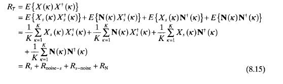
   Figure 8.4 is a plot of the four eigenbeams. The signal eigenbeam is a uniform array factor steered to 20°. The noise eigenbeams all have nulls at 20°.

2. The eigenvectors and eigenvalues associated with 1-V/m plane wave incident at −50° and a 1-V/m plane wave incident at 30° are displayed in Table 8.2. The first two eigenvalues are equal to σ_noise while the second two, corresponding to the signals, are much higher. The eigenbeams associated with V₃ and V₄ have peaks at −50° and 30° because
   

   TABLE 8.1. Eigen Analysis of the Correlation Matrix for a 4-Element Uniform Array with a 1-V/m Plane Wave Incident at 20°

   

   

   Figure 8.4. Plot of eigenbeams for the 4-element uniform array with one signal present at θ = 20°.

   TABLE 8.2. Eigen Analysis of the Correlation Matrix for a 4-Element Uniform Array with a 1-V/m Plane Wave Incident at −50° and a 1-V/m Plane Wave Incident at 30°

   

   

   Figure 8.5 is a plot of the four eigenbeams. The noise eigenbeams all have nulls at −50° and 30°.

   

   Figure 8.5. Plot of eigenbeams for the 4-element uniform array with 1-V/m plane wave incident at −50° and a 1-V/m plane wave incident at 30°.

   TABLE 8.3. Eigen Analysis of the Correlation Matrix for a 4-Element Uniform Array with a 1-V/m Plane Wave Incident at −50° and a 2-V/m Plane Wave Incident at 30°

   

3. The eigenvectors and eigenvalues associated with 1-V/m plane wave incident at −50° and a 2-V/m plane wave incident at 30° are displayed in Table 8.3. As in Table 8.2, the first two eigenvalues are equal to σ_noise while the second two, corresponding to the signals, are much higher. The eigenbeams associated with V3 and V4 have peaks at −50° and 30°. This time, the peaks in the patterns are not of equal height: One beam has a higher peak at −50° and the other beam has a higher peak at 30°. Figure 8.6 is a plot of the four eigenbeams. The noise eigenbeams all have nulls at −50° and 30°.

Figure 8.6. Plot of eigenbeams for the 4-element uniform array with 1-V/m plane wave incident at −50° and a 2-V/m plane wave incident at 30°.

Example. The eigenvalues of the correlation matrix relate to the strength of the signals, the noise, and the separation between the signals. A 4-element uniform array with half-wavelength spacing has up to two signals incident upon it. Plot the relationship between the eigenvalues and the standard deviation of the noise, the eigenvalues and the separation distance between two signals of equal strength, and the eigenvalues and the ratio of the strength of two signals.

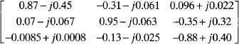
When two signals of strength 1-V/m modeled by (8.9) are incident at 0° and 40° with σ_noise = 0.01, the correlation matrix is

and has the eigenvalues [0.0078 0.0102 3.3786 4.5022]^T.

The two signals correspond to the two largest eigenvalues. Increasing σ_noise from 0 to 1.98 when only one signal is present at θ₁ = 0° causes the eigenvalues to increase as shown in Figure 8.7. The eigenvalues are sorted from the largest, λ₁ (signal), to the smallest, λ₄. As σ_noise increases, so do all the eigenvalues. Variations in the eigenvalues increase as σ_noise increases.

Figure 8.7. Plot of eigenvalues versus σ_noise for the 4-element uniform array with one signal present at θ₁ = 0°.

Figure 8.8. Plot of eigenvalues versus angular separation distance between two equally weighted signals are incident on the 4-element array.

Two signals incident on the array (σ_noise = 0.01) with one incident at θ₁ = 0° and the other incident at −49.5° ≤ θ₂ ≤ 49.5° results in the eigenvalue plot shown in Figure 8.8. λ₁ begins to increase and λ₂ decrease as s₂ enters the main beam. When both signals are incident at θ = 0°, then λ₁ approximately doubles and λ₂ is approximately zero and is indistinguishable from the noise eigenvalues. Two signals are incident on the array (σ_noise = 0.01) with s₁ = 1 incident at θ₁ = 0° and 0 ≤ s₂ ≤ 1.98s₁ incident at θ₂ = 40°. Figure 8.9 shows the eigenvalues graphed as a function of s₂/s₁. When s₂ = 0, then λ₁ = 4 and λ₂ = 0. Increasing s₂ until it equals s₁ results in λ₁ staying approximately constant but λ₂ increases. When s₂ > s₁ then λ₂ stays approximately constant while λ₁ increases. The largest eigenvalue always corresponds to the most powerful signal.

Figure 8.9. Plot of eigenvalues versus signal strength ratio for two equally weighted signals are incident on the 4-element array.

The same principles for forming the correlation matrix for linear arrays apply to arbitrary arrays as well. The array steering vector becomes a function of θ and rather than a single angle.

8.3. DIRECTION OF ARRIVAL ESTIMATION

Direction finding was already introduced in Chapter 2. This chapter presents several signal processing algorithms for automatically determining the locations of the signals incident upon an array [12]. All the algorithms presented here assume that a calibrated receiver is at each element in the array. A calibrated receiver ensures that the relative signal amplitudes and phases are maintained between the elements. Otherwise, the correlation matrix would not be correct, so the eigenvectors and eigenvalues would be wrong.

Since an array’s ability to resolve signals depends upon the beamwidth of the array, other high-resolution algorithms have been developed, so that even small arrays can resolve closely spaced signals. They resolve N − 1 signals by using narrow nulls in place of the wide main beam. These are also sensitive to noise, however.

8.3.1. Periodogram

One way to determine the signals present in the vicinity of an array is to scan the beam over the region of interest and plot the output power as a function of angle. The relative array output power as a function of angle can be found by

where the uniform array steering vector is given by

A plot of the output power versus angle is known as a periodogram. Resolving closely spaced signals is limited by the array beamwidth.

Example. Demonstrate the effect of separation angle between two sources using an 8-element uniform array with λ/2 spacing.

When θ₁ = −30° and θ₂ = 30°, two distinct peaks occur in the periodogram (Figure 8.10). Moving θ₁ to 10° still maintains two distinct peaks, but the dip between them has become shallow. When θ₁ is at 20°, then only one peak occurs halfway between the two signals. Thus, if the signals are close together, then they appear as one signal from a direction between the two signals.

Figure 8.10. Plot of the periodogram of the 8-element uniform array when θ₁ = −30°, 10°, 20°, and θ₂ = 30°.

8.3.2. Capon’s Minimum Variance

The periodogram basically uses the main beam of the array to determine signal locations. Since the main beam is wide, especially for small arrays, the ability to separate multiple signals or accurately locate a signal is not very good. Using nulls to locate signals is much more desirable, because the nulls have a narrow angular extent. Capon’s method is the maximum likelihood estimate of the power arriving from a desired direction while all the other sources are considered interference [13]. Thus, the goal is to minimize the output power while forcing the desired signal to remain constant. The signal-to-interference ratio is maximized by the array weights

The resulting spectrum is given by

Capon’s method does not work well when the signals are correlated.

Example. An 8-element uniform array with λ/2 spacing has three signals incident upon it: s₁(−60°) = 1, s₂(0°) = 2, and s₃(10°) = 4. Find the Capon spectrum.

Figure 8.11 shows the result of Capon’s method superimposed on the periodogram. Capon’s method can better distinguish between two closely spaced sources and the spectrum between the source peaks is very low. The periodogram cannot separate the signals at 0° and 10°.

8.3.3. MUSIC Algorithm

MUSIC is an acronym for MUltiple SIgnal Classification [14]. MUSIC assumes the noise is uncorrelated and the signals are either uncorrelated or mildly correlated. When the array calibration is perfect and the signals uncorrelated, then the MUSIC algorithm can accurately estimate the number of signals, the angle of arrivals, and the signal strengths [15]. The MUSIC spectrum is given by

where V_λ is a matrix whose columns contain the eigenvectors of the noise subspace. The eigenvectors of the noise subspace correspond to the N − N_s smallest eigenvalues of the correlation matrix.

Figure 8.11. Plot of the 4-element uniform array Capon spectrum with three signals present.

Figure 8.12. Plot of the 8-element uniform array MUSIC spectrum with three signals present.

Example. An 8-element uniform array with λ/2 spacing has three signals incident upon it: s₁(−60°) = 1, s₂(0°) = 2, and s₃(10°) = 4. Find the MUSIC spectrum.

Figure 8.12 shows the MUSIC spectrum superimposed on the periodogram. MUSIC easily distinguishes between two closely spaced sources and the spectrum between the source peaks is lower than in the Capon spectrum.

The MUSIC algorithm is not very robust, so many improvements have been proposed. One popular modification, called root-MUSIC, accurately locates the direction of arrival by finding the roots of the array polynomial [16]. The denominator of (8.24) can be written as

where

Z = e^{jknd sin θ}

sum of nth diagonal of matrix

The summation in (8.25) is over the diagonals of . Coefficient n is the sum of the elements in diagonal n. Roots of the polynomial, z_m, close to the unit circle correspond to the poles of the MUSIC spectrum. Solving for the angle of the phase of the roots of the polynomial in (8.25) produces

Roots close to the unit circle correspond to actual signals while the rest are spurious. The has 2N − 1 diagonals, so the polynomial has 2N − 2 roots.

Example. An 8-element uniform array with λ/2 spacing has three signals incident upon it: s₁(−60°) = 1, s₂(0°) = 2, and s₃(10°) = 4. Find the location of the signals using the root MUSIC algorithm.

The magnitude and angle of the roots are calculated using |z_m| and (8.26) to get the values in Table 8.4. The three signal directions are accurately identified as the roots that lie on the unit circle (|z_m| ≈ 1). A unit circle plot of all 14 roots is shown in Figure 8.13.

TABLE 8.4. The Roots Found Using Root MUSIC^a

^aThe ones close to the unit circle represent the correct signal directions.

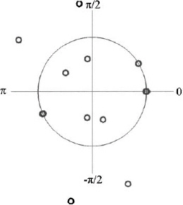
Figure 8.13. Unit circle representation of all the roots found using root MUSIC.

8.3.4. Maximum Entropy Method

The maximum entropy method (MEM) is also called the all-poles model or the autoregressive model. MEM is based on a rational function model of the spectrum having all poles and no zeros [17]. Hence, it can accurately reproduce sharp resonances in the spectrum. The MEM spectrum is given by [18]

where n is the nth column of the inverse correlation matrix. The selection of n gives slightly different results.

Example. An 8-element uniform array with λ/2 spacing has three signals incident upon it: s₁(−60°) = 1, s₂(0°) = 2, and s₃(10°) = 4. Find the MEM spectrum.

Figure 8.14 shows the MEM spectrum superimposed on the periodogram. MEM has even sharper spectral lines than the MUSIC spectrum.

8.3.5. Pisarenko Harmonic Decomposition

The smallest eigenvector (λ_N) minimizes the mean squared error of the array output with the constraint that the norm of the weight vector equals one. The Pisarenko harmonic decomposition (PHD) spectrum is [19]

Figure 8.14. Plot of the 4-element uniform array MEM spectrum with three signals present.

Figure 8.15. Plot of the 4-element uniform array PHD spectrum with three signals present.

Example. An 8-element uniform array with λ/2 spacing has three signals incident upon it: s₁(−60°) = 1, s₂(0°) = 2, and s₃(10°) = 4. Find the PHD spectrum.

Figure 8.15 shows the PHD spectrum superimposed on the periodogram. PHD has very sharp spectral lines like MEM.

8.3.6. ESPRIT

ESPRIT is an acronym for Estimation of Signal Parameters via Rotational Invariance Techniques [20]. It is based upon breaking an N-element uniform linear array into two overlapping subarrays with N − 1 elements. One subarray starts at the left end of the array, and the other starts at the right end of the array. The N − 2 shared elements in the middle are called matched pairs. ESPRIT makes use of the phase displacement between the two subarrays to calculate the angle of arrivals for the signals. The signals at the elements in the two subarrays are written as

where the diagonal matrix, Φ has elements Φ_m,m = e^{jkd sin θ_m}. The eigenvectors of the full array are in matrix V_λ A new N × M matrix with only the signal eigenvectors is defined by

The first N − 1 rows are associated with the first subarray, while the last N − 1 rows are associated with the second subarray. A matrix Ψ relates the two subarray eigenvector matrixes by

Solving for Ψ and equating its eigenvalues to Φ results in the signal angle estimates of

where = eigenvalues of Ψ.

Example. An 8-element uniform array with λ/2 spacing has three signals incident upon it: s₁(−6Q°) = 1, s₂(0°) = 2, and s₃(10°) = 4. Estimate the incident angles using ESPRIT.

First calculate the correlation matrix, then find the eigenvectors associated with the three signals.

Next, compute Ψ to get

The eigenvalues of ψ are found and substituted into (8.32) to find an estimate of the angle of arrival.

θ_m = [−59.91° 0.06° 10.0°]

8.3.7. Estimating and Finding Sources

Many of the direction finding algorithms need to know the exact number of sources incident upon the array. One way is to just pick the eigenvalues that exceed some threshold set above the noise. The number of eigenvalues that exceed the threshold equals the number of sources. One algorithm for estimating M is as follows [21]:

1. Estimate the correlation matrix from K time samples.
2. Find and sort the eigenvalues (λ₁ > λ₂ > ··· > λ_N).
3. Find M that minimizes [21]

where

AIC = Akaike’s information criterion

MDL = minimum description length

8.4. ADAPTIVE NULLING

As the wireless users crowd the frequency spectrum, interference becomes more common. When the main beam gain times the desired signal is less than the sidelobe gain times the interference signal, then the interference overwhelms the desired signal. An adaptive antenna adjusts its antenna pattern to steer the main beam in the direction of the desired signal while placing nulls in the direction of the interference. The original adaptive antenna, called a sidelobe canceler, was invented by Howells and Applebaum [22]. It was mainly intended for radar systems. A similar adaptive algorithm was independently developed by Widrow [23]. This least mean square (LMS) algorithm became the canonical adaptive algorithm primarily intended for communications systems. Many signal processing algorithms have their roots in the LMS algorithm. They all require a calibrated receiver at each element in the array. Another approach that relies on random search algorithms works with a corporate fed array with one receiver [24]. These approaches minimize the output power of the array. If only a few of the elements or the least significant bits of the weights are used to perform the nulling, then nulls cannot be placed in the main beam but can be placed in the sidelobes [25]. The advent of global optimization algorithms have made this approach more attractive [26].

This section is divided into three parts. First, the radar approaches called sidelobe blanking and sidelobe canceling are presented. These techniques do not require a pilot signal or replica of the desired receive signal to work. The second set of algorithms rely upon the signal correlation matrix. They are similar to the direction finding algorithms, except one of the signal steering vectors corresponds to the desired signal, while the others correspond to the interference. Some examples that demonstrate the operation of these types of algorithms are presented. Finally, the random search type algorithms are presented, because of their attractive minimal hardware requirements.

8.4.1. Sidelobe Blanking and Canceling

A sidelobe blanker eliminates unwanted interference entering the sidelobes of a radar array [27] (Figure 8.16). It consists of a high-gain radar antenna and a lower-gain auxiliary antenna. The gain of the auxiliary antenna must exceed the gain of the highest sidelobe of the high-gain antenna as shown in Figure 8.17. A software algorithm tests three hypotheses in the detection decision [28]:

1. A target in the main beam results in a large signal in the main channel but causes a small signal in the auxiliary channel, because the main beam gain is much higher than the auxiliary antenna gain. The sidelobe blanking processing allows this signal to pass.
   

   

   Figure 8.16. Sidelobe blanker.

   

   Figure 8.17. The main antenna has a high gain, while the auxiliary antenna has a gain slightly greater than the maximum sidelobe level of the main antenna.

2. If the signal received by the auxiliary antenna is larger than the signal received by the main antenna, then the sidelobe blanking processing suppresses that signal.
3. No signal is present

Figure 8.18 is a diagram of a sidelobe canceler that consists of a high-gain antenna pointing at the desired signal and one or more low-gain auxiliary antennas [29]. The gain of the small antennas is approximately the same as the gain of the peak sidelobes of the high-gain antenna. Appropriately weighting the low-gain antenna signal and subtracting it from the high-gain antenna signal results in canceling the interference in the high-gain antenna. One low-gain antenna is needed for each interfering signal [30]. The low-gain antenna minimally perturbs the main beam of the high-gain antenna. The sidelobe blanker is a decision-making system, whereas the sidelobe canceler actually mixes signals in order to eliminate the interference.

Figure 8.18. Sidelobe canceler.

8.4.2. Adaptive Nulling Using the Signal Correlation Matrix

The sidelobe canceler assumes that the weighted signals from N small auxiliary antennas cancel the interference signals entering the sidelobes of a high-gain antenna. If the large antenna is an array, then the array elements could also serve as the auxiliary antennas. This configuration is called an adaptive array [30]. As shown for direction finding, the correlation matrix is useful for determining the directions of signals incident on the array.

8.4.2.1. Optimum Element Weights. Making use of the correlation matrix for adaptive arrays is slightly different than for direction finding, because not all the received signals are treated equally. In adaptive nulling applications, one signal is desired while all the other signals cause interference and should be rejected. If the desired signal arrives at the elements from the angle (θ_s, _s), then the difference in phase between the signals at the N elements is given by the array steering vector

M undesired signals strike the array at angles (θ_m, _m). The phase difference between interference signal m at all the elements is given by the array steering vector

In the time domain, the signals present at the elements are given by

Discrete time samples of these signals, s(κ), i_m(κ), and N(κ), add together to form a discrete sample of the total signal at each element.

Multiplying these signals by their corresponding element weights and adding them together results in the array output.

In terms of power the output is

where

A good figure of merit for evaluating how well an array receives the desired signal while rejecting the interference and noise is the signal-to-noise ratio [31]:

The signal received by the array differs from the desired reference or pilot signal, d(κ), by

The mean square error of (8.42) is

where the signal correlation vector is defined to be

Taking the gradient of the mean square error with respect to the weights results in

The optimum weights make the gradient zero, so

Solving for the optimum weights yields the Wiener-Hopf solution [32]:

Finding the solution requires two very important pieces of information: the signal at each element to form the correlation matrix and the desired signal for the signal correlation vector.

8.4.2.2. Least Mean Square Algorithm. Although the Wiener-Hopf solution is not a practical approach to adaptive antennas, it forms the mathematical basis of the adaptive least mean square (LMS) algorithm [23]. The LMS algorithm uses the method of steepest descent to find the minimum of ε²(κ). In the method of steepest descent, the new weight vector is found by adding a step size times the negative of the gradient of ε²(κ) to the current weight vector. The gradient is with respect to the weights.

Taking the gradient yields

where μ is the step size that absorbs the −2 that results from taking the gradient in (8.48). Note that the expected values conveniently disappear due to the difficulty in implementing the expected value operator in real time. Instead, the instantaneous values replace the expected values. LMS convergence speed is proportional to the size of μ. If μ is too small, then convergence is slow, while if μ is too large, then the algorithm will overshoot the optimum weights. The algorithm is stable when [32]

where λ_max is the maximum eigenvalue of the correlation matrix. Its convergence speed slows as the ratio of the maximum to minimum eigenvalues increases, because (8.43) has a long, narrow valley that slows the gradient’s progress toward the minimum [33].

Selecting an adequate reference or pilot signal is important to the success of the LMS algorithm. If the pilot signal is the signal itself, then the output reproduces the signal in the optimal mean square error sense and eliminates the noise. Of course, the actual signal would not be used as the pilot signal, because if the actual signal is known, then there is no reason to have the adaptive system. The LMS algorithm is typically used in communications systems where the desired signal is present but not in radar systems where the desired signal is not present. Some considerations regarding the reference signal include the following [24]:

1. It needs to be highly correlated with the desired signal and uncorrelated with the interference signals.
2. It should have similar directional and spectral characteristics as those of the desired signal.

Example. An 8-element uniform array with λ/2 spacing has the desired signal incident at 0° and two interference signals incident at −21° and 61°. Use the LMS algorithm to place nulls in the antenna pattern. Assume σ_n = 0.01. The signal is represented by (8.11) and the interference by (8.9).

After K = 500 iterations, the antenna pattern appears in Figure 8.19. It has a directivity of 8.7 dB, which is lower than the 9.0 dB of the 8-element uniform array. Figure 8.20 shows the LMS signal superimposed on the real signal as a function of iteration. Figure 8.21 and Figure 8.22 are the LMS weights. They converge in about 150 iterations.

8.4.2.3. Sample Matrix Inversion Algorithm. A single time sample of the correlation matrix does not accurately represent the correlation matrix to use in (8.47). The sample matrix, , is the time average estimate of the correlation matrix [34]. This estimate comes from an average of K samples of the received element signals

Figure 8.19. The adapted pattern after the LMS algorithm ran for 500 iterations. The signal is at 0° and the interference is at −21° and 61°.

Figure 8.20. The LMS signal (dashed line) and the actual signal (solid line).

and the correlation vector is

At the kth time sample, the weights are given by

Figure 8.21. The amplitude weights of the 8-element array versus iteration for the LMS algorithm.

Figure 8.22. The phase weights of the 8-element array versus iteration for the LMS algorithm.

Example. An 8-element uniform array with λ/2 spacing has the desired signal incident at 0° and two interference signals incident at −21° and 61°. Use the SMI algorithm to place nulls in the antenna pattern. Assume σ_n = 0.01. The signal is represented by (8.11) and the interference by (8.9).

The SMI pattern improves as the number of samples increases. Figure 8.23 shows the adapted pattern for K = 10,25, and 50 samples. The array directivity increases from 5.9dB (K = 10) to 8.0 dB (K = 25) to 8.5 dB (K = 50).

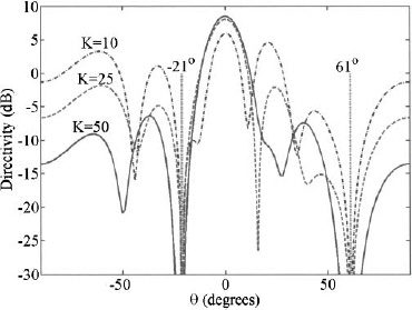
Figure 8.23. The SMI adapted pattern after K = 10,25, and 50 samples.

8.4.2.4. Recursive Least Squares Algorithm. The recursive least squares (RLS) algorithm recursively updates the correlation matrix such that more recent time samples receive a higher weighting than past samples [31]. A straightforward implementation of the algorithm is written as

and the correlation vector is

where the forgetting factor, α, is limited by 0 ≤ α ≤ 1. Higher values of α give more weight to previous values than do lower values of α. An even better relationship calculates an update for the inverse of the correlation matrix [31]

with the weights given by

Example. An 8-element uniform array with λ/2 spacing has the desired signal incident at 0° and two interference signals incident at −21° and 61°. Use the RLS algorithm to place nulls in the antenna pattern. Assume σ_n = 0.01. The signal is represented by (8.11) and the interference by (8.9).

Figure 8.24. The adapted pattern after the RLS algorithm ran for 25 iterations. The signal is at 0° and the interference is at −21° and 61°.

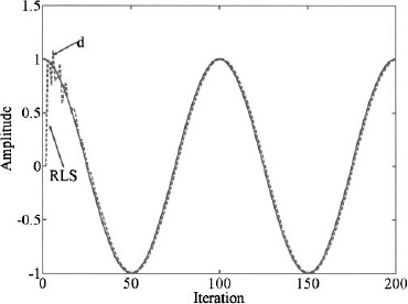
Figure 8.25. The RLS signal (dashed line) and the actual signal (solid line).

After K = 25 iterations and α = 0.9, the antenna pattern appears in Figure 8.24 with a directivity of 8.6 dB. Figure 8.25 shows the RMS signal superimposed on the real signal as a function of iteration. Figure 8.26 and Figure 8.27 are the RMS weights. They converge in about 15 iterations.

Figure 8.26. The amplitude weights versus iteration for the RMS algorithm.

Figure 8.27. The phase weights versus iteration for the RMS algorithm.

8.4.2.5. Comparing the LMS, SMI, and RLS Algorithms. The LMS algorithm slowly converges when the ratio of the maximum to minimum eigenvalue of the correlation matrix is large. A large eigenvalue ratio implies that there are narrow valleys in the cost surface [33], so the method of steepest descent converges slowly. Since the amplitude of the eigenvalues of the correlation matrix are proportional to the interference signal powers, the LMS algorithm converges fast when the interference powers are similar and slow when they are not. Figure 8.28 shows the adapted pattern after 1000 iterations with a null placed at 21° but not at −21°. The 0-dB desired signal was incident on the 8-element array at 0°, while a −10-dB interference was incident at 21° and a 0dB interference was incident at −21°.

Figure 8.28. The adapted array factor for the LMS algorithm after K = 1000 iterations when a 0-dB signal is incident at 0°, and a −10-dB interference is incident at −21° and a 0-dB interference is incident at 21°.

Figure 8.29. Plot of the RLS signal (100 iterations) versus the LMS signal as a function of iteration when a 0-dB signal is incident at 0° and a −12-dB interference is incident at −21° and 61°.

Figure 8.29 is a plot of the received signal as a function of iteration for the RLS and LMS algorithms when the 0-dB desired signal was incident on the 8-element array at 0° while 12−dB interference signals are incident at −21° and 61°. Note that the RLS algorithm converges within a few iterations, while the LMS takes many iterations. The forgetting factor plays an important role in speeding convergence.

Figure 8.30. Plot of the received signal for the RLS and LMS algorithms when the noise is σ_noise = 0.1.

The algorithms are also sensitive to noise. Increasing the noise from σ_noise = 0.01 to σ_noise = 0.1 significantly reduces the effectiveness of the adaptive algorithms. Figure 8.30 is a plot of the received signal recovered by the LMS and RLS algorithms. The LMS is much more sensitive to noise than the RLS algorithm. Figure 8.31 shows the adapted patterns after 100 iterations. The RLS algorithm places deep nulls at –21° and 61°, while the SMI algorithm has a null at 61° but a small sidelobe at –21°. On the other hand, the LMS algorithm has a null at –21° but a sidelobe still remains at 61°.

8.4.3. Adaptive Nulling via Power Minimization

Another class of adaptive nulling algorithms adjusts the array weights until the total output power is minimized. These algorithms are cheap to implement, because they use the existing array architecture without expensive additions, such as digital beam forming. Since a digital beamformer is not needed, array calibration is simpler too. Their drawbacks include slow convergence and possibly high pattern distortions. This approach only works if the desired signal is not present or if the gain of the cancellation beams in the adaptive algorithm is small compared to the main beam gain. Sidelobe cancelers are an example of limiting the nulling to the sidelobes, because the gain of the auxiliary antennas are too small to have a major impact on the main beam, but large enough to cancel sidelobes.

Figure 8.31. Adapted array factors for the SMI, RLS, and LMS algorithms after K = 50, 200, and 1000 iterations when a 0-dB signal is incident at 0° and a –12-dB interference is incident at –21° and 61°.

Making only a few of the array elements adaptive prevents the destruction of the main beam but allows nulls to be placed in the sidelobes [35]. Enough elements are selected to place a null in the highest sidelobe without significantly distorting the main beam. A second approach forms an approximate numerical gradient and uses a steepest descent algorithm to find the minimum output power [36]. As long as the weight changes are small and the sidelobes are low, little main beam distortion occurs while placing the nulls. This approach has been implemented experimentally but is slow and can get trapped in a local minimum. As a result, the best weight settings to achieve appropriate nulls are usually not found. A final approach limits the array weight settings. Large reductions in the amplitude weights are required in order to reduce the main beam. Consequently, if only small amplitude and phase perturbations are allowed, then a null cannot be placed in the main beam but can be placed in the sidelobes. Lower sidelobes require smaller perturbations to the weights in order to place the null. Using only a few least significant bits of the digital phase shifter and attenuator prevents the algorithm from placing nulls in the main beam. The amplitude and phase associated with each bit of a digital weight (up to 8 bits) is shown in Table 8.5. The lower bits are quite capable of disrupting the main beam. For instance, giving half the elements a 180° phase shift (bit 1) will place a null in the peak of the main beam.

Example. A 20-element, 20-dB, = 3 Taylor linear array with elements spaced half a wavelength apart has 6-bit amplitude and phase weights. If the only source enters the main beam, then the adaptive algorithm tries to reduce the main beam in order to reduce the total output power. Show how using 1 through 4 least significant bits (bits 3 to 6) alters the main beam.

TABLE 8.5. Amplitude and Phase Values of the Nulling Bits when There Are a Total of 6 bits for the Amplitude and Phase Weights

Figure 8.32. Maximum main beam reduction possible when 1 to 4 least significant bits out of 6 total bits in an amplitude weight are used to null a signal at = 90°. 0 bits is the quiescent pattern.

Figure 8.32 (amplitude weights) and Figure 8.33 (phase weights) show the main beam reduction when the following bits from Table 8.5 are used:

1. bit 6
2. bits 5,6
3. bits 4,5,6
4. bits 3,4,5,6

Figure 8.33. Maximum main beam reduction possible when 1 to 4 least significant bits out of 6 total bits in a phase weight are used to null a signal at = 90°. 0 bits is the quiescent pattern.

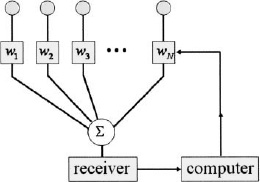
Figure 8.34. Diagram of an adaptive antenna that minimizes the total output power.

A maximum reduction of 1 dB is possible using four least significant bits of amplitude. Using one through three least significant bits results in very little perturbation to the main beam. Unlike amplitude-only nulling, phase-only nulling causes beam squint. The phase had more effect on the main beam than did amplitude. This example demonstrates that adaptive nulling with the least significant bits would not result in significant degradation to the main beam.

A diagram of the adaptive array appears in Figure 8.34. The array has a corporate feed with variable weights at each element. The phase shifters in the weights are available for beam steering and calibration as well as nulling. The amplitude weights are used for low-sidelobe tapers and calibration. This adaptive array configuration is much simpler and cheaper than the digital beamforming array required by other adaptive algorithms.

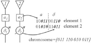
Figure 8.35. The least significant bits of the amplitude phase weights are put in a chromosome.

Figure 8.36. Two parents are selected from the mating pool. Two offspring are created using single-point crossover and placed into the population matrix to replace discarded chromosomes.

8.4.3.1. Amplitude and Phase Adaptive Nulling. To demonstrate the concept of adaptive nulling through power minimization, consider an array with 5-bit amplitude and phase weights at each element. To prevent main beam nulling and severe pattern distortion, the genetic algorithm that performs the adaptive nulling controls only the 3 least significant bits of each weight. A vector called a chromosome stores the adaptive bits as shown in Figure 8.35. All the chromosomes under consideration make up the N_pop rows of the population matrix. In this case, there are 3 bits/weight, 2 weights per element, and N_adap adaptive elements in the array, so the population matrix is N_pop × 6N_adap. Each chromosome in the population is then sent from the computer to the antenna to adjust the weights, and the output power is measured and stored as the cost associated with the chromosome (Figure 8.37). Low-cost chromosomes become parents and mate to form offspring as shown in Figure 8.36 (single point crossover used here). Mutations occur inside the population (italicized digits in Figure 8.37). This process continually adjusts the antenna pattern by placing nulls in the sidelobes while having minimal impact on the main beam as shown in Figure 8.38.

Figure 8.37. Random bits in the population are mutated (italicized bits). The chromosomes are sent to the array one at a time and the total output power measured. Each chromosome then has an associated output power.

Figure 8.38. Flow chart of the adaptive genetic algorithm with a linear array.

Figure 8.39. Signal levels as a function of generation for the phase-only algorithm.

Example. A 20-element array of point sources spaced 0.5λ apart has 6-bit amplitude and phase weights and a 20-dB, = 3, low-sidelobe Taylor amplitude taper. The desired signal is incident on the peak of the main beam and is normalized to one or 0dB. Two 30-dB jammers enter the sidelobes at 111° and 117°. The genetic algorithm has a population size of 8 and a mutation rate of 10%.

Figure 8.39 are the power levels received by the array. The total power level decreases while the desired signal power remains relatively constant. Sometimes, one jammer power goes down while the other jammer power goes up. The ratio of the signal power to the jammer power is graphed in Figure 8.40. Figure 8.41 shows the adapted antenna pattern superimposed on the quiescent pattern.

Amplitude- and phase-adaptive nulling with a genetic algorithm was experimentally demonstrated on a phased array antenna developed by the Air Force Research Laboratory (AFRL) at Hanscom AFB, MA [37]. The antenna has 128 vertical columns with 16 dipoles per column equally spaced around a cylinder that is 104cm in diameter (Figure 8.42). Figure 8.43 is a cross-sectional view of the antenna. Summing the outputs from the 16 dipoles forms a fixed elevation main beam pointing 3° above horizontal. Only eight columns of elements are active at a time. Consecutive eight-elements form a 22.5° arc (1/16 of the cylinder), with the elements spaced 0.42λ apart at 5 GHz. Each element has an 8-bit phase shifter and 8-bit attenuator. The phase shifters have a least significant bit equal to 0.0078125π radians. The attenuators have an 80-dB range with the least significant bit equal to. 3125 dB. The antenna has a quiescent pattern resulting from a 25-dB, = 3 Taylor amplitude taper. Phase shifters compensate for the curvature of the array and unequal path lengths through the feed network.

Figure 8.40. The signal-to-interference ratio for the phase-only adaptive algorithm with two jammers at 111° and 117°.

Figure 8.41. Adapted pattern for phase-only nulling with two jammers.

A 5-GHz continuous-wave source served as the interference. Only the four least significant bits of the phase shifters and attenuators were used. The genetic algorithm had a population size of 16 chromosomes and used single point crossover. Only one bit in the population was mutated every generation, resulting in a mutation rate of 0.1%. Nulling tended to be very fast with the algorithm placing a null down to the noise floor of the receiver in less than 30 power measurements. Two cases of placing a single null are presented here. The first example has the interference entering the sidelobe at 28°, and the second example has the interference at 45°. Figure 8.44 plots the sidelobe level at 28° and 45° as a function of generation. The resulting far-field pattern measurements are shown in Figures 8.45 and 8.46 superimposed on the quiescent pattern. These examples demonstrate that the genetic algorithm quickly places nulls in the sidelobes in the directions of the interfering signals by minimizing the total power output.

Figure 8.42. Experimental adaptive cylindrical array (R. L. Haupt, Adaptive nulling with a cylindrical array, AFRL-SN-RS-TR-1999-36, March 1999).

Figure 8.43. The cylindrical array has 128 elements, with 8 active at a time.

Figure 8.44. Convergence of genetic algorithm for jammers at 28° and 45°.

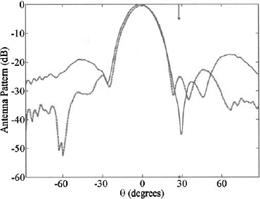
Figure 8.45. Null placed in the far-field pattern at 28°.

Figure 8.46. Null placed in far-field pattern at 45°.

Figure 8.47. Photograph of 8-element adaptive array (courtesy of Andrea Massa, University of Trento).

The particle swarm optimization algorithm has also been used for adaptive nulling [38]. As an example, the 2.4-GHz 8-element array of eight equally spaced (d = λ/2) dipole elements above a ground plane is shown in Figure 8.47 served as an adaptive antenna with amplitude and phase weights at each element. A passive RF power combiner with seven microstrip Wilkinson power combiners sent the output power to a spectrum analyzer in order to estimate the SINR (signal-to-interference-plus-noise ratio). The particle swarm algorithm adjusted the weights through a vector modulator in order to maximize the SINR. Figure 8.48 shows plots of the computed and measured adapted antenna patterns.

8.4.3.2. Phase-Only Adaptive Nulling. A phased array may or may not have variable amplitude weights but always has phase shifters for beam steering and calibration. Since the phase weights already exist, why not use the phase shifters as adaptive weights? The theory behind phase-only nulling first appeared in reference 39. The authors present a beam-space algorithm derived for a low-sidelobe array and assume that the phase shifts are small. When the direction of arrival for all the interfering sources is known, then cancellation beams in the directions of the sources are subtracted from the original pattern. Adaptation consists of matching the peak of the cancellation beam with the culprit sidelobe and subtracting [40].

Figure 8.48. Computed and measured adapted antenna patterns (courtesy of Andrea Massa, University of Trento).

The new phase settings that minimize the output power can be found by using the method of steepest descent [25].

where P(κ) is the array output power at time step κ, δ_n(κ) is the phase shift at element n, Δ(κ) is the small phase increment, and

This algorithm was tested for phase-only simultaneous nulling of the sum and difference patterns of an 80-element linear array of H-plane sectoral horns [25]. The sum channel had a 30-dB Taylor taper, and the difference channel had a 30-dB Bayliss taper. Both channels shared the 8-bit beam steering phase shifters. No source was present in the main beam, but one CW source was aimed at the sidelobes in the quiescent sum and difference patterns at 23°. If the algorithm is only used to minimize the sum channel output, then the resulting sum pattern appears in Figure 8.49 with the difference pattern in Figure 8.50. A null appears in the sum pattern but not the difference pattern. Minimizing the output from both channels results in the patterns shown in Figures 8.51 and 8.52. This time, nulls are placed in both patterns.

Figure 8.49. Sum patterns due to adaptive nulling in the sum pattern only.

Figure 8.50. Difference patterns due to adaptive nulling in the sum pattern only.

Figure 8.51. Sum patterns due to simultaneous adaptive nulling in the sum and difference patterns.

Figure 8.52. Difference patterns due to simultaneous adaptive nulling in the sum and difference patterns.

The gradient method is slow, because the phase at each element is serially toggled for a power measurement every iteration. Also, the steepest descent algorithm can get stuck in a local minimum. A genetic algorithm was first proposed for phase-only adaptive nulling in reference 41.

Figure 8.53. Convergence of the phase-only adaptive nulling algorithm using a genetic algorithm.

Figure 8.54. Signal-to-jammer ratio versus generation of the phase-only adaptive nulling algorithm using a genetic algorithm.

Example. A 20-element array of point sources spaced 0.5λ apart has 6-bit phase shifters and a 20-dB, = 3 low-sidelobe Taylor amplitude taper. The desired signal is incident on the peak of the main beam and is normalized to one or 0dB. Two 30-dB jammers enter the sidelobes at 111° and 117°. The genetic algorithm has a population size of 8 and a mutation rate of 10%.

The algorithm successfully placed nulls at both angles. The convergence is shown in Figure 8.53 while the increasing signal to jammer ratio appears in Figure 8.54. Figure 8.55 shows the adapted pattern compared to the quiescent pattern.

Figure 8.55. Adapted array pattern for phase-only adaptive nulling algorithm using a genetic algorithm.

Figure 8.56. Convergence of the phase-only algorithm with symmetric jammers.

Moving to the case of two 30-dB interference sources at 50° and 130° confronts the adaptive algorithm with the problem of symmetric interference sources. The genetic algorithm could only null one of the interference sources with three least significant phase bits, so a minimum of four had to be used. Adding a fourth bit resulted in nice convergence as shown in Figure 8.56. As noted previously, four phase bits results in noticeable main lobe degradation as shown in Figure 8.57.

Figure 8.57. Adapted pattern for phase-only nulling with symmetric jammers.

Phase-only nulling has the advantage of simple implementation. The tradeoff is that more bits must be used to null interference signals that are at symmetric locations about the main beam. The additional nulling bits result in higher distortions in the main beam and sidelobes. Small phase shifts produce symmetric cancellation beams that are 180° out of phase. When they are added to the quiescent pattern to produce a null at one location, the symmetric sidelobe increases. Allowing larger phase shifts [42] or adding amplitude control overcomes this problem.

8.4.3.3. Amplitude-Only Adaptive Nulling. Although not very common, an array can have variable amplitude weights at the elements without phase shifters. Vu suggested moving conjugate zeros on the unit circle in the direction of interfering sources [43]. This approach is not adaptive and depends upon the ability of finding the locations of the interfering sources. All the zeros that are not used to place nulls can then be used to control the rest of the array factor.

The simulated array consists of eight vertically polarized dipoles spaced 0.075λ with a variable amplitude weight at the two elements on each end of the array. It is a narrow band system operating at 2 GHz. Two signals are incident upon the array. A 0-dB desired signal appears at = 90° and an undesired signal appears at = 68°. The GA found the amplitude settings for the four dipoles as appears in Table 8.6. The three-dimensional quiescent and adapted patterns are shown in Figure 8.58. Table 8.7 indicates that the gain decreases by 1.2 dB while the sidelobe in the direction of the interference decreases by 19.2 dB. As a result, the signal-to-noise ratio (SNR) increases from –4.2 dB to 31.9 dB. Pattern cuts for the quiescent and adapted arrays are shown in Figure 8.59.

TABLE 8.6. The Quiescent and Adapted Amplitude Weights for the 8-Element Array

Figure 8.58. (a) Quiescent and (b) adapted patterns for the 8-element amplitude-only dipole array.

TABLE 8.7. Array Pattern Statistics for the Quiescent and Adapted Arrays

A 2.2-GHz, 8-element array was made from monopole/switch elements as shown in Figure 8.60. The elements have a variable switch controlled by an IR LED [44]. The corporate feed consists of 8 low-loss, phase-stable coaxial cables and a broadband 8-to-1 power combiner. Only the two edge elements on either side of the array are used by a genetic algorithm to place nulls. The measured S₁₁ of the array is below −10 dB from 2.11 to 2.53 GHz for a bandwidth of 18.4%. Figures 8.61 and 8.62 are the measured amplitude and phase of S₁₂ for the adaptive elements in the array (the numbers on the plots correspond to the element numbers in Figure 8.60) as a function of LED current.

Figure 8.63 shows the adapted pattern superimposed on the quiescent pattern when only a 10-dBm signal at –35° is present. The main beam loses 3.9 dB while the null is 42dB below the sidelobe at –35°. A second example shows the results of placing two signals of 15dBm at –19° and –35° (Figure 8.64). No signal is incident upon the main beam. In this case, the main beam is reduced by 3.6 dB. The sidelobe at –19° goes down 13 dB, and the sidelobe at –35° is reduced by 9dB.

Figure 8.59. Quiescent and adapted pattern cuts.

Figure 8.60. Experimental linear array of broadband monopole elements with variable IR switches for amplitude control.

Figure 8.61. Measured S₂₁ of the elements as a function of diode current.

Figure 8.62. Measured phase of S₁₂ of the elements as a function of diode current.

8.5. MULTIPLE-INPUT MULTIPLE-OUTPUT (MIMO) SYSTEM

A typical communications system has one antenna for transmit and one antenna for receive, which is known as a single-input single-output system. Another version has a single antenna on transmit and an array on receive. This version is known as single input and multiple output. The converse of an array on transmit with a single antenna on receive is a multiple input single output system. These types of systems have driven the need for antenna arrays for many years.

Figure 8.63. Adapted and quiescent far-field patterns when a signal is incident at –35°.

Figure 8.64. Adapted and quiescent far-field patterns when a signal is incident at –19° and –35°.

A multiple-input multiple-output (MIMO) system uses an array for transmit as well as another array for receive (Figure 8.65). As a result, both antennas can be smart or adaptive to increase the amount of data transferred over the communications channel. MIMO was developed to counteract the problems associated with multipath in wireless communications. A MIMO system increases its capacity in rich multipath environments by exploiting the spatial properties of the multipath channel, thereby offering an additional dimension that enhances communication performance. A beam is synthesized to transmit data to a single user while placing nulls in the directions of the other users. An array provides antenna or spatial diversity, because more than one element transmits/receives the same signal from different locations. Separating the antenna elements causes the signals from M transmitting antennas to take different paths to the N receiving antennas. The received signals are a function of the transmitted signals, the channel paths, and the noise [45].

Figure 8.65. Signal paths between transmit and receive antennas in a MIMO system.

where is the noise vector and H is the channel matrix given by

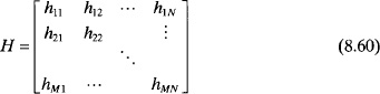
and the channel matrix elements, h_mn, are the transfer functions describing the channel between transmit antenna m and receive antenna n. In order to recover the transmitted data, s, an accurate estimate of H is needed. The transmitted data are then calculated from the received data by inverting the channel matrix

If the medium were free space, then these channel matrix elements would just be the free-space Green’s function and H is written as

Multipath, noise, fading, Doppler shift, coupling, and interference all contribute to variations in the H matrix that are difficult to analytically or numerically predict. Consequently, H is usually found through experimentation.

The power received by the array is given by

The M × M matrix HH^† can be decomposed as

The singular value decomposition of H is given by [46]

where

= singular values

U_SVD, V_SVD = singular vectors

The singular values are just the square root of the eigenvalues in (8.64). Substituting (8.65) into (8.59) results in

This equation can be written as

Figure 8.66. Condition number of H as a function of element spacing.

where

There are g parallel independent radio subchannels between the transmit and receive antennas, where g is the rank of H. The rank of a matrix is the number of nonzero singular values.

Example. A MIMO system has a 3-element array of isotropic point sources spaced d apart on transmit and receive. The system operates at 2.4 GHz and the arrays are 100 m apart and face each other. Show how the condition number of H changes as the element spacing increases.

Figure 8.66 shows how the condition number of H decreases as the element spacing for both the transmit and receive arrays increase. Increasing the element spacing in only the transmit or receive array also decreases the condition number but not as fast. The lower the condition number, the more accurate the inversion of H is.

8.6. RECONFIGURABLE ARRAYS

A reconfigurable array changes its performance characteristics by using switches, such as MEMS or PIN diodes, to connect elements to adjacent structures. The 5-element array in Figure 8.67 has elements that are rectangular patches made from a PEC that is 58.7 × 39.4 mm. The substrate is a slab of optically transparent fused quartz with ε_r = 3.78 backed by a PEC ground-plane. The substrate is 88.7 × 69.4 mm and is 3 mm thick. The patch has a thin strip of silicon (G) 58.7 × 2mm with ε, = 11.7. The right edge of the patch is a thin strip of PEC (F) 58.7 × 4.2 mm. A laser or LED beneath the groundplane illuminates the silicon through small holes in the groundplane or by making the groundplane from a transparent conductor. The silicon conductivity is a function of the light intensity. A graph of the amplitude of the return loss is shown in Figure 8.68 for the following conductivities: 0, 2, 5, 10, 20, 50, 100, 200, and 1000 S/m. At 2 GHz, there is a distinct resonance when the silicon has no conductivity. As the conductivity increases, the resonance is at 1.78 GHz. The amount of power delivered to the patch at 2 GHz reduces as the conductivity increases, so the photoconductive silicon acts as an amplitude control to that element.

Figure 8.67. Diagram of the adaptive reconfigurable patch array.

The element spacing is 75 mm or 0.5λ. If the silicon insets all have a conductivity of zero, then the array is uniform with a far-field pattern shown in Figure 8.69. This quiescent pattern has a gain of 12.81 dB and a relative peak sidelobe level of 13.84 dB. The element patterns of the uniform array are shown in Figure 8.70. The average gain of these patterns at boresight is 6.14 dB.

Increasing the conductivity of the silicon in a patch decreases the product of the patch gain times the power delivered to the patch. Carefully tapering the illumination of the LEDs creates an amplitude taper. An array pattern with equal sidelobes results when the conductivity has values of [16 5 0 5 16] S/m (Figure 8.69). The antenna pattern has a gain of 10.4 dB with a peak relative sidelobe level of 23.6 dB. The upper-left element patterns correspond to the uniform array. Applying the illumination taper produces the element patterns shown in Figure 8.70.

Figure 8.68. Plots of the magnitude of s₁₁ for silicon conductivities of 0,2,5,10,20,50, 100, 200, and 1000 S/m.

Figure 8.69. The quiescent pattern is the dashed line and has all the conductivities set to 0. The adapted pattern is the solid line and has the silicon conductivities set to [16 5 0 5 16] S/m.

The antenna in Figure 8.71 has a Z-shaped active microstrip element in the center of 18 identical, equally spaced parasitic metallic elements. Its operating frequency is 2.45 GHz. The parasitic elements have PIN diodes (activated elements in black and deactivated elements in gray color) that connect adjacent elements. Connecting several adjacent parasitic elements steers the main lobe in azimuth. The beamwidth depends upon the number of parasitic elements connected together. The dark parasitic elements in Figure 8.71 correspond to the ones that are connected by the PIN diodes. Plots of the computed and measured far-field patterns are also shown in Figure 8.71.

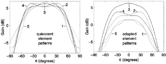
Figure 8.70. The element patterns of the array that has the silicon conductivities set to [16 5 0 5 16] S/m.

Figure 8.71. Adaptive antenna that uses parasitic elements.

Figure 8.72. Plot of the percent element failures required to raise the average sidelobe level of an 8000 element circular array with a 40-dB Taylor amplitude taper and triangular element spacing with d = 0.5λ by 3 or 6dB for several cluster sizes.

As noted in Chapter 2, element failures reduce gain and increase sidelobe levels. At some point, the failures cause the system to shut down. To develop an acceptable maintenance schedule and to reduce the probability of a catastrophic array failure, the mean time between failure of the array should be maximized by minimizing the component failure rate and selecting an appropriate array architecture.

The cost of an array consists of the production cost (design, purchase and/or fabrication of parts, assembly, and testing of the antenna) and the life-cycle cost (cost over an antenna’s operational lifetime to replace or repair all failed components in the antenna). The life-cycle cost is highly dependent upon the component MTBF. Usually, the array has a very high passive component MTBF, so its contribution to the life-cycle cost is ignored here. On the other hand, the MTBF of active components, such as T/R modules and power supplies, drive the life-cycle cost of an antenna.

Performance degredation is defined in terms of increased peak and/or average sidelobes from associated with the component failures. If one T/R module feeds multiple elements, then the T/R module failure results in a cluster of element failing. The larger the cluster, the more devastating the failure is. Figure 8.72 is a plot of the percent element failures required to raise the average sidelobe level by 3 or 6dB for several cluster sizes for an 8000-element circular array with a 40-dB Taylor amplitude taper and triangular element spacing with d = 0.5λ [47]. Using components with high MTBF, reducing the number of elements, and adding redundancy increases the array MTBF.

In order to reduce the effects of element failures, the element weights can be recalculated to bring the sidelobe levels down. Techniques for finding these new element weights are described in reference 48 for corporate arrays and for digital beamforming arrays [49]. Recently, more sophisticated approaches using a genetic algorithm [50] and an iterative method using the inverse Fourier transform [51]. In all cases, the location of the failed elements must be known to calculate the weight corrections.

REFERENCES

1. L. C. V. Atta, Electromagnetic Reflector, 2,908,002, U.S.P. Office, 1959.
2. S. Drabowitch, Modern Antennas, 2nd ed., Dordrecht: Springer, 2005.
3. M. Skolnik and D. King, Self-phasing array antennas, IEEE Trans. Antennas and Propagat., Vol. 12, No. 2, 1964, pp. 142–149.
4. C. Pon, Retrodirective array using the heterodyne technique, IEEE Trans. Antennas and Propagat., Vol. 12, No. 2, 1964, pp. 176–180.
5. R. Y. Miyamoto and T. Itoh, Retrodirective arrays for wireless communications, IEEE Microwave Mag, Vol. 3, No. 1, 2002, pp. 71–79.
6. S. Lim and T. Itoh, A 60 GHz retrodirective array system with efficient power management for wireless multimedia sensor server applications, IET Microwaves Antennas Propagat, Vol. 2, No. 6, 2008, pp. 615–625.
7. T. Y. Y. L. Chiu, W. S. Chang, Q. Xue, C. H. Chan, Retrodirective array for RFID and microwave tracking beacon applications, Microwave Opt. Technol. Lett., Vol. 48, No. 2, 2006, pp. 409–411.
8. B. Nair and V. F. Fusco, Two-dimensional planar passive retrodirective array, Electron. Lett., Vol. 39, No. 10, 2003, pp. 768–769.
9. M. K. Watanabe, R. N. Pang, B. O. Takase et al., A 2-D phase-detecting/heterodyne-scanning retrodirective array, IEEE Trans. Microwave Theory Tech., Vol. 55, No. 12, 2007, pp. 2856–2864.
10. R. Compton, Jr., On eigenvalues, SINR, and element patterns in adaptive arrays, IEEE Trans. Antennas Propagat., Vol. 32, No. 6, 1984, pp. 643–647.
11. A. W. Rudge, The Handbook of Antenna Design, 2nd ed., London: P. Peregrinus on behalf of the Institution of Electrical Engineers, 1986.
12. S. Chandran, Advances in Direction-of-Arrival Estimation, Boston: Artech House, 2006.
13. J. Capon, High-resolution frequency-wavenumber spectrum analysis, Proc. IEEE, Vol. 57, No. 8, 1969, pp. 1408–1418.
14. R. Schmidt, Multiple emitter location and signal parameter estimation, IEEE Trans. Antennas and Propagat., Vol. 34, No. 3, 1986, pp. 276–280.
15. R. Schmidt and R. Franks, Multiple source DF signal processing: An experimental system, IEEE Trans. Antennas Propagat, Vol. 34, No. 3, 1986, pp. 281–290.
16. A. Barabell, Improving the resolution performance of eigenstructure-based direction-finding algorithms, IEEE International Conference on Acoustics, Speech, and Signal Processing, 1983, pp. 336–339.
17. J. P. Burg, The relationship between maximum entropy spectra and maximum likelihood spectra, Geophysics, Vol. 37, No. 2, 1972, pp. 375–376.
18. R. T. Lacoss, Data adaptive spectral analysis methods, Geophysics, Vol. 36, No. 4, 1971, pp. 661–675.
19. V. F. Pisarenko, The retrieval of harmonics from a covariance function, Geophys. J. Int., Vol. 33, No. 3, 1973, pp. 347–366.
20. A. Paulraj, R. Roy, and T. Kailath, A subspace rotation approach to signal parameter estimation, Proc. IEEE, Vol. 74, No. 7, 1986, pp. 1044–1046.
21. L. C. Godara, Smart Antennas, Boca Raton, FL, CRC Press, 2004.
22. P. Howells, Explorations in fixed and adaptive resolution at GE and SURC, IEEE Trans. Antennas Propagat., Vol. 24, No. 5, 1976, pp. 575–584.
23. B. Widrow, P. E. Mantey, and L. J. Griffiths et al., Adaptive antenna systems, Proc. IEEE, Vol. 55, No. 12, 1967, pp. 2143–2159.
24. R. A. Monzingo, T. W. Miller, and Knovel (Firm), Introduction to Adaptive Arrays, Scitech, 2004.
25. R. L. Haupt, Adaptive nulling in monopulse antennas, IEEE Trans. Antennas Propagat., Vol. 36, No. 2, 1988, pp. 202–208.
26. R. L. Haupt and D. H. Werner, Genetic Algorithms in Electromagnetics, Hoboken, NJ: IEEE Press/Wiley-Interscience, 2007.
27. M. I. Skolnik, Radar Handbook, New York: McGraw-Hill, 2007.
28. H. M. Finn, R. S. Johnson, and P. Z. Peebles, Fluctuating target detection in clutter using sidelobe blanking logic, Aerospace and Electronic Systems, IEEE Transactions on, Vol. AES-7, No. 1, 1971, pp. 147–159.
29. A. Farina, Single sidelobe canceller: theory and evaluation, IEEE Trans. Aerosp. Electron. SySt., Vol. AES-13, No. 6, 1977, pp. 690–699.
30. S. Applebaum, Adaptive arrays, IEEE Trans. Antennas and Propagat, Vol. 24, No. 5, 1976, pp. 585–598.
31. F. B. Gross, Smart Antennas for Wireless Communications: With MATLAB, New York: McGraw-Hill, 2005.
32. R. T. Compton, Adaptive Antennas: Concepts and Performance, Philadelphia: Prentice-Hall, 1987.
33. W. H. Press and Numerical Recipes Software (Firm), Numerical recipes in FORTRAN, Cambridge University Press, 1994.
34. I. Gupta, SMI adaptive antenna arrays for weak interfering signals, IEEE Trans. Antennas and Propagat, Vol. 34, No. 10, 1986, pp. 1237–1242.
35. D. Morgan, Partially adaptive array techniques, IEEE Trans. Antennas and Propagat, Vol. 26, No. 6, 1978, pp. 823–833.
36. R. Haupt, Adaptive nulling in monopulse antennas, IEEE Trans. Antennas and Propagat., Vol. 36, No. 2, 1988, pp. 202–208.
37. R. L. Haupt and H. Southall, Experimental adaptive cylindrical array, Microwave Journal, 1999, pp. 291–296.
38. M. Benedetti, R. Azaro, and A. Massa, Experimental validation of fully-adaptive smart antenna prototype, Electron. Lett., Vol. 44, No. 11, 2008, pp. 661–662.
39. C. Baird and G. Rassweiler, Adaptive sidelobe nulling using digitally controlled phase-shifters, IEEE Trans. Antennas Propagat., Vol. 24, No. 5, 1976, pp. 638–649.
40. H. Steyskal, Simple method for pattern nulling by phase perturbation, IEEE Trans. Antennas and Propagat., Vol. 31, No. 1, 1983, pp. 163–166.
41. R. L. Haupt, Phase-only adaptive nulling with a genetic algorithm, IEEE Trans. Antennas Propagat., Vol. 45, No. 6, 1997, pp. 1009–1015.
42. R. Shore, Nulling a symmetric pattern location with phase-only weight control, IEEE Trans. Antennas and Propagat., Vol. 32, No. 5, 1984, pp. 530–533.
43. T. B. Vu, Method of null steering without using phase shifters, IEE Proc. Microwaves Opt. Antennas, H, Vol. 131, No. 4, 1984, pp. 242–245.
44. J. R. Flemish, H. W. Kwan, R. L. Haupt et al., A new silicon-based photoconductive microwave switch, Microwave Optical. Technol. Lett., IEEE Aerospace Conference, Vol. 51, No. 1, 2009, pp. 248–252.
45. S. M. Alamouti, A simple transmit diversity technique for wireless communications, IEEE J. Selected Areas Commun., Vol. 16, No. 8, 1998, pp. 1451–1458.
46. M. A. Jensen and J. W. Wallace, A review of antennas and propagation for MIMO wireless communications, IEEE Trans. Antennas Propagat., Vol. 52, No. 11, 2004, pp. 2810–2824.
47. A. K. Agrawal and E. L. Holzman, Active phased array design for high reliability, IEEE Trans. Aerosp. Electron. Syst., Vol. 35, No. 4, 1999, pp. 1204–1211.
48. T. J. Peters, A conjugate gradient-based algorithm to minimize the sidelobe level of planar arrays with element failures, IEEE Trans. Antennas and Propagat., Vol. 39, No. 10, 1991, pp. 1497–1504.
49. R. J. Mailloux, Phased array error correction scheme, Electron. Lett., Vol. 29, No. 7, 1993, pp. 573–574.
50. S. Seong Ho, S. Y. Eom, S. I. Jeon et al., Automatic phase correction of phased array antennas by a genetic algorithm, IEEE Trans. Antennas Propagat, Vol. 56, No. 8, 2008, pp. 2751–2754.
51. W. P. N. Keizer, Element Failure Correction for a large monopulse phased array antenna with active amplitude weighting, IEEE Trans. Antennas and Propagat., Vol. 55, No. 8, 2007, pp. 2211–2218.