2Array Factor Analysis

This chapter presents the fundamental approaches to the analysis of linear and planar arrays of point sources. Element patterns, polarization, and mutual coupling are delayed until future chapters. Keeping the elements along a straight line or in a plane are the most common array configurations. Other types of nonplanar arrays will be discussed in future chapters.

2.1. THE ARRAY FACTOR

A single isotropic point source transmits a field as derived in Chapter 1. If that point source transmits to an array of point sources, then the output of the array is proportional to the weighted sum of the received signal from each element in the array.

where R_n = distance from element n to the point at (x_f, y_f z_f). As shown in Chapter 1, the phase of the received signal at the element is positive, because the signal is traveling toward the element. A transmit array has a minus sign in the phase, because the radiation is going away from the antenna. Figure 2.1 is a diagram of a point source transmitting to an array of point sources. When the array is very far from the point source, then all the R_n in the denominator of (2.1) are approximately the same. Consequently, the field is proportional to the sum of the weighted phase factors.

Most arrays are either linear or planar. A linear array has all of its elements lying along a straight line. To make calculations easy, assume that the array lies along the x, y, or z axes. The phase reference, or point of zero phase, is chosen to be either the first element or the physical center of the array. The origin of the coordinate system is placed at the phase center. An incident plane wave arrives at all of the elements at the same time when the incident field is normal or broadside to the array. When the plane wave is off-normal, then the plane wave arrives at each element at a different time. Thus, the phase difference between the signals received by the elements is accounted for by an appropriate phase delay before summing the signals to get the array output. An example of the phase difference between two elements along the x axis is shown in Figure 2.2. If the incident wave vector is in the x−y plane, then the phase is a function of . If the incident wave vector is in the x−z plane, then the phase is a function of θ. The array factor or antenna pattern due to isotropic point sources is a weighted sum of the signals received by the elements.

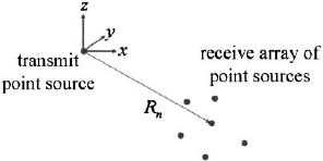
Figure 2.1. Near field of the array.

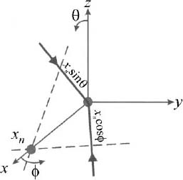
Figure 2.2. Phase difference between two elements on the x axis. The dashed line is the plane wave, and the arrows indicate the direction of propagation.

where N is the number of elements, w_n = a_ne^jδn is the complex weight for element n, k = 2π/λ, (x_n, y_n, z_n) is the location of element n, (θ,) is the direction in space, and

Equations (2.2) and (2.3) are the same when ψ_n = kR_n. The definition of the variable, u, depends upon which plane contains the array and the incident field vector. In digital signal processing terms, this equation is a spatial finite impulse response (FIR) filter. The diagram of a linear array in Figure 2.3 shows the signals sampled at discrete points in space/time and then weighted and summed.

A planar array has all of its elements in the same plane. By convention, the elements of a planar array usually lie in the x−y plane with the z axis pointing away from broadside. Thus, θ is measured from broadside and is often called the elevation angle, while is measured from the x axis and is often called the azimuth angle. Figure 2.4 is a diagram of a planar array with elements lying in arbitrary positions in the x−y plane. Of course, the array can lie in the x−y, x−z, or y−z planes. The definition of ψ_n depends upon the plane in which it lies.

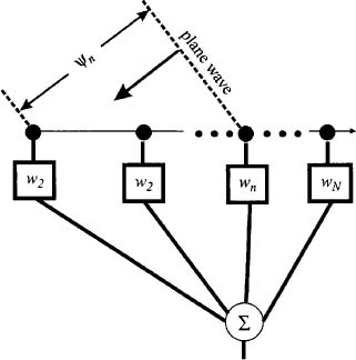
Figure 2.3. Diagram of a linear array.

Figure 2.4. Arbitrary distribution of elements in the x−y plane.

where

(x_n, y_n) = location of element n                             
u = sin θ cos                                                    
v = sin θ sin                                                     
w = cos θ                                                          
u² + v² + w² = sin² θ(sin² + cos² ) + cos² θ ≤ 1

The array factor is a function of amplitude weights, phase weights, element placement, and frequency. This chapter examines the effects on the array factor due to varying these variables. The next chapter provides recipes for finding the values of these variables that produce a desired array factor.

2.1.1. Phase Steering

The maximum value of the array factor is at the peak of the main beam which occurs when ψ_n = 0 for all n.

Figure 2.5. Beam of an 8-element array steered to 45°.

This maximum can be moved without moving the antenna by adding a con stant phase shift, δ_n, to ψ_n. For a linear array along the x axis, the phase at element n is

If δ_n is selected such that ψ_n = 0° in the desired steering direction, u_s, then the peak of the main beam will appear at u = u_s.

Phase shifters placed at each element implement the steering phase.

Example. Consider an 8-element uniform array along the x axis with an element spacing of 0.5λ. Steering its beam to an angle of = 45° (Figure 2.5) requires a phase at element n of δ_n= −.707π (n − 1) radians.

A phase shift only delays a signal by up to one period or 2π radians. If the signal received at the first element is within the same period as the signal received at the last element, then

Thus, one pulse width can illuminate the entire aperture at once when it is incident from the maximum steering angle. Technically, to reproduce the signal with 100% accuracy, time delay units (δ_n > 2π) would be required whenever (2.8) is violated. A phase shifter only delays a signal up to one period, T, while a time delay unit can delay the signal many periods. In practice, the rule of thumb is to use time delay units whenever the first element of the array receives the beginning of the pulse and the last element of the array receives the end of the pulse [1].

where τ_3dB is the pulse width and c is the speed of light.

Example. A 60-element uniform linear array with d = 1.5 cm at 10 GHz receives a pulse having a bandwidth of 100 MHz. What is the maximum scan angle without time delay units?

which means that the main beam is limited to scanning ±19.9° off broadside.

The phase shift required at element n in a planar array to steer a beam to (_s, θ_s) is

where . The phase in (2.10) reduces to that of a linear array if the beam is steered in one of the principal planes (either = 0° or = 90°).

Figure 2.6 shows the effects on the array factor in three dimensions as it is steered from 90° to 0°, assuming that the 8-element linear array lies along the x axis and has a constant λ/2 element spacing. The array factor starts with a doughnut shape at broadside and ends with a dumbbell shape at end-fire.

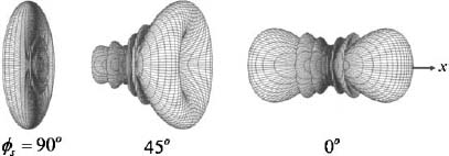
Figure 2.6. Beam of an 8-element linear array steered from 90° to 0° in three dimensions.

2.1.2. End-Fire Array

An end-fire array is a linear array having the peak of its main beam pointing in the same direction as the axis of the array. The simplest end-fire array is a uniform array with its peak steered to u = 1 (see 0 degrees in Figure 2.6), which means that ψ = 0° or

A polar plot of the array factor for an end-fire array with N = 5 and d = λ/2 is shown as the solid line in Figure 2.7. This array factor has a very wide beamwidth and two main beams. Shrinking the element spacing to 0.2λ produces the dashed line in Figure 2.8. The closer spacing eliminates the main beam at 180°.

A narrower main beam, hence better resolution and a higher directivity, is possible by altering the spacing and phase in an optimal fashion. The Hansen–Woodyard end-fire array [2] achieves greater directivity by forcing the maximum of the main beam to be in invisible space or u > 1. An optimum directivity occurs when an extra π phase shift occurs across the extent of the array. This optimum phase shift is given by

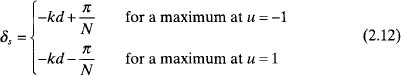
Figure 2.7. Polar plot of the array factors of an end-fire array for d = 0.5λ and d = 0.2λ.

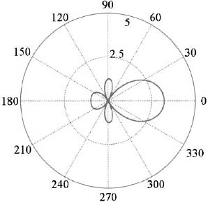
Figure 2.8. Polar plot of the array factors of a Hansen–Woodyard end-fire array for optimum spacing (d = 0.2λ).

when the array element spacing is

which for large arrays becomes

Figure 2.8 is the Hansen–Woodyard end-fire array factor with d = 0.2λ for a 5-element array.

2.1.3. Main Beam Steering with Frequency

If the main beam of the array is pointing at an angle of u_s due to phase steering the main beam, then the peak of the main beam will move with a change in frequency. As a result, the main beam can be steered without moving the array.

Example. At 10 GHz, the elements of a linear array are spaced 0.5λ and the array operates from 8.2 to 12.4 GHz.

The phase delay between elements is then given by δ_s = 0.79 radians. This phase shift steers the beam to an angle of

      from broadside

At 8.2 GHz (λ = 3.66 cm), the beam points at u_s = 0.305 = 17.8°.

At 12.4GHz (λ = 2.42cm), the beam points at u_s = 0.202 = 11.7°

2.1.4. Focusing

Focusing an array concentrates the field radiated/received by the array at/from a specific point in the near field rather than the far field. Antenna focusing has been applied to antenna measurements [3] and medical treatments [4]. The focusing occurs over a small area rather than at a single point due to the finite aperture size. Ricardi [5] and Hansen [6] show that the minimum spot size of a uniform array antenna is about 0.35λ in diameter. Since the focal point is in the near field, the array factor must take into account the exact distance from each element to the focal point at (x_f, y_f). The relative array factor in the near field is given by

where . In order to focus the array, the array factor should coherently sum to a maximum at the focal point. In other words, the phase of the field from each element is made identical at the focal point by setting the weights to

Focusing an array results in the highest possible field level at the focal point without any amplitude weighting.

Example. Find the phase weights of an 8-element array centered at x = 0 with d = 0.5λ that has a beam focused at x = −0.5λ and y = 2λ. Compare results with an unfocused array.

The phase weights (in radians) needed to focus the array are

[−2.25   −0.85   −0.0978   −0.0978   −0.855   −2.25 2.15    −0.0653]

Figure 2.9 shows the near-field array factor for the array focused at (x_f,y_f) = (−0.5λ,2λ). The power is much higher (10.8 dB) than if the far-field beam is steered in the direction of the focal point (1.9 dB) as shown in Figure 2.10.

Figure 2.9. Near-field array factor when array is focused in the near field at (x_f, y_f) = (−0.5λ, 2λ).

Figure 2.10. Near-field array factor is focused in the far field at (x_f, y_f) = (−50λ, 200λ).

2.2. UNIFORM ARRAYS

Uniform arrays have periodic element spacing, and the weights at each element are the same, except for beam-steering phase shifts.

2.2.1. Uniform Sum Patterns

A uniform linear sum array has w_n = 1 and equally spaced elements with the peak of the main beam pointing at broadside. Assuming the phase center is at the first element of the array, then the array factor is given by

where

The distance a plane wave needs to travel between adjacent elements along the x axis is shown in Figure 2.11. Multiplying the distance by k yields the phase, ψ. A similar derivation is possible when the array lies along the y or z axes.

The phase reference does not have to be the first element in the array. Moving the phase reference results in multiplying the array factor by a

Figure 2.11. Phase difference between adjacent elements of a uniform linear array along the x axis.

constant phase but will not change the magnitude of the array factor. Another convenient place for the phase reference is the physical center of the array. When the origin of the coordinate system moves to the center of the array, the array factor becomes

Equations (2.17) and (2.18) differ only by the phase factor

which is the phase difference between element 1 and the center of the array.

Multiplying both sides of (2.17) by e^jψ and subtracting the resulting product from (2.17) results in a simpler expression for the array factor

Solving (2.20) for AF produces

The maximum of (2.21) occurs when ψ = 0°.

Often, only the relative array factor is important, and dividing (2.21) by N normalizes the array factor. If the phase center is at the physical center of the array, then the phase term in (2.21) disappears. Thus, the array factor normalized to the peak of a uniform array factor (N) when the phase center is at the physical center of the array is

Note that the denominator in (2.21) is independent of array size and forms an envelope for the array factor amplitude, because it has a lower frequency than the numerator. On the other hand, the frequency of the sine wave in the numerator is proportional to the number of elements in the array. A comparison of the array factors and numerators for N = 10 and N = 20 is shown in Figure 2.12. The dotted line in the figure is the envelope or denominator and is the same for both arrays.

Figure 2.12. Uniform array factors for N = 10 and N = 20 along with the numerators and denominator of the expression for the uniform array.

The zeros of (2.23) or nulls in the array factor occur when AF_N(ψ_null) = 0, and the denominator is not equal to zero or

Sidelobes are local maxima that occur between two nulls. Their approximate location occurs when the numerator of (2.23) is a maximum or

For a large array, the numerator of (2.23) quickly varies while the denominator slowly varies. The first sidelobe occurs at a small value of ψ; and the small argument approximation for sin, or x ≃ x for small values of x, is used in the denominator. Consequently, the sidelobe envelope close to the mainbeam is given by the denominator of (2.23). Substituting the location of the first sidelobe into (2.23) provides an estimate of the sidelobe level of the first sidelobe of a uniform linear array.

Figure 2.13. Array factors for N = 4-, 6-, and 8-element arrays having elements spaced d = λ/2 along the x axis.

Smaller uniform linear arrays have sidelobe levels close to 13 dB below the peak of the main beam.

Example. Plot the unnormalized array factors for N = 4-, 6-, and 8-element arrays having elements spaced d = λ/2 along the x axis.

Figure 2.13 shows the three array factors. Increasing the number of elements increases the main beam peak and the number of sidelobes and decreases the width of the main beam.

As mentioned in Chapter 1, the antenna beamwidth determines the resolution and gain of the array. A useful approximation for the null-to-null beam-width for a uniform array comes from (2.24) with m = 1

In most electromagnetics systems, the 3-dB beamwidth is more useful than the null-to-null beamwidth. It is found by taking the difference between the two angles found by solving the following transcendental equation:

When N is large, then the argument in the denominator is small, so the array factor can be approximated by a sine function, and the the 3-dB beamwidth is found by

The 3-dB point on a sinc function is given by

For half-wavelength spacing the 3-dB beamwidth is approximately twice the angle found in (2.30).

Example. Find all the maxima and nulls for a 6-element array having elements spaced d = λ/2 along the x axis. What is the null-to-null and 3-dB beamwidths?

The 3-dB beamwidth is found by finding the angles for which

This value is quite close to that obtained using (2.31), (θ_3dB ≃ 16.9°.

A planar array can be constructed by stacking linear arrays. Start with an N_x1 element linear array along the x axis with element spacing d_x and weights W_1n. Another linear array having N_x2 elements is placed d_y above the first array and displaced Δ₂ in the x direction. Linear arrays are added d_y above the last one until the planar array is complete (see Figure 2.14). The array factor for this array is given by

Figure 2.14. Planar array can be built from a set of equally spaced linear arrays.

where N_y is the number of linear arrays, N_xm is the number of elements in linear array m, and Δ_m represents x displacement of array m.

Two common element layouts are rectangular spacing

and triangular or hexagonal spacing [7]

These spacings for a rectangular array are shown with two microstrip arrays in Figure 2.15. The array on the left has 16 elements in a rectangular lattice within a square boundary and operates at X band. The array on the right has 19 elements in a triangular lattice within a hexagonal boundary and operates at L band. Although the equilateral triangle spacing is most common, isosceles and general triangular spacing is also possible [8].

If all the weights are equal to one, then the array factor for rectangular spacing is

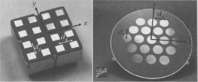
Figure 2.15. Common element lattices for a planar array. (Courtesy of Ball Aerospace & Technologies Corp.)

where

ψ_x = kd_x(u−u_s)
ψ_y = kd_y(v−v_s)

and for triangular spacing is

The triangular spacing array factor consists of two uniform arrays with spacings of 2d_x and 2d_y. The first array has its bottom left element at the origin, and the second array has its bottom left element at (d_x, d_y).

Usually, the beamwidth of a planar array is defined for two orthogonal planes. For example, the beamwidth is usually defined in θ for = 0° and = 90°. As with a linear array, nulls in the array factor of a planar array are found by setting the array factor equal to zero. Unlike linear arrays, the nulls are not single points.

2.2.2. Uniform Difference Patterns

A difference pattern has a null at broadside instead of a peak. This null can precisely locate the direction of a signal, because the null has a very narrow angular width compared to the width of the main beam of a corresponding sum pattern. When the array output is zero, the signal is in the null. Slight movement of the null dramatically increases the gain of the array factor and the reception of a signal. A 20-element uniform sum array can be converted into a 20-element difference array by giving half the elements a 180° phase shift, or half the elements are one and half are minus one. The array factor for this uniform difference array is shown in Figure 2.16.

The array factor for a uniform difference array is written as

Figure 2.16. Twenty-element uniform difference array factor normalized to N.

Multipling both sides of (2.37) by e^jψ and subtracting the resulting product from (2.37) results in a simpler expression for the array factor

Solving (2.38) for AF produces

Moving the phase center to the middle of the array reduces (2.39) to

Nulls occur when

Sidelobes in the array factor approximately occur when the numerator is a maximum.

Figure 2.17. Plot of the magnitude of the ratio of the sum and difference patterns for a 2-element uniform array from θ = −30° to 30°.

This equation does not yield a good approximation to the height of the difference main lobes; hence n starts at one instead of zero.

Example. Plot the magnitude of the ratio of the sum and difference patterns (DF) for a 2-element uniform array from θ = −30° to 30°.

Figure 2.17 has a plot of the ratio, DF, (solid line) and a linear fit of DF (dotted line). This plot shows that the angle of incidence can be found from the ratio of the difference pattern to the sum pattern.

2.3. FOURIER ANALYSIS OF LINEAR ARRAYS

Antenna arrays sample the signals incident on them through elements at discrete locations. In order to avoid aliasing, the array must sample the incident signal at the Nyquist rate. The Nyquist rate stipulates that two samples are taken during the period of the highest frequency. Since an electromagnetic signal has time (T) and spatial (λ) periods, the samples are taken at

Figure 2.18. Array sampling of plane wave from three directions.

Of course, these are related by

where c is the speed of light. Consequently, the elements of an array must be separated at most by half a wavelength to avoid under sampling an incident plane wave for any angle of incidence. A plane wave impinges on all the elements of an array simultaneously at normal incidence (Figure 2.18a). At this angle (u = 0) the element spacing is irrelevant. Figure 2.18b demonstrates the need for λ/2 sampling for an incoming wave from the u = 1 direction. Undersampling is not a problem at normal incidence but can be at angles off-normal. The angle at which aliasing begins (Figure 2.18c) is given by u_A. This wave is sampled at the Nyquist rate if

Thus,

Aliasing manifests itself as pattern replication. As the spacing gets wider, grating lobes or clones of the main beam appear in the pattern. These extra main beams appear at regular intervals given by

Figure 2.19. Array factors of 8-element arrays for three different spacings.

When the array with grating lobes receives a signal, the direction of the signal cannot be determined, because the angle of arrival is ambiguous: Did the signal enter the main beam or the grating lobe? The broadside array factors of an 8-element array with element spacings of d = λ/2, d = λ, and d = 2λ are shown in Figure 2.19. Increasing the frequency causes d/λ to increase as well. An array designed for optimum sampling at the center frequency undersamples a plane wave at frequencies above the center frequency and oversamples at frequencies below the center frequency.

Example. An array operating at a center frequency of f₀ = 10 GHz (λ₀ = 3 cm) has a 5% bandwidth. What is the maximum element spacing (in centimeters) that adequately samples signals up to ±30° from broadside?

The highest frequency will limit the element spacing, so f = 10.25 GHz and

An equally spaced linear array is the superposition of many 2-element arrays. If the amplitude weights are symmetric about the center of the array, then symmetric pairs of exponent terms in the array factor can be combined into a cosine term. An even element array has N = 2M elements and an odd-element array has N = 2M+1 elements. The symmetric elements in an odd array with the phase center at the physical center of the array combine as follows:

Figure 2.20. A 6-element array is composed of three Fourier components added together. The 6-element array is shown at the top. Pairs of elements point to their corresponding array factors.

The array pattern, then, is the superposition of all the 2-element array patterns that make up the array. Figure 2.20 has plots of the three Fourier components of a 6-element array superimposed on the array factor for a 6-element uniform array. At u = 0, the three components have peaks that add in phase to form the main beam. If an array has an odd number of elements, then there is a single element at the center (zero spatial frequency) with an amplitude weight a₀. The array factors for the even- and odd-element arrays can be written as

These equations have the familiar form of a Fourier series, especially when written as

A difference pattern with low sidelobes requires a different set of weights than a corresponding sum pattern. The amplitude taper for sidelobes in a sum pattern will not result in the same low sidelobes in a difference pattern and vice versa. Difference arrays have an even number of elements, because the center element of an array with an odd number of elements serves as a constant in the Fourier series. This constant would not be canceled by the other elements, so the difference null would not be as deep. The array factor for a symmetric linear difference array is given by

where b_n is the difference amplitude weight for element n.

The fast Fourier transform (FFT) is an efficient way to calculate the array factor. Usually, the antenna weights are placed in an array then padded with zeros (zeros added onto the end of the array weights). For instance, if there are N elements in the array and P zeros used for padding, then the vector looks like

The number of zeros in the pad determines how smooth the array factor will look. Basically, the interpolation in u space is in increments of Δu = 2/(N + P) from u = −1 to u = (N + P)Δu−1. Note that u = 1 is not included. This fact is important in relating the FFT results to points in space.

Example. Find the array factor of an N = 8 element uniform linear array using a FFT.

The MATLAB command is given by

An FFT algorithm usually returns the dc component in the first cell of the vector. A command like fftshift rearranges the vector to put the dc component in the center. As the number of zeros in the pad increases, the array factor becomes smoother. Figure 2.21 shows the FFT array factor for P = 0,8, 24, and 56.

2.4. FOURIER ANALYSIS OF PLANAR ARRAYS

The elements of a planar array are usually laid out in a periodic lattice in the x−y plane. For example, when elements are in a rectangular lattice, (2.32) is written as a two-dimensional discrete Fourier series

Figure 2.21. FFT of an 8-element uniform linear array with P = 0,8,24, and 56.

Figure 2.22. Grating lobe plot for a rectangular array.

Figure 2.22 is a plot of the maxima of (2.53) as a function of u and v and is known as a grating lobe plot. The three dashed lines correspond to the angular space 0 ≤ θ ≤ 90° and 0 ≤ ≤ 306° (real space) when d_x = d_y = λ/2, λ, and 1.5λ. If the element spacing is not the same or the number of elements are different in the x and y directions, then the circles in the u−v plane are ellipses. For the rectangular element spacing, grating lobes appear at regular intervals given by

All grating lobes in (2.54) that satisfy

appear in the array factor in real space. As can be seen from (2.55), steering the main beam moves the center of the circle in the u−v plane to the point (u_s, v_s). A planar array (with no steering) in the x−y plane with uniform spacing sees the grating lobes enter real space at θ = 90° and φ = 0°, 90°, 180°, 270° when d = 1.0λ in the x and y directions. When d = 1.41λ, then additional grating lobes enter real space at the 45°, 135°, 225°, and 315° azimuth angles as shown in Figure 2.22.

Triangular spacing modifies the sampling strategy and produces grating lobes at the locations (u_m, v_n) defined by

The spacing d_x is the length of the bottom side of the triangle, while d_y is the height of the triangle. Only grating lobes that satisfy (2.55) appear in the array factor. The grating lobe plot for equilateral triangular spacing is shown in Figure 2.23. The first set of six grating lobes appear in real space when which is larger than the minimum spacing for grating lobes for rectangular element spacing. Grating lobes enter real space at θ = 90° when φ = 30°, 90°, 150°, 210°, 270°, 330°. The element spacing in those directions is 2d_y. Since for an equilateral triangle, then in those six directions

and grating lobes appear. Thus, we would expect grating lobe peaks to enter real space when the element spacing between elements in any row (x direction) to be . Now grating lobes at φ = 0°, 60°, 120°, 180°, 240°, and 300° due to element spacings in the x direction should occur when d = 2.0λ as verified by Figure 2.23.

Figure 2.23. Grating lobe plot for triangular spacing.

Triangular spacing not only delays the appearance of grating lobes but allows larger elements in the array. The maximum area that an element can occupy in rectangular spacing is d_xd_y while for triangular spacing it is . As a result, an array with triangular spacing has 86.6% fewer elements than the same array with a square lattice. At least from a throretical point of view, triangular spacing is superior to rectangular spacing. Practical considerations, such as the feed network, may dictate the need for rectangular spacing.

Grating lobes appear in directions where the periodic sampling is one wavelength or more. By controlling the sampling in certain directions through varying Δ_m, d_x, and d_y in (2.32), the grating lobes can be moved to a direction that can accommodate limited scanning without bringing the grating lobes into real space [9]. Another approach is to randomize the Δ_m, so there is no periodic spacing in any direction.

The element lattice that samples the received signal occurs inside a defined perimeter or shape. The three most common planar array shapes are rectangular (including square), elliptical (including circular), and hexagonal. Figure 2.24 has examples of hexagonal, circular, elliptical, and rectangular arrays. Other shapes, including fractal, have also been used. Oftentimes, the shape must conform to the surface area available. For instance, the AN/APG-77 radar antenna shown in Figure 2.25 fits inside the nose cone of a USAF F-22A. It has 1500 elements arranged in an irregular shape. Grating lobes are a function of the periodic spacing of the elements and not the array shape. Directivity of an array factor is a function of array area but not shape. The shape does play an important role in determining beamwidth and sidelobe level of the array factor, however.

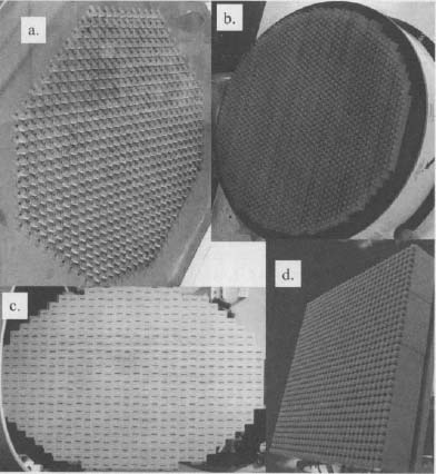
Figure 2.24. Some planar array shapes: a. hexagonal b. circular c. elliptical d. rectangular. (Courtesy of Northrop Grumman and available at the National Electronics Museum.)

Figure 2.25. AN/APG-77 radar array. (Courtesy of Northrop Grumman and available at the National Electronics Museum.)

The element locations inside any shaped boundary can be found by first selecting an element lattice (rectangular or triangular) that is larger than the desired array. Next, overlay the array shape on the element lattice. Elements in the lattice that are outside of the shape are discarded. Certain element configurations can be generated without this process, such as rectangular arrays and fractal arrays.

Example. Compare the uniform array factors for a square, circle, and hexagon-shaped planar array with rectangular element spacings of d_x = d_y = 0.5λ.

The element layouts and corresponding uniform array factors appear in Figure 2.26 to Figure 2.31. The square array has the highest sidelobes. They only occur in two directions of , however. Outside of those two cuts, the sidelobes are extremely low. The circular array has nearly constant sidelobes as a function of , especially close to the main beam. Its peak sidelobes are lower than those of the rectangular array. The hexagonal array has its highest sidelobes along four cuts in the direction. Directivity is nearly the same for all the shapes, since they have about the same number of elements. Table 2.1 lists the directivity and maximum sidelobe level for square, circular, and hexagonal arrays in Figures 2.26−2.31.

When the elements lie on a rectangular grid, then the array factor takes the form of a two-dimensional DFT. The two-dimensional FFT can be used to

Figure 2.26. Square array with rectangular spacing.

Figure 2.27. Array factor for the square array.

Figure 2.28. Circular array with rectangular spacing.

calculate an array factor [10]. Zero padding is necessary in both rows and columns of the weight matrix in order to get sufficient sampling. In this case, both u and v are a function of θ and , so there is not a nice relationship between the Fourier transform variable and an angle as in the case of a linear array.

Figure 2.29. Array factor for the circular array.

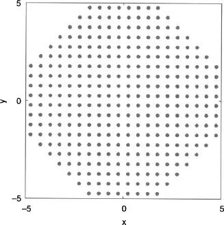
Figure 2.30. Hexagon array with rectangular spacing.

Example. Calculate the array factor of the triangular array in Figure 2.32. The array has 36 elements on a rectangular grid with d_x = 0.5λ and d_y = 1.0λ.

A DFT multiplies a row vector of N element weights with N × N_ang phase matrix. This results in about N × N_ang operations. To invoke an FFT, the weight matrix is filled with zeros in order to make the weight matrix rectangular. Next, the weight matrix is padded with zeros in order to sufficiently interpolate the array factor so that it looks smooth when graphed. Figure 2.33 is the array factor calculated using the FFT. The array factor points outside the circle are ignored, because they are associated with physically impossible angles. They account for (1-π)/4×100% or 21.5% of all the points calculated.

Figure 2.31. Array factor for the hexagon array.

TABLE 2.1. Characteristics Dure to Planar Array Shapes when Elements Are in a Square Grid

2.5. ARRAY BANDWIDTH

The array bandwidth is determined by a number of factors:

1. Bandwidth of the elements in the array
2. Element spacing
3. Maximum steering angle
4. Array size

Figure 2.32. Weight matrix for triangular array for N = 36, d_x = 0.5λ, and d_y = 1.0λ.

Figure 2.33. Array factor calculated using an FFT. The points outside the circle should be ignored.

The bandwidth of the elements will be discussed in Chapter 4. The other three factors can be examined using isotropic point sources. Increasing the frequency increases the sampling in terms of wavelength between elements. As a result, the grating lobes appear sooner for higher frequencies than for lower frequencies as indicated by (2.54) and (2.56). Element spacing and grating lobe formation sets an upper frequency limit to the bandwidth.

As presented earlier, when a beam is scanned, a change in frequency causes a change in main beam pointing direction. The main beam shift as a function of frequency is most pronounced at the highest scan angle. At frequency f, the main beam squints (moves) from u_s = sin θ_s at f₀ = center frequency to angle u_squint = sin θ_squint according to

Note that u_squint gets smaller for frequencies higher than f₀ and smaller for frequencies less than f₀. If f_hi and f_1o define the upper and lower limits of the bandwidth, then for a constant phase shift between element (steering phase)

The angular difference between the upper and lower frequencies is given by

Figure 2.34 is a plot of the steering angle as a function of frequency for θ_s = 10°, 20°, 30°, 40°, 50°, 50° at f_lo. The change in beam pointing direction over the same frequency range increases as θ_s increases.

Increasing the size of an array decreases its bandwidth. If the bandwidth is bound by a 3-dB reduction in the main beam, then the bandwidth is calculated by

Figure 2.35 is a plot of the array bandwidth as a function of the center frequency for array sizes with N = 20, 40, 60, and 100 for a uniform array with d = 0.5λ. A good approximation for the bandwidth is given by [1]

Figure 2.34. Plot of steering angle as a function of frequency.

Figure 2.35. Array bandwidth as a function of steering angle and array size.

2.6. DIRECTIVITY

To find the directivity of an array, substitute the array factor into the equation for directivity in Chapter 1.

A linear array with arbitrary element spacing along the z axis is symmetric with respect to , so the integral with respect to in the denominator reduces to 2π, and the directivity becomes

The integral in (2.64) is easy to numerically compute. If the elements have a constant spacing, d, then an analytical form exists [20]:

where sine (x) = sin (x)/x. If the elements are spaced 0.5λ apart, then the directivity formula simplifies to

Uniform arrays with constant spacing have a directivity of

When d = 0.5λ, the directivity becomes

Figure 2.36. Directivity of a uniform linear array as a function of element spacing.

Graphs of the directivity as a function of element spacing for several values of N are shown in Figure 2.36. The directivity increases until a grating lobe appears (d is a multiple of λ), and then it sharply decreases. This decrease is due to an increase in the denominator while the maximum value of AF in the numerator remains the same. The decrease in directivity due to the grating lobe becomes more dramatic as the number of elements increases, because the main beam and grating lobes have narrower beamwidths: A small change in θ produces a large change in AF.

Weighting the elements in the array reduces the directivity and efficiency of the array. A weighted aperture collects less total electromagnetic waves than a uniformly weighted aperture, so it is less efficient. Taper efficiency (also called illumination or aperture efficiency) is the ratio of the directivity of the tapered array to that of a uniform linear array or

When d = 0.5λ, this equation simplifies to

Taper efficiency is an important figure of merit when evaluating low sidelobe tapers.

The directivity for a planar array is found by substituting (2.4) into (2.63) to get

It is unusual to have a planar array radiate out the front and back, so the limit of integration for θ only goes from 0° to 90°, because the pattern is zero from θ equals 90° to 180°. Note that this assumption was not made for the linear array. Some terms in the denominator can be pulled outside the integrals to get

The integrals in the denominator can be evaluated analytically for certain element spacings, such as rectangular. Directivity formulas tend to be quite complicated and severely restricted to the element layout [20]. Performing the numerical integration in (2.72) is relatively easy and has the advantage of being geometry-independent.

Many approximate formulas exist for quickly estimating the directivity of an array. First, the directivity can be calculated from the projected area of the array (A_p) as long as the element spacing is not much larger than 0.5/λ:

If the array has an irregular shape, then assume that each element occupies an area equal to d_xd_y for rectangular spacing. Thus, an N element array has an approximate directivity given by

Separable apertures are rectangular planar arrays whose array factors can be written as the product of two linear arrays and have an approximate directivity of

where D_x is the directivity of the linear array in the x direction and D_y is the directivity of the linear array in the y direction. The directivity can also be estimated if the 3-dB beamwidths are known in orthogonal directions.

where is the 3-dB beamwidth in degrees at = 0°, is the 3-dB beamwidth in degrees at = 90°, is the 3-dB beamwidth in radians at = 0, and is the 3-dB beamwidth in radians at = π/2. These formulas result from approximating the 3-dB beamwidth by λ/(Nd). When the array scans its beam, then the directivity decreases due to the decrease in the projected area of the array.

Example. Find the directivity of a rectangular planar array with N_x = 6, N_y = 10, d_x = 0.5, and d_y = 0.7 using (2.72) and (2.73) for both a uniform aperture and an aperture that is uniform in the y direction and has the amplitude weights [0.541 0.777 1 1 0.777 0.541] in the x direction.

The taper efficiency for this array is 0.944.

Since grating lobes can enter space from more than one direction, the directivity of a planar array has more abrupt changes as the element spacing increases than a linear array. Figure 2.37 has plots of directivity versus element spacing in λ for a square array of 10 by 10 elements with square and hexagonal element lattices. These curves relate to the grating lobe plots in Figures 2.22 and 2.23. The square spacing has its first minimum at d = 1.0λ and the second at d = 1.4λ. The hexagonal spacing has its first minimum at d = 1.15λ and the second at d = 2.0λ.

2.7. AMPLITUDE TAPERS

The element weights control the directivity and sidelobe level of the array factor. Low-sidelobe amplitude tapers have high amplitude weights in the center of the array. The weights generally decrease from the center to the edges. Some examples are shown in Table 2.2. The results in Table 2.2 were obtained through numerical simulations (also see reference 11. The sidelobe levels and taper efficiencies assume that Nd is large. As the taper efficiency decreases, the 3-dB beamwidth increases and sidelobe levels decrease.

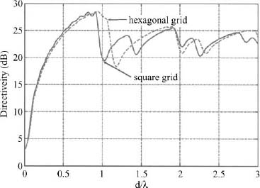
Figure 2.37. Directivity of planar arrays as a function of element spacing.

TABLE 2.2. Properties of Some Simple Low-Sidelobe Amplitude Tapers for a Linear Array with Large Nd [11]

Example. Plot the array factors for a 20-element d = 0.5λ array with triangular, cosine, and cosine-squared amplitude tapers.

Figure 2.38 shows the three low sidelobe array factors superimposed. The beamwidths and first sidelobe levels are shown in Table 2.3.

Figure 2.38. Array factors for a 20-element d = 0.5λ array with triangular, cosine; and cosine-squared amplitude tapers.

TABLE 2.3. Array Factor Characteristics for Three Low-Sidelobe Amplitude Tapers

2.8. z TRANSFORM OF THE ARRAY FACTOR

The z transform converts the linear array factor into a polynomial using the substitution [12]

Substitute z into (2.17) to get

It is convenient to write the array factor in (2.79) as

Factoring the above polynomial yields

Each root (z = z_n) corresponds to a null in the array pattern. The roots have a magnitude of one and phase of ψ_n. A 4-element uniform array with d = 0.5λ has the following polynomial form:

Its roots are graphed on the unit circle in Figure 2.39, and the array factor is shown in Figure 2.40.

The magnitude of the array factor between zeros relates to the angular separation of the zeros. Closely spaced zeros have small lobes between them, while widely spaced zeros have large lobes between them. The uniform array example has zeros 1 and 2 and zeros 2 and 3 closely spaced, while zeros 1 and 3 are widely spaced. The array factor between the closely spaced zeros are sidelobes, and the array factor between the widely spaced zeros is the main beam. Thus, the sidelobe levels of the uniform array may be lowered by moving the zeros on the unit circle as shown in Figure 2.41. For instance, moving the zeros of the 4-element uniform array closer to the negative real axis lowers the pattern’s sidelobe levels and widens the main beam. Null locations at ψ = ±120° instead of ψ = ±90° result in

Figure 2.39. Unit circle representation of a four element uniform array.

Figure 2.40. Array factor of a four element uniform array with d = 0.5λ.

Figure 2.41. The zeros are moved closer together on the unit circle.

The amplitude weights for the array elements are 1,2,2, and 1. These weights produce the normalized low-sidelobe array factor shown in Figure 2.42. Note that the sidelobes are lower and the main beam is wider than those of the uniform array.

The examples so far only considered zeros lying on the unit circle. What happens to the array factor when the zeros move off the unit circle. The four element array has roots at z = −1 and ±j as indicated by the zeros labeled with a 1 in Figure 2.43. Changing the roots to z = −1.2 and ±1.2j moves them a radial distance of 0.2 outside of the unit circle as shown by the zeros labeled with a 2 in Figure 2.43. The corresponding array weights are real since the roots are complex conjugate pairs and not symmetric: w = [0.5787 0.6944 0.8333 1.0]. Moving the roots off the unit circle by an additional 0.2 results in roots at z = −1.4 and ±1.4j which are labeled by a 3. The corresponding array weights are real since the roots are complex conjugate pairs and not symmetric: w = [0.3644 0.5102 0.7143 1.0]. The effects of moving the zeros is apparent on the array factor shown in Figure 2.44 and include

Figure 2.42. Moving the zeros closer together on the unit circle lowers the sidelobes and expands the main beam.

Figure 2.43. Zeros moved off the unit circle for a 4-element array.

Figure 2.44. Array factors corresponding to zeros moved off the unit circle.

• Decreased directivity and efficiency
• Increased relative sidelobe levels
• Filled-in nulls

Moving zeros inside the unit circle produces similar effects to the array factor. For instance, moving the roots to z = −0.8 and ±0.8j results in the exact same amplitude weights as when z = −1.2 and ±1.2j, and the array factor looks like the plot labeled 2 in Figure 2.44.

2.9. CIRCULAR ARRAYS

A circular or ring array with elements lying on a circle of radius r_c in the x−y plane has an array factor given by

where _n is the angular location of element n. The beam is steered by applying a phase at element n given by

Normally, the elements are equally spaced around the circle, so they are separated by an angle

As a result, the radius of the circle and the arc distance between adjacent elements is given by

If r_c is known, then d can be found, or if d is known then r_c can be found. If the array weights are uniform, then the array factor can be written as [13]

where and J_n is a Bessel function of order n. The principal component is the n = 0 term, and all other terms are referred to as residuals. For large arrays, the principal component is the dominant term, and the residuals can be ignored. Thus, for a large radius, the array factor is approximately

If several circular arrays with different radii share a common center, then the resulting planar array is known as a concentric ring array [14,15]. Figure 2.45 is a diagram of a concentric ring array with ring n having N_n elements and a radius of r_n. The physical distance between elements on ring n is constant and given by d_n. Ring arrays are either designed to have a main beam at θ = 90° and scan only in azimuth or have a main beam at θ = 0° and scan in azimuth and elevation.

The array factor for the concentric ring array with a single element at the center (Figure 2.45) is given by

where N_n is the number of elements in ring n, N_r is the number of rings, w_n represents elements weights for ring n, r_n is the radius of ring n, (x_n, y_n) is the location of element n, x_n = r_ncos_m, y_n = r_nsin _m, and _m = 2π(m−1)/N_n. In this formula, all the elements in the same ring have the same weight.

Figure 2.45. Diagram of a concentric ring array.

The array factor for a circular array is often written in terms of Bessel functions as shown in (2.88). If each ring is represented by (2.88), then (2.90) can be rewritten as [13]

Assuming that all the radii are large, then the array factor is independent of and only the principal component terms for each ring remain.

Figure 2.46 is a diagram of a 279-element concentric ring array. There are nine rings with r_n = nλ/2 and d_n = λ/2. The number of equally spaced elements in ring n is given by

Since the number of elements must be an integer, the value in (2.93) must be rounded up or down. To keep d ≥ λ/2, the digits to the right of the decimal point are dropped. Table 2.4 lists the ring spacing and number of elements in each ring for a uniform concentric ring array with nine rings as shown in Figure 2.46.

Figure 2.46. Concentric ring array with nine rings spaced λ/2 apart and having d_n ≃ λ/2.

TABLE 2.4. Ring Radius and Number of Elements per Ring for a 9-Ring Uniform Concentric Ring Array

A uniform array has equal element spacing and weighting. For a uniform concentric ring array, the ring spacing, r_n, is a constant times the ring number and the spacing between elements within a ring, d_n, is approximately constant for all rings. A nine-ring concentric ring array has the array factor shown in Figure 2.47. The Bessel function behavior in (2.92) is quite evident in the array factor. It has a directivity of 29.4 dB, a peak sidelobe level of −17.4 dB, and is symmetric in . As long as the array factor is predominantly a function of θ, the maximum can be found from a slice of the array factor for a single value of .

2.10. DIRECTION FINDING ARRAYS

Direction finding with linear arrays is limited to either the θ or directions. In order to direction find in both azimuth and elevation directions, a planar array is needed. Circular arrays are also commonly used for direction finding.

Figure 2.47. Array factor due to the array with nine concentric uniform rings.

Figure 2.48. Diagram of a 4-element Adcock antenna.

2.10.1. Adcock Array

The original Adcock array has four uniformly weighted elements situated at the four corners of a square with sides less than λ/2 (Figure 2.48) [16]. It was developed to find the direction of arrival of a signal in both azimuth and elevation. The north (N) and south (S) antennas on the y axis are out of phase, and the east (E) and west (W) antennas along the x axis are out of phase as well. The N−S array has an array factor given by

Likewise, the array factor for the E−W array is given by

Sir Watson-Watt developed the principle for finding the elevation and azimuth of a source incident on an Adcock array [17]. An estimate of the tangent of the azimuth angle is the ratio of the output from the E−W array to the output of the N−S array.

An estimate of the elevation angle is given by

More accurate estimates of the arrival angles are possible by adding element pairs to the 4-element Adcock antenna on opposite sides of a circle with a center at the origin of the x−y axes.

2.10.2. Orthogonal Linear Arrays

A planar array is needed to locate sources in both azimuth and elevation. The Adcock array is the simplest version. Adding more elements to an array increases the cost of the components and computational complexity of the signal processing algorithms. As a result, direction of arrival (DOA) arrays have just enough elements to locate a desired number of sources. Orthogonal linear arrays are often used in place of fully populated arrays for direction finding [18].

The array factor for the linear array along the y axis can be written as a polynomial.

where z_y = e^jψy. A similar polynomial for AF_x is written in terms of z_x = e^jψx. The polynomials for orthogonal arrays along the x and y axes can be factored to find the zeros:

If several signals are incident upon the array, then the weights are adjusted until the array output is minimized. Factoring the array factor polynomial yields the polynomial zeros, hence the location of the nulls and the incident signals. The azimuth angle of a null is found by [19]

or

The elevation angle is found from

Solving for θ₁ yields

Once the zeros of the array factor polynomials are known, then the source locations in (θ₁, ₁) can be found.

2.11. SUBARRAYS

Large phased array antennas are often divided into many smaller subarrays. The array panel in Figure 2.49 consists of 5 rows and 8 columns of 2 by 2 (quad) elements in a subarray. Control electronics are mounted on back of the subarrays. An artist’s concept of the fully deployed antenna appears in Figure 2.50. The antenna operates from 1.215 to 1.3 GHz. Element spacing is 12.7 cm or 0.55λ at 1.3 GHz. Another example of a subarrayed antenna is shown in Figure 2.51. This array operates from 2.2 to 2.3 GHz. It has 36 subarray with 4 by 8 elements per subarray. The elements lie in a square lattice with d = 6.6 cm.

Subarrays are modular and allow amplitude and phase weighting to occur at the subarray outputs or ports as well as at the individual elements. Considerable savings is possible if amplitude and phase weights are only located at the subarray ports and all the element weights are uniform. Such an array appears in Figure 2.52. Unfortunately, this savings comes at an unacceptable performance cost of introducing grating lobes into the array factor.

Figure 2.49. Array panel of 10 by 16 elements or 5 by 8 quad modules. (Courtesy of Ball Aerospace & Technologies Corp.)

Figure 2.50. Artist concept of the L band array with 11 panels. (Courtesy of Ball Aerospace & Technologies Corp.)

The effective weight of an element in an array is the product of the element weight times its corresponding subarray weight, or

where a_mn is the weight of element n which is in subarray m, b_m is the weight at subarray port m, N_s is the number of subarrays, and N_e is the number of elements in a subarray. Subarray weighting alone assumes that a_mn = 1 and for N_e constant assumes that array weights are represented as

Figure 2.51. Planar array with 36 subarrays. (Courtesy of Ball Aerospace & Technologies Corp.)

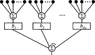
Figure 2.52. Linear array with uniform element weights and weights at the subarray ports.

where w is a vector containing all the w_n. Substituting the element weights into the equation for the array factor results in the following simplification:

where AF_e is the array factor due to a single uniform subarray and AF_s is the array factor due to subarray weighting alone. Equation (2.107) is the product of a uniform array factor due to the elements in one subarray and the array factor due to the weighted sum of isotropic point sources at the phase centers of all the subarrays. Usually, dN_e > λ, so grating lobes appear in AF_s at [21]

Since AF_e has nulls at the same angles as the grating lobes appear, the grating lobes have nulls in their centers. As a result, the grating lobes do not get as large as those associated with large element spacing. An approximate expression for the grating lobe heights relative to the peak of the main beam is [21]

where B_b ≥ 1 is the beam broadening factor (the ratio of the 3-dB beamwidth of the weighted array to the 3-dB beamwidth of the corresponding uniform array). In general, decreasing the sidelobe level increases B_b, which in turn increases the grating lobe heights.

A 64-element array divided into 8 subarrays with a low-sidelobe taper applied to its subarray ports has the effective element weights shown in Figure 2.53. AF_e is the broad beam uniform array factor in Figure 2.54. AF_s has low sidelobes due to the subarray weights and grating lobes due to dN_e > λ. Multiplying these patterns results in the array factor shown in Figure 2.55. Except at u = 0, the peaks of AF_s occur at the nulls of AF_e. The nulls in AF_e place nulls in the grating lobe peaks. These nulls reduce the grating lobes but do not eliminate them.

Example. A 128-element array with d = 0.5λ, can be divided into several different subarray configurations. Table 2.5 shows four possible divisions with their associated maximum grating lobe locations and approximate heights when a low-sidelobe amplitude taper is applied at the subarray ports. This amplitude taper has a beam broadening factor of B_b = 1.288. Increasing the number of elements in a subarray causes the grating lobe to get larger and move closer to the main beam as indicated in Table 2.5.

Figure 2.53. Effective element weights for a 64-element array divided into 8 subarrays with a low-sidelobe taper applied to its subarray ports.

Figure 2.54. Graphs of AF_e, (dashed line) and AF_s, (solid line).

The beam broadening factor is a function of the subarray weighting. For most practical cases, a low-sidelobe amplitude tape will have a higher B_b than a high-sidelobe amplitude taper. B_b has a lower bound of one. Thus, there is some tradeoff between the lowest design sidelobe level and the highest grating lobe level. A higher taper efficiency leads to a lower B_b, which in turn results in a lower peak grating lobe. As a result, optimizing the amplitude taper should lead to a peak sidelobe level that is the same height as the peak grating lobe. One can only expect a small improvement to the maximum sidelobe level through optimization, since increasing B_b to get lower sidelobes also causes the peak grating lobe to increase.

Figure 2.55. Array factor due to the subarray amplitude taper in Figure 2.53.

TABLE 2.5. Some Possible Subarray Divisions of a 128-Element Array and the Location and Approximate Height of the First Grating Lobe

Steering the main beam using phase shifters at the subarray ports results in very large grating lobes. The array factors shown in Figure 2.56 compare steering the pattern in Figure 2.55 to u = 0.12 using phase shifters at the subarray ports only (solid line) and phase shifters at the individual elements (dashed line). Steering AF_s moves the peak of its pattern out of the null of AF_e (which is not steered). These nulls in AF_e are what cause the grating lobes to have a split down the middle in Figure 2.55. Without the nulls in the center of the grating lobes, the grating lobes dramatically increase. Practical beam steering is done at the element level.

2.12. ERRORS

The signals at each element in the array have errors due to manufacturing tolerances, element failures, aging, and quantization. Errors are either modeled as statistically independent from element to element or statistically independent between groups of elements. The main concern with errors is the rise in the sidelobe levels. Other problems include beam pointing errors, loss in gain, and need for recalibration.

Figure 2.56. Comparison between phase steering at the subarray ports (solid line) and phase steering at the element level (dashed line) when the patterns are steered to u = 0.12.

2.12.1. Random Errors

Random errors are statistically independent from element to element. These errors occur within individual array elements and associated components and have no effect on surrounding elements. For the most part, four types of random errors are possible:

1. Random amplitude error,
2. Random phase error,
3. Random position error,
4. Random element failure,

Random amplitude and phase errors appear in the signal weighting while the position errors appear in the relative element phases. An array factor with errors can be written as

If the position and phase errors are relatively small, then the small phase approximation can be used (e^jx ≃ 1 + jx for x 1) for the phase terms in (2.110):

Multiplying the quantities in (2.111) and collecting terms results in

Note that the first summation is the array factor with no errors. The second summation is an error array factor that is added to the array factor with no errors. Since the errors are assumed to be small, all terms that consist of the product of at least two errors can be dropped, leaving

where AF₀ is the error free array factor.

The error pattern effects are easy to see at a null in the error-free array factor, because the error-free pattern is zero and only the error term in (2.113) remains. In order to analyze the contribution of each type of error, assume that only one error at a time exists. The power pattern due to the amplitude weights alone is proportional to the magnitude of the error array factor squared.

Taking the average value of the power pattern (line over quantity) results in

Similar average power patterns occur for the other two error types:

Since is just as likely to add as to subtract from the main beam, it does not change the peak value of AF but has a relatively constant effect in the sidelobe region. Thus, the relative sidelobe level caused by the amplitude errors is the ratio of the sidelobe power to the power in the peak of the main beam:

On the other hand, the phase errors cause small subtractions from the main beam as well as produce a relatively constant pattern in the sidelobe region. As a result, the average sidelobe level due to random phase errors is given by

The relative sidelobe level due to position errors alone is

Position errors have little effect in the main beam region (u is very small) but have an increasing effect toward u = ±1.

Example. A 50-element linear array (d = 0.5λ) has a low-sidelobe taper. Plot AF_amperr, AF_pherr, and AF_poserr when , and .

Figure 2.57 shows the plots. Random amplitude and phase errors have approximately the same magnitude over all the angles, while the position errors increase with |u|.

A different type of random error occurs when elements stop functioning. Element failures result from amplifier, receiver, phase shifter, and so on, malfunctions. The peak of the main beam is now at Nη_tP^e, where P^e is the probability of element failure. Assuming that the element failures are uniformly distributed across the aperture, the formula for rms sidelobe levels due to failed elements is

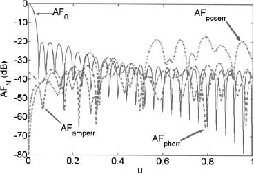
Figure 2.57. Plot of AF_amperr (dashed line), AF_pherr (dash-dot line), and AF_poserr (dotted line) when and . The error-free pattern is the solid line.

Comparing this formula with (2.118) reveals that the probability that an element has failed, 1−P_e, is the same as an rms amplitude error, . Position errors are relatively small compared to the other three errors, so a formula to calculate the rms sidelobe level of the array factor for amplitude and phase errors with element failures is [22]

Example. A 30-element linear array (d = 0.5λ) has a 30-dB, = 7 low-sidelobe taper. Show the effects of a single element failure at (1) the edge and (2) the center of the array.

Figure 2.58 shows the array factors superimposed on each other. Since the edge element has a low amplitude, it has little effect on the pattern when it fails. When the center element fails, the sidelobes significantly increase. The original pattern has η_T = 0.8535, while the edge failed taper has η_T = 0.8332 and the center element failed taper has η_T = 0.8243.

So far, only random, uncorrelated errors have been mentioned. If the same error occurs for groups of elements, then that error is correlated within that group of elements even though the error is random. An example would be a random amplitude error at the subarray port. That random error is passed on to each element in the subarray, so it is the same for all the elements of that subarray; hence there is a correlated error between elements of that subarray.

Figure 2.58. Array factor of a 30-element linear array (d = 0.5λ) with a 30 dB, = 7 low-sidelobe taper (dotted line) superimposed on the same array factor with element 1 failed (solid line) and element 15 failed (dashed line).

Figure 2.59. Array factor of a 36-element linear array (d = 0.5λ)with a low-sidelobe taper (dotted line) and divided into 6 subarrays of 6-elements each. The dashed line in the pattern with random errors at the subarray ports only ( and ). Plots of AF_amperr (solid line) and AF_pherr (dash-dot line) are superimposed.

Example. A 30-element linear array (d = 0.5λ) has a 20-dB, = 2 taper applied at the elements. The array is divided into 6 subarrays, each having 6 elements. Plot the error patterns when 0.1 and at the subarray port.

Figure 2.59 has graphs of the array factor with no errors, with both the phase and amplitude errors, and AF_amperr and AF_pherr. The errors have greatest impact at the grating lobe locations.

2.12.2. Quantization Errors

Phase shifters and attenuators have digital controls with a finite number of possible values. For instance, the least significant bit associated with amplitude and phase have the following values:

where N_ba is the number of amplitude bits and N_bp is the number of phase bits. A quantized amplitude weight has the value of

and the quantized phase has a value of

where floor rounds down to the closest integer. If only the phase steering is quantized, then δ_n is not included in this equation.

If the difference between the desired and quantized amplitude weight is assumed to be a uniformly distributed random number with the bounds being the maximum amplitude error of , then the rms amplitude error is . This value can then be substituted into (2.122) to find the rms sidelobe level.

If no two adjacent elements receive the same quantized phase shift, then the difference between the desired and quantized phase shifts are treated as uniform random variables between . As with the amplitude error, the random phase error formula in this case is . These same quantized phase errors result in beam-pointing errors too. The difference in phase between the desired and quantized steering phase shifts is

Solving for the angular difference at element n yields

Taking the average value of the right-hand side of (2.128) for all the elements in the array and the rms quantization error leaves

Either increasing the number of bits in the phase shifters or increasing the aperture size reduces the beam pointing error.

When two or more elements have the same quantized phase shift, then the error is correlated and quantization lobes form. This situation occurs when the beam is steered to a small angle off boresite. The maximum phase shift across an aperture is given by

The total number of elements that receive the same quantized phase shift is then

This means that there are N/N_Q subarrays of N_Q elements that receive the same phase shift. The grating lobes due to these subarrays occur at [21]

The approximation in (2.132) assumes the array has many elements. For large scan angles, quantization lobes do not form, because the element-to-element phase difference appears random. The relative peaks of the quantization lobes are given by [21]

Figure 2.60 shows a low-sidelobe array factor for a 10-element, d = 0.5λ array with its beam steered to u = 0.1 when the phase shifters have 3, 4, and 5 bits.

Example. Find the location and heights of the quantization lobes for a 10-element array with d = 0.5λ and the beam steered to u_s = 0.05 when the phase shifters have 3, 4, and 5 bits.

The location and heights of the grating lobes are calculated from (2.132) and (2.133).

Figure 2.60. Array factors steered to u = 0.1 when there are 3-, 4-, and 5-bit phase shifters.

There are no grating lobes for the 5-bit phase shifters. The location of the grating lobes and their heights are only approximate. The actual values calculated from the array factor are given by

Phase dithering reduces the size of the quantization lobes by adding a random phase to each phase shifter [23]. For large arrays, this random phase has very little impact on the main beam-pointing angle. Two other similar approaches that breakup correlated errors with small random errors include frequency and beam dithering [23].

2.13. FRACTAL ARRAYS

A fractal is a self-similar shape with a non-integer dimension [24]. Self-similar means that a magnified portion of the shape has the same structure as the whole geometry. Fractals were first applied to antenna arrays by Kim and Jaggard [25]; and since then, several analysis and synthesis techniques for fractal arrays have been developed [26,27].

Fractal arrays can be formed through recursive application of a generating array used to create the much larger self similar array. The generating array has a pattern that is copied, scaled, and translated many times. There are a total of N_G elements in the generating array with N₁ of the elements having an amplitude of one and the rest having an amplitude of zero. An example is the Cantor array [28] that has a 3-element (N_G = 3) generating array with weights given by

The next scale is found by replacing a 1 with 101 and replacing a 0 with 000.

Applying the formula to obtain the next scale yields

Although this array does not have practical use, it does have some interesting properties. For instance, the array factor can be expressed as a product rather than a sum:

where AF_G is the array factor of the generating array. If d = 0.25λ, then the closest that two elements are spaced in the thinned aperture is 0.5λ, so the directivity is derived from (2.68)

The generating array for Cantor arrays with every other element having an amplitude of zero may be expressed in the form

Other versions of the generating array are also possible. For instance, N_G = 5 has the weighting

The recursive building of larger arrays results in much different array weights. Proceeding to the second scale results in the weights

which differs from either (2.135) or (2.136).

The fractal array factor is based upon an iterated (recursive) function. Therefore, the array factor can be calculated via the product of S generating array factors rather than the N additions and multiplications in a normal Fourier series representation of the array factor.

The fractal dimension D of these Cantor arrays are calculated using [28]

which results in f_dim = 0.6309 for N_G = 3, f_dim = 0.6826 for N_G = 5, and f_dim = 0.7124 for N_G = 7.

Example. Plot the array factors for the first four scales of the Cantor array when the generating array has d = 0.25λ.

The array factor of the three-element generating array is

where ψ = πu. An expression for the normalized Cantor array factor given by

Figure 2.61. Array factors for N_G = 3 and S = 1,2, 3,4.

Figure 2.62. Array factors for N_G = 3 and S = 5.

The array factors for S = 1,2,3, and 4 are shown in Figure 2.61. You can see how similar the shape of the array factor are. Figure 2.62 shows the array factor at S = 7.

A Sierpinski carpet is a two-dimensional version of the Cantor set [29]. An example of a generating array on a square lattice is

1  1  1
1  0  1
1  1  1

The normalized array factor associated with this generating subarray for d_x = d_y = λ/2 is given by

The expression for the fractal array factor at stage S is

The geometry for this Sierpinski carpet fractal array at progressive stages of growth appears in Figure 2.63 along with a plot of the corresponding array factors. The array factors look self-similar.

Linear polyfractal arrays can exhibit ultra-wideband characteristics when numerically optimized [30]. Polyfractal arrays are constructed from a set of multiple generatoring arrays rather than a single generating array. A 32-element linear polyfractal array was designed and built to have a wide bandwidth with suppressed grating lobes and relatively low sidelobes (−16.3 dB at f₀ and −5.39 dB at 4f₀). The 32-element array was divided into 4 subarrays of 8 elements each as shown in Figure 2.64. Each subarray pattern was calculated and measured then coherently combined to find the array pattern of the 32 element array. Figure 2.65 shows the close agreement between the calculated and measured patterns.

Figure 2.63. Sierpinski carpet array and associated array factors for the first three stages.

Figure 2.64. Sierpinski carpet array and associated array factors for the first three. (Courtesy of Douglas Werner, Pennsylvania State University.)

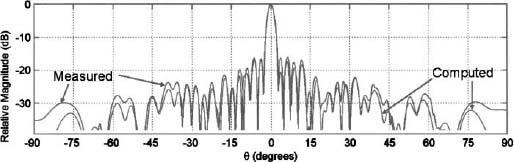
Figure 2.65. Sierpinski carpet array and associated array factors for the first three. (Courtesy of Douglas Werner, Pennsylvania State University.)

REFERENCES

1. R. J. Mailloux, Phased Array Antenna Handbook 2^nd ed., Norwood, MA: Artech House, 1994.
2. W. W Hansen and J. R. Woodyard, A new principle in directional antenna design, Proc. IRE, Vol. 26, No. 3, March 1938, pp. 333–345.
3. W. K. Bartley, Near-field antenna focussing, Goddard Space Flight Center Report X-811-75-183, Greenbelt, MD, August 75.
4. A. J. Fenn, C. J. Diederich, and P. R. Stauffer, An adaptive-focusing algorithm for a microwave planar phased-array hyperthermia system, Lincoln Lab. J., Vol. 6, No. 2, 1993, pp. 269–288.
5. L. J. Ricardi and R. C. Hansen, Comparison of Line and Square Source Near-Fields, Trans. IEEE, Vol. AP-11, November. 1963, pp. 711–712.
6. R. C. Hansen, Minimum spot size of focused apertures, URSI Symposium on EM Theory, Delft: Pergamon, Press, 1965, pp. 661–667.
7. E. Sharp, A triangular arrangement of planar-array elements that reduces the number needed, IRE AP-S Trans., Vol. 9, No. 2, 1961, pp. 126–129.
8. J. Hsiao, Properties of a nonisosceles triangular grid planar phased array, IEEE AP-S Trans., Vol. 20, No. 4, 1972, pp. 415–421.
9. R. J. Mailloux et al., Multiple mode control of grating lobes, RADC Technical Report 76–307, September 1976.
10. L. Corey, J. Weed, and T. Speake, Modeling triangularly packed array antennas using a hexagonal FFT, IEEE AP-S Symp., June 1984, pp. 507–510.
11. S. Silver, Aperture illumination and antenna patterns, in Microwave Antenna Theory and Design, London: Peter Peregrinus, 1949, pp. 169–199.
12. S. A. Schelkunoff, A mathematical theory of linear arrays, Bell Syst. Tech. J., Vol. 22, 1943, pp. 80–107.
13. C. A. Balanis, Antenna Theory Analysis and Design, 2nd ed., New York: John Wiley & Sons, 1997.
14. C. Steams and A. Stewart, An investigation of concentric ring antennas with low sidelobes, IEEE AP-S Trans., Vol 13, No. 6, November 1965, pp. 856–863.
15. R. Das, Concentric ring array, IEEE AP-S Trans., Vol. 14, No. 3, May 1966, pp. 398–400.
16. F. Adcock, Improvement in means for determining the direction of a distant source of electromagnetic radiation, British Patent 1304901919, 1917.
17. E. J. Baghdady, New Developments in Direction-of-Arrival Measurement Based on Adcock Antenna Clusters, Proc. of the IEEE Aerospace and Electronics Conference, Dayton, OH, May 22–26, 1989, pp. 1873–1879.
18. A. Manikas, A. Alexiou, and H. R. Karimi, Comparison of the ultimate direction-finding capabilities of a number of planar array geometries, IEE Proc. Radar, Sonar Navig., Vol. 144, No. 6, December 1997, pp. 321–329.
19. A. Swindlehurst, and T. Kailath, Azimuth/elevation direction finding using regular array geometries, IEEE AES Trans., Vol. 29, No. 1, January 1993, pp. 145–156.
20. R. C. Hansen, Phased Array Antennas, New York: John Wiley & Sons, 1998.
21. R. J. Mailloux, Array grating lobes due to periodic phase, amplitude, and time delay quantization, IEEE AP-S Trans., Vol. 32, December 1984, pp.1364–1368.
22. E. Brookner, Antenna Array Fundamentals—Part 2, in Practical Phased Array Antenna Systems, E. Brookner, ed., Norwood, MA, Artech House, 1991.
23. R. H. Sahmel and R. Manasse, Spatial statistics of instrument-limited angular measurement errors in phased array radars, IEEE Transactions on Antennas and Propagation, Vol. 21, No. 4, July 1973, pp. 524–532.
24. B. B. Mandelbrot, The Fractal Geometry of Nature. New York: W. H. Freeman, 1983.
25. Y. Kim and D. L. Jaggard, The fractal random array, Proc. IEEE, Vol. 74, No. 9, pp. 1278–1280, 1986.
26. D. H. Werner, et al., The theory and design of fractal antenna arrays, in Frontiers in Electromagnetics, D. H. Werner and R. Mittra, eds., New York: John Wiley & Sons, 2000, pp. 94–203.
27. D. H. Werner, R. L. Haupt, and P. L. Werner, Fractal antenna engineering: The theory and design of fractal antenna arrays, IEEE Antennas Propagat. Mag., Vol. 41, No. 5, October 99, pp. 1009–1015.
28. C. Puente Baliarda and R. Pous, Fractal design of multiband and low side-lobe arrays, IEEE Trans. Antennas Propagat, Vol. 44, No. 5, pp. 730–739, May 1996.
29. H. O. Peitgen, H. Jurgens and D. Saupe, Chaos and Fractals: New Frontiers of Science, New York: Springer-Verlag, 1992.
30. J. S. Petko, and D. H. Werner, The Pareto optimization of ultrawideband polyfractal arrays, IEEE AP-S Trans., Vol. 56, No. 1, pp. 97–107, January 2008.