5 Nonplanar Arrays

Array elements usually lie in a plane, because the feed network for nonplanar array is more complicated. In addition, placing array elements on a curved surface complicates design, construction, and testing. A nonplanar array, like the one in Figure 5.1, with elements distributed in three-dimensional space has an array factor given by

where

A conformal array has the (x_n, y_n, z_n) lying on a curved surface. The maximum gain of a conformal array equals the sum of the array element gain pattern values in the main beam direction when they are phase compensated. This chapter presents a number of approaches to distributed and conformal array configurations.

5.1. ARRAYS WITH MULTIPLE PLANAR FACES

Linear and planar arrays have limited scan regions due to element patterns, mutual coupling, and grating lobes. One way to increase the array scanning region uses multiple linear/planar arrays that face in different directions. Each planar array lies on a side of a three-dimensional polygon surfaces [1], Figure 5.2 shows some polygons with faces that can accommodate arrays for complete azimuth scanning. A 360° azimuth scan requires that each array face equally divides the azimuth for scanning. As a result, one face has an azimuth scan defined by

Figure 5.1. Arbitrary distribution of elements in the x–y plane.

Figure 5.2. Three-dimensional polygonal surfaces for full azimuth scanning.

where N_p are the number of sides to the polygon. The size of one face of the polygon is determined by the required gain and beam width.

PAVE (Precision Acquisition Vehicle Entry) PAWS (Phased Array Warning System) (AN/FPS-115) is a UHF array built by Raytheon in 1978 to detect and track sea-launched ballistic missiles (Figure 5.3) [2]. It has two faces inclined 120° to each other with 1792 T/R (transmit/receive) modules (per face) connected to dipole radiating elements that operate from 420 to 450 MHz. Each element has a 4-bit phase shifter. The modules are grouped into 56 subarrays of 32 elements. The receive antenna gain is 34 dB.

Figure 5.3. PAVE PAWS (AN/FPS-115) array. (Courtesy of the National Electronics Museum.)

Figure 5.4. MESA array with installation on a Boeing 737 in the lower right corner. (Courtesy of Northrop Grumman and available at the National Electronics Museum.)

The multirole electronically scanned array (MESA) is a different multiple face array concept that provides 360° coverage on a Boeing 737 without rotating the antenna (Figure 5.4). The MESA antenna (called the Wedgetail) has three electronically scanning arrays that share 288 L-band T/R modules [3]. The port and starboard arrays scan ±60°, while the “Top Hat” endfire array provides ±30° front and back scanning as shown in Figure 5.5. The array shape is very aerodynamic, with the “Top Hat” providing additional lift for the airplane.

Figure 5.5. MESA array azimuth scanning.

Figure 5.6. Linear array bent to conform to a circular arc.

5.2. ARRAYS ON SINGLY CURVED SURFACES

Figure 5.6 shows a linear array bent around a circular arc. If the element spacing remains constant along the arc, then the spacing between the elements is approximately equal to

where r_c is the radius of curvature. If the radius of the circular arc is large, then the linear array is only slightly curved; and when r_c = ∞, the arc becomes a straight line. End elements of the conformal arc array are at (r_ccos₁, r_csin ₁) and (r_c cos_N, r_csin_N) when the midpoint of the arc is at(0, r_c). The main beam radiates away from the convex side of the arc or in the +y direction.

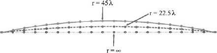
Figure 5.7. Conformal linear array with r_c = ∞, 45λ, and 22.5λ.

Figure 5.8. Array factors for uniformly weighted conformal linear arrays with r_c = ∞, 45λ, and 22.5λ.

As r_c decreases, the array curvature increases, and the changes to the array factor become more dramatic. For instance, r_c values of ∞, 45λ, and 22.5λ produce the array bends shown in Figure 5.7. If the array has uniform weighting, then the resulting array factors appear in Figure 5.8. The directivity decreases from 13.0 to 11.8 to 8.0 dB as the curvature decreases from ∞ to 45λ to 22.5λ. Relative sidelobe levels near the main beam rise from 13.3 to 8.3 to 0.8 dB, but the sidelobes far from the main beam exhibit little change. Figure 5.9 shows the array factors associated with Figure 5.7 when the weighting is a 25 dB Taylor = 5 amplitude taper. In this case, the directivity decreases from 12.6 to 11.7 to 9.2dB. This decrease in directivity is less than that of the corresponding uniform array, because the end elements that are most displaced from the center have the lowest amplitude. Again, the pattern within ±45° of the main beam is distorted, while the sidelobes beyond that range are not. The distortion in this case is in the form of the first sidelobe (r_c = 45λ) and first two sidelobes (r_c = 22.5λ) being absorbed into the main beam.

Curvature compensation restores the array factor to the desired array factor by applying a phase shift, δ_n, that offsets the y translation.

Figure 5.9. Array factors for 25-dB Taylor = 5 weighted conformal linear arrays with r_c = ∞, 45λ, and 22.5λ.

Figure 5.10. Compensated array factor for a 25-dB Taylor = 5 weighted conformal linear arrays with r_c = 11.1λ.

where the main beam is steered to _s. This equation implies that the phase compensation changes at each scan angle and is independent of the amplitude taper. Applying (5.4) to the array factor of a 20-element d = 0.5λ spaced array having r_c = 11.1λ with a 25-dB Taylor = 5 results in the array factor shown in Figure 5.10. The compensation restores the main beam and sidelobes to the desired levels. The directivity increases from 6.2 to 12.5 dB (which is the same as the corresponding linear array with r_c = ∞), and the maximum sidelobe level is 23.3 dB below the peak of the main beam. Since the array has a smaller extent in the x direction, the array factor for the curved array array factor has the number of sidelobes of a linear array factor that is 2x_c long.

Figure 5.11. Compensated array factor for a 25-dB Taylor = 5 weighted conformal linear arrays with r_c = 11.1λ. when the main beam points at _s = 120°.

Example. Graph the array factor for a 25-dB Taylor = 5 weighted conformal linear arrays with r_c = 11.1λ when the main beam points at _s = 120°.

Figure 5.11 shows the compensated array factor superimposed on the r_c = ∞ array factor. The sidelobe peaks at angles greater than about 100° increased between 2 and 7dB, while the rest of the sidelobes look like those of the desired pattern.

The phase correction in (5.4) works well to restore the pattern of a linear or planar array conforming to the surface of a curved surface like a cylinder. Finding the weights that produce a more complicated pattern, such as a flat-top main beam, requires numerical methods to adjust either the amplitude and phase [4-6] or phase alone [7].

In almost all conformal antennas, the element pattern peak is normal to the surface, so the peaks will not all point in the same direction as with linear and planar arrays. Figure 5.12 is a diagram of a conformal array displaying both isotropic and directional element patterns. The isotropic element patterns all contribute the same amplitude in a given direction, while the directional element patterns do not. Since the element pattern is a different function of for each element, the element pattern remains inside the sum sign of the array factor.

Figure 5.12. Comparison of a conformal array with directional elements to one with isotropic elements.

where e( − _n) is the element pattern of element n having a peak at = 0°. Now, the antenna pattern is not the product of a single element pattern times an array factor.

As with a linear array, the directivity and sidelobe level changes when including the element patterns. Typically, the element pattern maximum points normal to the surface where the element lies. The antenna pattern changes when the peaks of all the element patterns point toward 90°. In this case, the antenna pattern is the product of the element pattern and the array factor. Consider a 20-element array with elements spaced λ/2 over an arc of radius 11.1λ. If the peak of the element patterns point normal to the arc, then the element patterns are represented by

When all the element pattern peaks point toward 90°, then _n = 90°. Figure 5.13 shows little difference between the antenna patterns of the array with the elements pointing normal and the elements pointing 90° except for angles far from the main beam. Figure 5.14 shows the beam steered to 25° off boresight for the array with _n = 90°. The directivity decreases from 22.7 to 21.9 dB, while the relative sidelobe level increases about 2 dB.

Figure 5.13. Comparing the antenna patterns of two conformal arrays. One has the maximum element patterns normal to the surface while the other has the element pattern peaks pointing to = 90°.

Figure 5.14. Main beam of the conformal array steered to = 65°.

A polar plot of all the element patterns for a 10-element array appears in Figure 5.15. Dotted lines indicate the directions of the element pattern peaks. It is easy to see that the element pattern of element 1 contributes little field in the direction of the maximum of element pattern 10.

Figure 5.15. Polar plot of all the element patterns for a 10-element conformal array when their peaks point normal to the surface.

Figure 5.16. Linear array bent at an angle of 45°.

Example. A uniformly weighted 20-element linear array with element spacing of 0.5λ is bent at an angle of 90° as shown in Figure 5.16. Plot the uncompensated array factor, the compensated array factor, the antenna pattern with element patterns pointing in the direction of the normal to the surface, and the antenna pattern steered to 67.5° and 45°.

The uncompensated pattern has a directivity of −15.1 dB at = 90° with large 13-dB lobes at 45.5° and 135°. Phase compensation restores the directivity at = 90° to 16 dB. The large lobes are reduced to 12.6 dB and move to 28° and 152° These patterns are shown in Figure 5.17. The compensated antenna pattern when all the element pattern peaks point toward = 90° is shown in Figure 5.18. Now, the main beam has a directivity of 19.2 dB. Large lobes at 28° and 152° have a directivity of only 6.6 dB. Figure 5.19 shows the compensated antenna pattern steered to 67.5° and 45°. The main beam directivity is 15.4 dB at 67.5° and 13 dB at 45°.

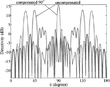
Figure 5.17. Compensated and uncompensated antenna patterns for the array in Figure 5.16.

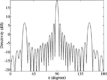
Figure 5.18. Antenna pattern when the peaks of the elements point toward = 90° for the array in Figure 5.16.

Figure 5.19. Steering the compensated antenna pattern in Figure 17 to 67.5° and 45° when _n = 90°.

A Wullenweber antenna [8] is a large direction finding circular array with a narrow beam that scans 360° in azimuth. Only a small group (N_wul) of adjacent elements are active at a time with the array factor

where N_wul < N. The main beam points normal to the center of that group of elements. A commutating feed connects the active elements to the output (Figure 5.20). As the commutating feed rotates, the group of active elements changes by one element, and the main beam points in a new azimuth direction. Phase compensation is only applied to the active elements. To form a coherent beam in the desired direction _s, the element weights in (5.7) are given by

A 60-element Wullenweber array with 0.5λ spacing between elements is shown in Figure 5.20 when the indicated 15 elements (large dark dots on the center circle) are turned on. Its corresponding array factor is shown in Figure 5.21.

The Wullenwever array was invented during World War II by Dr. Hans Rindfleisch [9], The name Wullenwever was a World War II German cover name for the antenna and not the name of a person. The first one, which was built in Skisby, Denmark, used 40 vertical radiator elements, placed on a 120-m-diameter circle with 40 reflecting elements installed behind the radiator elements around a circle having a diameter of 112.5 m. After the war, the Soviet Union imported the technology and built many Wullenwevers for HF direction finding, which included tracking Sputnik. The United States became interested in the technology in the late 1950s and early 1960s. At some point, the Americans changed the name from Wullenwever to Wullenweber. Its immense size and huge circular reflecting screen inspired such names as “elephant cage” and “dinosaur cage.” The University of Illinois built a large Wullenweber array with 120 monopoles over 2 to 20 MHz. Tall wooden poles supported a 1000-ft-diameter circular screen of vertical wires located within the ring of monopoles. In 1959 the Navy began construction of the AN/FRD-10 HF/DF arrays which were based on the experimental investigations at the University of Illinois. The FRD-10 had two concentric rings: The high-frequency array was 260 m in diameter with 120 sleeve monopoles, while the low-frequency array was 230 m in diameter with 40 folded dipoles. Inside each ring there was also a large wire screen, supported by 80 towers. AN/FLR-9 Wullenweber antenna array near Augsburg, Germany is shown in Figure 5.22.

Figure 5.20. Diagram of a Wullenweber array.

Figure 5.21. A 60-element Wullenweber array with 15 elements turned on (large dark dots on center circle) and its array factor.

Figure 5.22. AN/FLR-9 Wullenweber antenna array near Augsburg, Germany.

5.2.1. Circular Adcock Array

An Adcock array [10] with many elements arranged in a circle [11] was introduced in Chapter 4. Table 5.1 shows how the signals from adjacent elements combine to form four beams. Opposite beams form difference patterns as with the standard 4-element Adcock array. Subtract beam 3 from beam 1 to get

Subtract beam 4 from beam 2 to get

TABLE 5.1. Element Signals and Beams Formed by the 8-Element Adcock Array

The phase at element n is given by

An omnidirectional pattern results from the sum of the signals from all the elements

which for this array is

Example. Design an 8-element Adcock array that works at 1GHz (Figure 5.23). Show the effects of increasing frequency.

Start with a circular array that has a radius of 7.5 cm. The sum, difference, and omni patterns at 1 GHz are shown in Figure 5.24. Increasing the frequency to 1.5-GHz results in the patterns shown in Figure 5.25. At this point, the diameter of the circle is 0.75λ and sidelobes are beginning to form. The effect of frequency on the direction capability is demonstrated in Figure 5.26. At the design frequency of 1 GHz, the calculated and actual directions are very close. There are small deviations at 1.5 GHz. At 2.0 GHz the error is so large that the array can only tell if the signal comes from 0°, 90°, 180°, or 270°.

Figure 5.23. Diagram of an 8-element Adcock array.

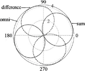
Figure 5.24. Sum (solid), difference (dashed), and omni- (dotted) array factors for the 8-element Adcock array at 1 GHz

Figure 5.27 is an example of a linear array of z-directed dipoles wrapped around a cylinder that is a perfect electrical conductor (PEC). The element field of view extends ±(90° + γ), where γ = cos⁻¹(r_c/(r_c + h)). Consider an array located in the x−y plane with half wavelength dipoles placed h = λ/4 away from the perfectly conducting cylinder that is 2λ in diameter and 2λ tall (Figure 5.28). Elements are spaced λ/2 apart in arc length. The field of view for an element in this array is 234.5°. An element can see up to four other elements to its left or right, while the rest are not in its line of sight. Figure 5.29 are the directivity plots for phase compensated arrays with 1, 3, and 5 elements. A single element has a directivity of 7.1 dB, while 3 and 5 elements are 10.9 dB and 13.1 dB, respectively. Blockage is not an issue for these small arrays. Increasing the number of elements to 11 does block the elements on one end of the array from “seeing” the elements on the other end. If the 11-element array is not phase compensated, then the directivity is 7.0 dB. Compensation improved the directivity to 16.2 dB as shown in Figure 5.30. Letting _s = 60° and applying the phase shift from (5.4) results in the array pattern in Figure 5.31. The actual peak of the beam is at = 58°, where the directivity is 14.4dB. The directivity at = 60° is 14.16 dB.

Figure 5.25. Sum (solid), difference (dashed), and omni- (dotted) array factors for the 8-element Adcock array at 1.5 GHz.

Figure 5.26. Graph of the calculated versus actual azimuth angle for the 8-element Adcock array at three different frequencies.

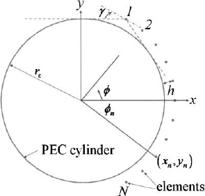
Figure 5.27. Top view of dipole array with cylindrical ground plane.

Figure 5.28. Three-dimensional diagram of dipole array conformal to a perfectly conducting cylinder.

Figure 5.29. Directivity of an array of dipoles on a perfectly conducting cylinder with N = 1, 3, and 5 elements.

Figure 5.30. Directivity of an 11-element array of dipoles on a perfectly conducting cylinder when phase is compensated and uncompensated.

Figure 5.32 shows an array of spirals wrapped around the center of an ellipsoid-shaped airship [12]. This array operates from 800 to 1200MHz. The elements are two-arm, self-complementary Archimedean spirals, 12.5 cm in diameter. The microstrip spiral element was etched on a 0.8-mm-thick, ε_r = 3.38 substrate. The spiral is unbalanced and has an input impedance of 188Ω, so a surface mount transformer is used as a balun and a match to the 50-Ω coax. In this case, the curvature is not uniform but is a function of the location on the ellipsoid surface. Figure 5.33 shows the measured and computed uncompensated array patterns of an 8-element array on the front of the airship with a 20° radius of curvature. Figure 5.34 shows the measured and computed uncompensated array patterns of an 8-element array when the side of the airship has a 5° radius of curvature. The pattern of the side array has a distinct main beam, while the front array does not.

Figure 5.31. Compensated main beam steered to _s = 0° (dashed line) and _s = 60° (solid line).

Figure 5.32. Airship with conformal array of spiral antennas. (Courtesy of Régis Guinvarc’h, SONDRA, Supelec.)

Figure 5.33. Calculated and measured antenna patterns for a 20° radius of curvature (front). (Courtesy of Régis Guinvarc’h, SONDRA, Supelec.)

Figure 5.34. Calculated and measured antenna patterns for a 5° radius of curvature (side). (Courtesy of Régis Guinvarc’h, SONDRA, Supelec.)

AIRLINK^® is an airborne antenna system for in-flight telephone, fax, and data transmission that uses the INMARSAT (International Maritime Satellite) system of geostationary satellites. The antenna array is very thin and curved (Figure 5.35) to conform to the outside of an airplane. Figure 5.36 shows the array being installed on the outside of an airplane. The array operates at 1530 to 1559 MHz on receive and 1626.5 to 1660.5 MHz on transmit. It has a gain of greater than 12 dB with a VSWR of less than 1.5. Figure 5.37 is a picture of the Airlink array with rectangular microstrip elements that are spaced half a wavelength (9.27 cm) apart on a triangular grid. The array is capable of scanning ±60° in azimuth and elevation.

Figure 5.35. Front and side views of the Airlink antenna. (Courtesy of Ball Aerospace & Technologies Corp.)

Figure 5.36. Airlink antenna being installed on an airplane (Courtesy of Ball Aerospace & Technologies Corp.)

Figure 5.38 is an artist concept of a multilayer conformal array antenna showing installation on curved surface. A thin dielectric covering protects the crossed bow-tie elements from the environment. The output from the element is fed to a phase shifter mounted below the surface. Low-dielectric-constant foam supports the elements above the ground plane. Elements are placed in subarrays as shown by the small rectangular portions of the array.

Figure 5.37. Airlink array elements. (Courtesy of Ball Aerospace & Technologies Corp.)

Figure 5.38. Multilayer conformal array antenna. (Courtesy of the National Electronics Museum.)

5.3. ARRAYS CONFORMAL TO DOUBLY CURVED SURFACES

Arrays that conform to doubly curved surfaces are relatively rare, because they are difficult to build. A doubly curved surface has curvature in two orthogonal directions. The spherical array is the most common type of conformal array on a doubly curved surface. A spherical array of point sources has an array factor given by (5.1). Assume that the elements are placed in rings that are conformal to the sphere with a center element at (0, 0, 0). Element m in ring n on a sphere of radius r are located at (x_mn, y_mn, z_mn), where

The function floor rounds down to the nearest integer. The phase compensation must be applied to the elements in the form

Example. Plot the uncompensated and compensated far-field patterns of a 5-ring array placed on a sphere of radius 4λ. Assume d_θ = 0.5λ and d_desired = 0.5λ.

First, the values of d, N_n, and r_n are found and displayed in Table 5.2. Next, the element locations are calculated and shown on the sphere in Figure 5.39. The array factor is calculated using (5.1) and shown in Figure 5.39 as the uncompensated pattern. The phase compensation is just δ_mn = −kz_mn. The compensated pattern is shown in Figure 5.39.

TABLE 5.2. List of Spherical Array Variables

Figure 5.39. Uncompensated and compensated array factors for the 5-ring array paced on a sphere.

The previous example used isotropic point sources, with no mutual coupling, no ground plane, no element patterns, and no blockage. A more realistic example includes all these factors. Assume a spherical array of dipoles that are 0.48λ long and 0.25λ above a perfectly conducting partial sphere that has a radius of 4λ. Figure 5.40 shows a 3-ring array above a 30° sphere section with its uncompensated and compensated far-field patterns. The partial sphere angle is defined as the angle between the radius to the center of the partial sphere and the radius to the edge of the partial sphere. The uncompensated gain of 17.7 dB increases to 20 dB with phase compensation. Increasing the size of the partial sphere to 45° produces little change to the compensated pattern that now has a gain of 20.3 dB, but decreases the uncompensated pattern gain to 14.7dB (Figure 5.41). Increasing the number of rings on the 45° sphere to 5 results in the array with uncompensated and compensated patterns shown in Figure 5.42. The gain of the uncompensated pattern is 12.8 dB, and the gain of the compensated pattern is 23.4dB. As more rings are added, the main beam of the uncompensated pattern gets worse because the z distance of each additional ring gets larger. Steering the beam from 0° to 60° in 15° increments is shown in Figure 5.43 for = 0. The gain decreases from 23.4 dB at 0° to 20.9dB at 60°.

As with a circular array, usually only a subsection of a spherical array is active at a time. The feed network dynamically connects to the appropriate elements to form an aperture on a portion of the sphere that faces the direction of the desired main beam location. The active elements on the sphere are contained within a cone having an apex at the origin, a cone half-angle of α_max, and the main beam pointing perpendicular to its base. Figure 5.44 shows the circular boundary of active elements on the sphere. The arrow from the origin through the center of the base points in the direction of the main beam. Thus, the array has a circular boundary. This implementation has many advantages over a multifaced array [13]:

Figure 5.40. Three-ring array of dipoles placed λ/4 above a perfectly conducting portion of a 30° sphere with uncompensated and compensated far-field patterns.

Figure 5.41. Three-ring array of dipoles placed λ/4 above a perfectly conducting portion of a 45° sphere with uncompensated and compensated far-field patterns.

Figure 5.42. Five-ring array of dipoles placed λ/4 above a perfectly conducting portion of a 45° sphere with uncompensated and compensated far-field patterns.

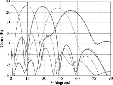
Figure 5.43. Array pattern in Figure 5.42 steered to = 0° and θ = 0° to 60° in 15° increments.

Figure 5.44. Cone for spherical array.

1. Lower polarization losses.
2. Lower mismatch losses.
3. No beam shift versus frequency (implies wider bandwidth).
4. No gain loss with beam steering.

Planar arrays usually cannot scan beyond about 60°, giving spherical arrays a significant advantage. The radiating elements in the active sector are assumed to have symmetry in the plane perpendicular to the axis of the antenna beam, and consequently a spherical array can be used to cover the hemisphere with practically identical beams. Thus, in contrast to other array configurations which suffer from beam degradation as the beam is steered over wide angular regions, spherical arrays provide uniform patterns and gain over the entire field of view. Fabrication and assembly of the curved radiators and feed network is challenging.

The gain of the spherical array is based on its projected aperture shown in Figure 5.45.

where the projected area of active sector is

Figure 5.45. Projected aperture of spherical array.

Substituting (5.16) into (5.15) results in [14]

The polarization efficiency of a spherical array is a function of the size of the active area on the sphere [14].

while the planar array polarization efficiency is a function of the scan angle [14].

Example. Compare the polarization efficiencies of a planar array scanned to 60° and a spherical array with α_max = 60°.

The planar array has p = 0.625 and the spherical array has p = 0.809.

The spherical array bandwidth criterion requires the phase difference between the center element and an edge element is less than π/2 as the frequency changes from f₀ to f [14].

If Δf = 2 | f₀ − f |, then (5.20) is written as

This criterion gives about 1-dB loss at the edge of the band.

Example. Compare the bandwidth of a planar array scanned to 60° and a spherical array with α_max = 60°, R = 5m, and f = 2GHz.

Substituting into (5.21) produces Δf/f₀ = 3% or Δf = 60MHz. If the circular planar array has a radius of R sin α_max = 4.33 m, then its beamwidth is 1° with a bandwidth of 1%.

In order to overcome the disadvantages of a spherical array, the sphere approximates a polyhedron (a solid figure with four or more faces). Cheaper planar array technology is then used for panels on the flat faces while the array still approximates a spherical shape. A geodesic sphere is a skeleton of a sphere built using only straight supports that form polygons (most commonly triangles). Figure 5.46 shows two examples of geodesic spheres. If only part of a geodesic sphere exists, then it is known as a geodesic dome. The one on the left consists of pentagons and hexagons, while the one on the right is made from triangles. A geodesic dome is mechanically very stable and supports itself without needing internal columns or interior load-bearing walls.

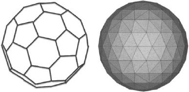
Figure 5.46. Geodesic spheres are made from polygons. The one on the left is made from hexagons and pentagons while the one on the right is made from triangles.

Figure 5.47. Geodesic dome array made from triangular planar arrays with 36 elements in a triangular lattice.

Figure 5.48. Active sector of the array depends upon the beam pointing direction.

An example of a geodesic dome array built from triangles is shown in Figure 5.47. Each triangular section is a panel containing 36 elements on a triangular grid. This array scans horizon to horizon by activating the appropriate subarrays to form an active aperture that points in the desired direction [15]. Each array element or subarray must have an RF on/off switch. When the subarray is active, then the switch is on and the element phase shifter is adjusted to form a coherent beam in the desired direction. Figure 5.48 demonstrates the concept of an active region that is a function of the beam pointing direction. The size of the active section depends upon α_max. For instance, the number of triangles in the active region may be 6 for a small α_max or the region enclosed by the dashed line in Figure 5.48 for a large α_max when the beam pointing direction is (θ_s1, _s1). Moving the beam to (θ_s2, _s2) moves the active region to the other side of the sphere (Figure 5.48). Beam scanning is accomplished by activating different sectors of the dome. A representative triangular section was built and tested. The subarray has 78 circular patch elements in a triangular grid (Figure 5.49). The antenna pattern was measured in the near field and compared well with the predicted pattern (Figure 5.50).

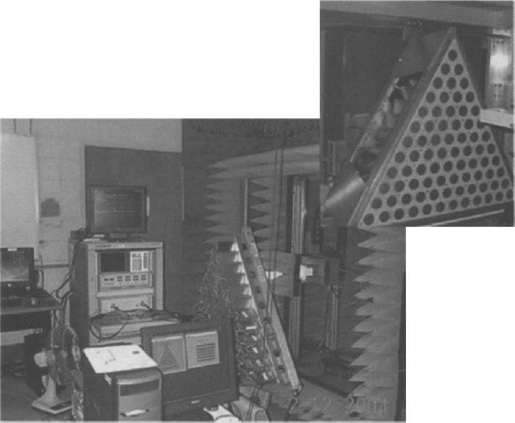
Figure 5.49. Subarray panel in a near-field test range. (Courtesy of Boris Tomasic, USAF AFRL [15].)

In order to make the manufacture and testing of the geodesic dome array as cheap as possible, all the polygons composing the surface should be of identical size. It turns out that there are only five types of regular polyhedron. Their characteristics are shown in Table 5.3. The more faces there are on a polyhedron, the more closely it approximates a sphere. As such, the icosahedron (composed of 20 equilateral triangles) seems the most likely candidate.

The 10-m-diameter Geodesic Dome Phased Array Antenna (GDPAA) Advanced Technology Demonstration (ATD) antenna shown in Figure 5.51 was built by Ball Aerospace & Technologies Corp. This array was developed to demonstrate multi-beam phased array capability for next generation Air Force Satellite Control Network stations [17]. Hexagonal and pentagonal panels in the geodesic dome contain many hexagonal subarrays. The hexagon subarrays have 37 elements (Figure 5.52) in a triangular grid. Only 36 of the elements are active, because the center element is devoted to calibration. The GDPAA tracks multiple satellites using multiple beams as shown in Figure 5.53. A very sophisticated beam management algorithm was developed to allow active section to overlap and cross while multiple beams simultaneously track multiple targets [15].

Figure 5.50. Measured and computed subarray patterns. (Courtesy of Boris Tomasic, USAF AFRL [15].)

5.4. DISTRIBUTED ARRAY BEAMFORMING

A distributed array collects signals from antennas at various locations and coherently combines them to form a beam. The signal combination occurs in real time or much later as is often done with radio telescopes. Data collected by each element is precisely time stamped at the element which has a precisely known location. The strict timing and location accuracy requires constant calibration, otherwise the phase errors would be too large to form a desirable coherent main beam. Distributed arrays are typically very sparse, so grating lobes are a problem that must be addressed through signal processing, element placement, and limited scanning.

Consider the fictional Very Long Baseline Interferometry (VLBI) array shown on the map of the United States in Figure 5.54. Such an antenna might be used in radio astronomy to form a huge aperture. The large distances between the reflector antenna elements make it impossible to use transmission lines to coherently combine signals to form a beam at the data collection site. Small element location errors produce major antenna pattern distortions described in Chapter 2. In order to determine the element signal phases, the data assembled by each element are tagged with the time from atomic clocks along with a GPS time stamp. The data are collected at a central location (shown by a star on the map). The timing of the data at each element is adjusted according to the atomic clock time stamp, and the estimated times of arrival of the signal at the elements. Each antenna is a different distance from the radio source, so an artificial time delay is added to the appropriate elements. If the position of the antennas is not known to sufficient accuracy or atmospheric effects are significant, fine adjustments to the delays in the signal processing must be made until a coherent beam is formed.

TABLE 5.3. Characteristics of Regular Polyhedron [16]

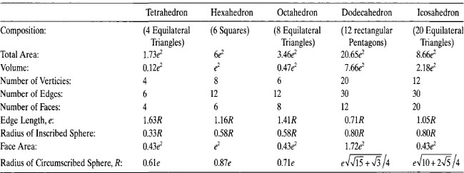
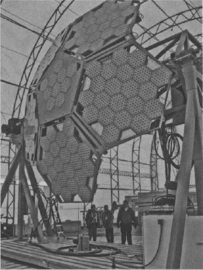
Figure 5.51. GDPAA ATD antenna. (Courtesy of Ball Aerospace & Technologies Corp.)

Figure 5.52. Hexagonal subarray for the GDPAA. (Courtesy of Ball Aerospace & Technologies Corp.)

Figure 5.53. Operational concept of the GDPAA. (Courtesy of USAF AFRL.)

Figure 5.54. Fictional VLBI array in the United States.

Figure 5.55. ALMA concept [(copyright © ALMA (ESO/NAOJ/NRAO)].

The VLA presented in Chapter 4 is one example of a VLBI array. Another example is the new VLBI array called the Atacama Large Millimeter/submillimeter Array, or ALMA [18]. It is an international collaboration between Europe, North America, and East Asia, with the Republic of Chile, to build and operate a radio telescope composed of 66 12-m and 7-m parabolic dishes in Chile’s Andes Mountains (Figure 5.55), at 5000 m above sea level. The telescope operates at frequencies from 31.25 GHz to 950 GHz. Array configurations from 250 m to 15 km will be possible. The ALMA antennas will be movable between flat concrete slabs built on the site. Figure 5.56 is a picture of one of the vehicles moving an antenna. Coherent beams can be formed in real time through the use of optical fiber feeds to a local data collection center.

5.5. TIME-VARYING ARRAYS

The properties of an array may quickly change with time through purposely time modulating array parameters or through the array element positions changing with time. In effect, the three-dimensional spatial problem becomes a four-dimensional space-time problem [19].

5.5.1. Synthetic Apertures

A synthetic aperture is a large aperture built over time by moving a smaller antenna and taking snapshots along the path. Radio telescopes frequently use the rotation of the earth to fill in an aperture. For instance, the radio telescopes at A1 and A2 in Figure 5.57 move to A1′ and A2′ then to A1″ and A2″ as the earth turns. Continually adding the snapshots together using proper phasing forms an image with much higher resolution than is only A1 and A2 were used alone.

Figure 5.56. Vehicle used to move an ALMA prototype element [(copyright © ALMA (ESO/NAOJ/NRAO)].

A synthetic aperture radar SAR is usually mounted on an airplane or satellite that passes over relatively immobile targets. The length of the antenna collection determines the resolution in the azimuth (along-track) direction of the image. If the antennas collect data over time, T, when the platform is moving at velocity, v, then the antenna is vT long, and the virtual beamwidth (resolution) of the antenna is approximately λ/vT. Figure 5.58 shows a cartoon of the space shuttle with a SAR. The footprint on the ground is one element pattern in the synthetic array. Pulses are transmitted as the radar moves relative to the ground. The returned echoes are Doppler-shifted (negatively as the radar approaches a target; positively as it moves away). Comparing the Doppler-shifted frequencies to a reference frequency allows many returned signals to be “focused” on a single point, effectively increasing the length of the virtual antenna [20].

Radar signals received by the SAR depend on the polarization and look angle of the antenna as well as the variations in shape and materials in the landscape [21]. SAR arrays frequently have dual polarized elements, so the array can transmit vertical and receive vertical or horizontal, or transmit horizontal and receive vertical or horizontal. Using these four polarization combinations produces different “views” of the terrain, because scattering is a function of polarization and look angle.

Figure 5.57. Synthetic aperture built using two radio telescopes at A1 and A2.

Figure 5.58. SAR imaging on the Space Shuttle.

Figure 5.59. SIR-B antenna before unfolding during deployment in space. (Courtesy of Ball Aerospace & Technologies Corp.)

SAR can detect changes (that might result from motion) in sequential images. When the pixels of two images of the same scene, but taken at different times, are aligned and then cross-correlated pixel by pixel, then the pixels that change between images are uncorrelated and easy to detect. Alterations in the landscape, such as subterranean tunneling, vehicle motion, glacier flow, earthquakes, and volcanic activity, produce uncorrelated pixels in the before and after images. The motion of a ground-based moving target such as a car is also detectable.

The Shuttle Imaging Radar B (SIR-B) experiment was launched on October 5, 1984, onboard the shuttle Challenger [22], SIR-B collected 15 million square kilometers of ocean and land surface data during a 16-hour period. The radar was mechanically tilted to obtain multiple radar images of a given target at different angles during successive shuttle orbits. The antenna array was put together in subarray panels that fold together for storage in the space shuttle as shown in Figure 5.59. Figure 5.60 shows the array unfolding to its full aperture size outside the space shuttle.

Figure 5.61 is a SAR image centered on Salt Lake City, Utah [22], This image was acquired by the Spaceborne Imaging Radar-C/X-Band Synthetic Aperture Radar (SIR-C/X-SAR) aboard the space shuttle Endeavour on April 10, 1994. The dark area is the Great Salt Lake. It is dark, because the surface is relatively smooth and the reflected signal obeys Snell’s law, so it bounces away from the radar. Vegetation, buildings, and mountains are rough surfaces and scatter in all directions. Consequently, the SAR receives signals from these areas and produce bright spots on the image for specular reflections.

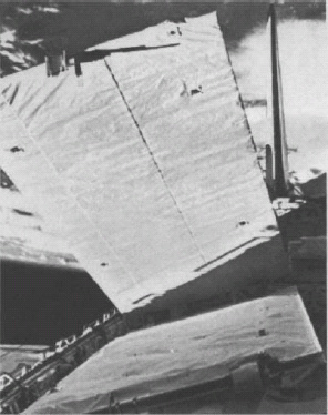
Figure 5.60. SIR-B antenna array unfolding for deployment on the space shuttle. (Courtesy of Ball Aerospace & Technologies Corp.)

The Spaceborne Imaging Radar-C/X-band Synthetic Aperture Radar (SIR- C/X-SAR) fit inside the Space Shuttle’s cargo bay as shown in Figure 5.62. Its mission was to make measurements of vegetation type, extent, and deforestation; soil moisture content; ocean dynamics, wave and surface wind speeds and directions; volcanism and tectonic activity; and soil erosion and desertification [22]. The SIR-C/X-SAR had antennas operating at 1.3GHz, 5.2GHz, and 10 GHz (Figure 5.63). The L-band and C-band phased arrays have both horizontal and vertical polarizations. The X-SAR array is a 12-m × 0.4-m X-band vertically polarized slotted waveguide array, which uses a mechanical tilt to change the beam-pointing direction between 15° and 60°. The beam electronically scans in the range direction ±23° from the nominal 40° off nadir position. Both SIR-C and X-SAR operate as either stand-alone radars or together. Roll and yaw maneuvers of the shuttle allow data to be acquired on either side of the shuttle nadir (ground) track. The width of the imaged swath on the ground varies from 15 to 90 km, depending on the orientation of the antenna beams and the operational mode.

Figure 5.61. SAR image of Salt Lake City, UT. (Courtesy of NASA JPL.)

5.5.2. Time-Modulated Arrays

In the time domain, the array factor for a linear array can be written as

Time-modulated arrays open and close switches in a prescribed sequence that causes the average array pattern to simulate a low sidelobe array amplitude taper. When the switch is on, the element connects to the feed network. If the switch is off, the element contributes no signal to the output. The switch on time, τ_n, determines the average element weights. Each switch rapidly turns on and off in synchronization to an external periodic signal having a period of T. An element whose switch is always on has a weight of 1, while an element whose switch is always off has a weight of 0. The amplitude weight on element n is the fraction of the period that a switch is on.

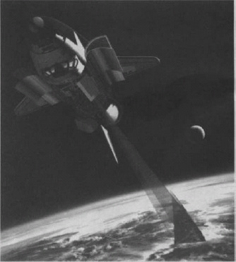
Figure 5.62. SIR-C concept. (Courtesy of Ball Aerospace & Technologies Corp.)

Figure 5.63. Photograph of the SIR-C antenna. (Courtesy of Ball Aerospace & Technologies Corp.)

The switches cannot control the phase of the signal.

The new time-varying weights result in the following time dependent array factor:

where

This equation implies that the array factor not only exists at the fundamental frequency, ω₀, but array factors also exist at all the harmonics of the switching frequency.

Time modulation was demonstrated using an X-band experimental corporate-fed array of eight collinear slots that had three diode switches [23], The center two elements were always on while each of the three switches controlled a pair of elements located symmetrically about the array center. Isolators on either end of the switch prevented impedance changes due to turning the switch on and off. The switching sequence begins with all the array elements turned on. A monotonically decreasing amplitude taper results when the outer pair (element numbers 1 and 8) turn off, then the next outer pair (element numbers 2 and 7) turn off, and finally the next (element numbers 3 and 6) turn off until only the center pair (4 and 5) remain on. The switches operated at a frequency of 10 kHz. The various on times were selected to give the correct low-sidelobe pattern after the signal was filtered.

The time-modulated low-sidelobe pattern gain is less than the gain of an equivalent static (no switching) amplitude tapered array due to the power lost through the additional array factors at the harmonics of the modulation frequency [24]. Expressions for the power loss are found in reference 24. A different array pattern exists at each harmonic. As an example, an array with a time-modulated 40-dB sidelobe taper has 3.53 dB less gain than a 40-dB sidelobe static amplitude tapered array. If the static array has an initial low-sidelobe amplitude taper, then the time modulation will be more efficient. For instance, if an array with a static 30-dB amplitude taper is lowered to 40 dB through time modulation, then it has a gain that is 0.51 dB less than that of a 40-dB sidelobe static amplitude tapered array.

5.5.3. Time-Varying Array Element Positions

Some Communications and sensing applications need high-gain arrays in space. Element positions in these arrays vary when the surface of the array flexes or individual elements on independent platforms change position. The support structure for a large array on the ground is made with steel and concrete. In space, however, the lightweight materials used in construction cannot provide the same solid support. Even though strong structural supports can be made viable for space, vibrations induced by antenna deployment, temperature differences, orbit changes, and so on, cause the array aperture to undulate. Small vibrations at high antenna frequencies are disastrous for the main-beam gain. Element displacements add unwanted phase to the signals received at each element. Without proper compensation, these signals do not add coherently to form a main beam, resulting in antenna performance degradation.

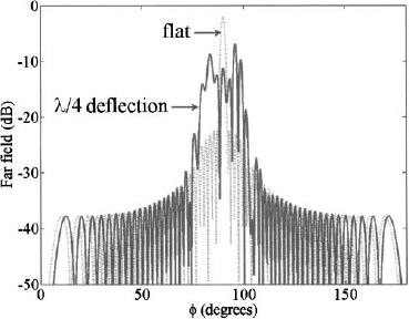
Example. A low-sidelobe 50-element linear array with element spacing of 0.5λ has a sinusoidal deflection with an amplitude of λ/2 as shown in Figure 5.64. Plot the array factors.

If the array is not phase compensated, then the main beam is severely distorted as shown in Figure 5.65. Phase compensation restores the array factor to near perfection if the element locations are known.

Elements of an array that are on different moving platforms are another type of time-varying aperture. For instance, antenna elements may be on individual unmanned aerial vehicles flying in formation. Beamforming consists of a wireless network that collects and coherently adds the signals from all the elements.

The Techsat 21 space-based radar [25] is a proposed cluster of micro-satellites that cooperate to form one large virtual satellite (Figure 5.66). Each satellite has roughly a 4-m² phased array, operating at 10 GHz. There are 4 to 20 satellites per cluster with cluster diameters of 100-1000 m. Orbits vary from 700 to 1000 km above earth. Satellites in the cluster communicate with each other and share the processing, Communications, and mission functions. The benefits of this approach include [26]:

1. The ability to create extremely large apertures.
2. Increased system reliability, because the failure of a single satellite does not result in complete system failure.

   

   Figure 5.64. Small λ/2 deflection in a linear array of 50 point sources.

   

   Figure 5.65. The array factor due a to λ/2 deflection compared to an array factor with no deflection.

   

   Figure 5.66. Proposed Techsat 21 configuration in orbit.

3. Easier upgrades to the satellites, since the satellites can be replaced one at a time instead of all at once.
4. Low costs due to satellite mass production and small launch payloads.
5. Improved survivability to natural and man-made threats due to the separation between satellites.
6. The ability to reconfigure and optimize the satellite formation for a given mission, enhanced survivability, and increased reliability.

Each satellite transmits a different frequency or other orthogonal signal, but receives all the signals from the other satellites in the formation. Although the absolute position of a satellite must be accurately known, the relative positions between satellites have the stringent requirement of a fraction of a wavelength in order to coherently sum the signals to form a beam. As shown in Chapter 2, the random element position errors determine the gain of the array.

GPS provides absolute timing to 100 ns. Differential GPS can provide relative position knowledge of 10 cm and timing to 20 ns, and an ultra stable oscillator provides local time precision of 5 ps over the maximum signal integration time of 5 s. Intersatellite Communications regularly update position and timing measurements. The actual satellite position with respect to other satellites in the array is measured using laser ranging, to provide relative positions with an error significantly less than a wavelength at the X-band. Thus, positional errors of the satellites are modeled as deviations from the nominal positions, having (a) a random but known component on the order of meter and (b) a random but unknown component on the order of 3 mm. Phase compensation corrects the known errors and the unknown errors raise the sidelobe level and lower the gain.

Example. An array with 64 elements that are randomly distributed in a 3.5λ × 3.5λ × 3.5λ volume. Plot the incoherent array factor and the array factor with a coherent beam steered to (θ_s, _s) = (45°, 0°).

The randomly distributed volume array is shown in Figure 5.67. The uniformly weighted array factor appears in Figure 5.68. It consists of many very small lobes of about the same height. If the elements are phased to form a coherent beam at (θ, ) = (45°, 0°), then the array factor in Figure 5.69 results with a desired main beam.

The High-Frequency Surface Wave Radar (HFSWR) is deployed along a coast to detect boats far from shore [27]. Finding an area along the water to build a long array is often difficult, so it has been proposed to place the array elements on buoys that are tied to the sea bottom. Ocean waves cause movement of the elements that are a function of the length of the cable and the sea state or height of the waves. A computer model of the ocean calculated the element locations as a function of x, y, and z [28]. As long as the location of the element is known, then appropriate phase corrections can be applied to compensate the pattern.

As an example, consider the case of a 10-element linear array with a desire spacing of λ/2 on top of an ocean with 0.9- to 1.5-m waves (sea state 3). The array configuration changes with time as shown by the time varying azimuth antenna pattern in Figure 5.70. The sidelobes increase from -13 dB to as much as −6.6 dB at t = 10s. These waves do not cause a change in the beam-pointing direction. Phase corrections result in the pattern shown in Figure 5.71. The array pattern is restored except in the far-out sidelobe region. This concept will be demonstrated by building a small array of monopoles located on as shown in Figure 5.72. One zodiac with the HF radar equipment and monopole antennas are tethered to shore during testing. Additional zodiacs with monopoles will be added in the future.

Figure 5.67. Random array of 64 point sources in a 3.5λ × 3.5× × 3.5λ volume.

Figure 5.68. Incoherent array factor for the random array.

Figure 5.69. Array factor with a coherent beam pointing at (θ, ) = (45°, 0°).

Figure 5.70. Uncorrected antenna pattern as a function of time. (Courtesy of Régis Guinvarc’h, SONDRA, Supelec.)

Figure 5.71. Corrected antenna pattern as a function of time. (Courtesy of Régis Guinvarc’h, SONDRA, Supelec.)

Figure 5.72. Picture of the monopole located on a zodiac. The elements were on the ocean and tethered to the land by ropes. (Courtesy of Régis Guinvarc’h, SONDRA, Supelec.)

Platform vibrations also result in time-varying elements in an array. The element positions can be estimated by mounting some near field reference sources on rigid frames that do not vibrate. The beamformer uses the estimated position information to correct the distorted pattern of the antenna array. A 5.8-GHz 8-element array with artificially displaced element positions was built to emulate the vibration effect [29]. The proposed calibration approach estimated the position with deviations under 4% of the free space wavelength.

REFERENCES

1. L. Josefsson and P. Persson, Conformal array synthesis including mutual coupling, Electron. Lett., Vol. 35, No. 8, 1999, pp. 625–627.
2. M. T. Borkowski, Solid state transmitters, in Radar Handbook, M. Skolnik, ed., New York: McGraw-Hill, 2008, pp. 11.1–11.36.
3. R. Hendrix, Aerospace system improvements enabled by modern phased array radar—2008, IEEE Radar Conference, 2008, 26-30 May 2008, pp. 1–6.
4. O. M. Bucci, G. D’ Elia, and G. Romito, Power synthesis of conformal arrays by a generalised projection method, IEE Proc., Microwaves, Antennas Propagat., Vol. 142, No. 6, 1995, pp. 467–471.
5. J. A. Ferreira and F. Ares, Pattern synthesis of conformal arrays by the simulated annealing technique, Electron. Lett., Vol. 33, No. 14, 1997, pp. 1187–1189.
6. E. Botha and D. A. McNamara, Conformal array synthesis using alternating projections, with maximal likelihood estimation used in one of the projection operators, Electron. Lett., Vol. 29, No. 20, 1993, pp. 1733–1734.
7. O. M. Bucci and G. D’Elia, Power synthesis of reconfigurable conformal arrays with phase-only control, IEE Proc. Microwaves Antennas Propagat., Vol. 145, No. 1, 1998, pp. 131–136.
8. M. R. Frater and M. J. Ryan, Electronic Warfare for the Digitized Battlefield, Boston: Artech House, 2001.
9. M. R. Morris. Wullenweber antenna arrays, May 28, 2009, http://www.navycthistory.com/WullenweberArticle.txt.
10. F. Adcock, Improvement in Means for Determining the Direction of a Distant Source of Electromagnetic Radiation, 1304901919, B.P. Office, 1917.
11. E. J. Baghdady, New developments in direction-of-arrival measurement based on Adcock antenna clusters, Aerospace and Electronics Conference, 1989, pp. 1873–1879.
12. F. Chauvet, Conformal, wideband, dual polarization phased antenna array for UHF radar carried by airship, The University Pierre et Marie Curie Paris 6, 2008.
13. B. Tomasic, J. Turtle, and L. Shiang, Spherical arrays—Design considerations, 18th International Conference on Applied Electromagnetics and Communications, 2005, pp. 1–8.
14. B. Tomasic, J. Turtle, and S. Liu, The Geodesic Sphere Phased Array Antenna for Satellite Communication and Air/Space Surveillance—Part I, AFRL-SN-HSTR-2004-031, January 2004.
15. L. Shiang, B. Tomasic, and J. Turtle, The geodesic dome phased array antenna for satellite operations support—Antenna resource management, Antennas and Propagation Society International Symposium, June 2007, pp. 3161–3164.
16. Chemical Rubber Company, CRC Standard Mathematical Tables and Formulae, Boca Raton, FL: CRC Press, 1991, p. v.
17. B. Tomasic, J. Turtle, L. Shiang et al., The geodesic dome phased array antenna for satellite control and communication—Subarray design, development and demonstration, IEEE International Symposium on Phased Array Systems and Technology, 2003, pp. 411–416.
18. About ALMA Technology, May 27, 2009, http://www.almaobservatory.org/.
19. H. E. Shanks and R. W. Bickmore, Four-dimensional electromagnetic radiators, Can. J. Phys., Vol. 37, 1957, pp. 263–275.
20. G. W. Stimson, Introduction to Airborne Radar, El Segundo, CA: Hughes Aircraft Co., 1983.
21. R. K. Raney, Space-based remote sensing radars, in Radar Handbook, M. Skolnik, ed., New York: McGraw-Hill, pp. 18.1–18.70, 2008.
22. Imaging Radar @ Southport, May 28, 2009; http://southport.jpl.nasa.gov/.
23. W. Kummer, A. Villeneuve, T. Fong et al., Ultra-low sidelobes from time- modulated arrays, IEEE Trans. Antennas Propagat., Vol. 11, No. 6, 1963, pp. 633–639.
24. J. C. Bregains, J. Fondevila-Gomez, G. Franceschetti et al., Signal radiation and power losses of time-modulated arrays, IEEE Trans. Antennas Propagat., Vol. 56, No. 6, 2008, pp. 1799–1804.
25. H. Steyskal, J. K. Schindler, P. Franchi et al., Pattern synthesis for TechSat21—A distributed space-based radar system, IEEE, Antennas Propagat. Mag., Vol. 45, No. 4, 2003, pp. 19–25.
26. R. Burns, C.A. McLaughlin, J. Leitner, and M. Martin, “TechSat 21: formation design, control, and simulation,” IEEE Aerospace Conference Proceedings, 2000, pp. 19–25
27. L. Sevgi, A. Ponsford, and H. C. Chan, An integrated maritime surveillance system based on high-frequency surface-wave radars. 1. Theoretical background and numerical simulations, IEEE, Antennas Propagat. Mag., Vol. 43, No. 4, 2001, pp. 28–43.
28. A. Bourges, R. Guinvarc’h, B. Uguen et al., A simple pattern correction approach for high frequency surface wave radar on buoys, First European Conference on Antennas and Propagation, 6–10 Nov. 2006, pp. 1–4.
29. W. Qing, H. Rideout, Z. Fei et al., Millimeter-wave frequency tripling based on four-wave mixing in a semiconductor optical amplifier, Photonics Technol. Lett., IEEE, Vol. 18, No. 23, 2006, pp. 2460–2462.