
Shading is the Maya term for applying colors and textures, known in Maya as shaders. A shader defines an object's look—its color, tactile texture, transparency, luminescence, glow, and so forth.
Topics discussed in this chapter include:
Shader Types
Shader Attributes
Texturing the Axe
Textures and Surfaces
Texturing the Red Wagon
Working with and Creating UVs
After you model your objects, Maya assigns a default shader to them with a neutral gray color. This is to allow them to render and display properly. If no shader is attached to a surface, an object cannot be seen.
Shading is the proper term for applying a renderable color, surface bumps, transparency, reflection, shine, or similar attributes to an object in Maya. It is closely related to, but distinct from, texturing, which is what you do when you apply a map or other node to an attribute of a shader to create some sort of surface detail. For example, adding a scanned photo of a brick wall to the Color attribute of a shader that you assign to a model in Maya is considered applying texture. Adding another scanned photo of the bumps and contours of the same brick wall to the Bump Mapping attribute is also considered applying a texture. Nevertheless, because textures are often applied to shaders, the entire process of shading is sometimes informally referred to as texturing. Applying textures to shaders is also called texture mapping or simply mapping. You map a texture to the color node of a shader that is assigned or applied to a Maya object.
Shaders are based on nodes. Each node holds the attributes that define the shader. With shaders, akin to the hierarchies and groups of models, you create Shader networks of interconnected nodes. These networks can be simple or they can be intricate and involved, as when several render nodes are used to create complex shading effects.
Each shader, also known as a shading group, comprises a set of material nodes. Material nodes are the Maya nodes that hold all the pertinent rendering information about the object to which they are assigned, such as their color, opacity, or shininess. The shading groups are the nodes that allow the connection between the surface and the material you've created. When you edit the shader through the Attribute Editor, as you will do later in this chapter, you edit its material node.
There are two ways to create and edit shaders in Maya. As you learn about shading in this chapter, you will deal primarily with the Hypershade window as opposed to the Multilister. See Chapter 2, "Jumping in Headfirst, with Both Feet," and Chapter 3, "The Maya 2009 Interface," for the layout of these windows and for a hands-on introduction to the Hypershade. You can access either window by choosing Window → Rendering Editors. Shading in Maya is almost always done hand in hand with lighting. At the very least, textures are tweaked and edited in the lighting stage of production. Because the appearance of an object depends on light, in this chapter's exercise you'll create some lights as you create textures. You'll learn more about lighting in Chapter 10, "Maya Lighting."
Open the Hypershade by choosing Window → Rendering Editors → Hypershade. In the left column of the Hypershade window, you will see a listing of Maya shading nodes (Figure 7.1). The first section displays Surface nodes, aka material nodes or shader types. Of these shader types, you'll find five that are common to other animation packages as well. You'll use two of these later in this chapter.

To understand a bit more about shaders, consider what makes objects appear as they do in the real world. The short answer is light. The way light bounces off an object defines how you see that object. The surface of the object may have pigments that affect the wavelength of light once it reflects off it, giving the surface color. Other features of that object's surface also dictate how light is reflected.

For the most part, shader types address the differences in how light bounces off surfaces. Most light, once it hits a surface, diffuses across an area of that surface. It may also reflect a hot spot called a specular highlight. The shaders in Maya differ in how they deal with specular and diffuse parameters according to the specific math that drives them. As you learn about the shader types, think of the things around you and what shader type would best fit them. Some Maya shaders are specific to creating special effects, such as the Hair Tube shader or the Use Background shader. It is important to learn the fundamentals first, so we will cover the shading types you will be using right off the bat.
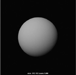
The most common shader type is Lambert, an evenly-diffused shading type found in dull or matte surfaces. A sheet of paper, for example, is a Lambert surface.
A Lambert surface diffuses and scatters light evenly across its surface, in all directions. (See Figure 7.2.)

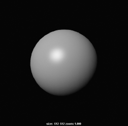
Phong shading, named after its developer, Bui Tuong-Phong who created it in 1975, brings to a surface's rendering the notions of specular highlight and reflectivity. A Phong surface reflects light with a sharp hot spot, creating a specular highlight that drops off sharply. (See Figure 7.3.) You'll find that glossy objects such as plastics, glass, and most metals take well to Phong shading.
Also named after its developer, James Blinn, the Blinn shading method brings to the surface a highly accurate specular lighting model that offers superior control over the specular's appearance. (See Figure 7.4.) A Blinn surface reflects light with a hot spot, creating a specular that diffuses somewhat more gradually than a Phong. This creates a shader that is good for use on shiny surfaces and metallic surfaces.
The Phong E shader type expands the Phong shading model to include more control over the specular highlight. A Phong E surface reflects light much as a regular Phong does, but it has more detailed control over the specular settings to adjust the glossiness of the surface. (See Figure 7.5.) This creates a surface with a specular that drops off more gradually and yet remains sharper than a Blinn. Phong E also has greater color control over the specular than do Phong and Blinn, giving you some more options for metallic reflections.
The Anisotropic shader is good to use on surfaces that are deformed, such as a foil wrapper or warped plastic. (See Figure 7.6.)

Anisotropic refers to something whose properties differ according to direction. An Anisotropic surface reflects light unevenly and creates an irregular-shaped specular highlight that is good for representing surfaces with directional grooves, like CDs. This creates a specular highlight that is uneven across the surface, changing according to the direction you specify on the surface. By contrast with Blinn and Phong types, the specular highlight is evenly distributed to make a circular highlight on the surface.
A Layered shader allows the stacking of shaders to create complex shading effects, which is useful for creating objects composed of multiple materials. (See Figure 7.7.) By using the Layered shader to texture different materials on different parts of the object, you can avoid using excess geometry.

You control Layered shaders by using transparency maps to define which areas show which layers of the shader. You drag material nodes into the top area of the Attribute Editor and stack them from left to right, the left being the topmost layer assigned to the surface.
Layered shaders are valuable resources to control compound and complex shaders. They are perfect for putting labels on objects or adding dirt to aged surfaces. You will use a Layered shader in the Axe Texturing exercise later in this chapter.
A Ramp texture is a gradient that can be attached to almost any attribute of a shader as a texture node. Ramps can create smooth transitions between colors and can even be used to control particles. (See Chapter 12, "Maya Dynamics and Effects," for how a ramp is used to control particles.) When used as a texture, a ramp can be connected to any attribute of a shader to create graduating color scales, transparency effects, increasing glow effects, and so on. You will use Ramp textures later in this chapter.
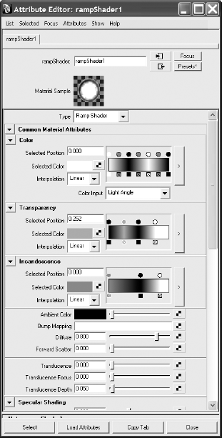
The Ramp shader is a self-contained shader node that automatically has several Ramp texture nodes attached to its attributes. These ramps are attached within the shader itself, so there is no need to connect external Ramp texture nodes. This makes for a simplified editing environment for the shader because all the colors and handles are accessible through the Ramp shader's own Attribute Editor, as shown in Figure 7.8.
To create a new color in any one of the horizontal ramps, click in the swatch to create a new ramp position. Edit its color through its Selected Color swatch. You can move the position by grabbing the circle right above the ramp and dragging left or right. To delete a color, click the box beneath it.
Ramp textures are automatically attached to the Color, Transparency, Incandescence, Specular Color, Reflectivity, and Environment attributes of a Ramp shader. In addition, a special curve ramp is attached to the Specular Roll Off to allow for more precise control over how the specular highlight diminishes over the surface.
Shaders are composed of nodes just as other Maya objects. Within these nodes, attributes define what shaders do. Here is a brief rundown of the common shader attributes with which you'll be working.
- Color
An RGB or HSV value that defines what color the shader is when it receives a neutral color light. For more on RGB and HSV, see Chapter 1, "Introduction to Computer Graphics and 3D."
- Transparency
The higher the Transparency value, the less opaque and more "see-through" the object becomes.
Although usually expressed in a black-to-white gradient, with black being opaque or solid and white being totally clear, transparency can have color. In a color transparency, the shader's color shifts because only some of its RGB values are now transparent as opposed to the whole.
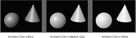
- Ambient Color
This color affects the Color attribute of the shader as more ambient light is created in the scene. Ambient color tends to flatten an object because this attribute evenly colors the object. This attribute is primarily used to create flat areas and should be used with care. The default is black, which keeps the darker areas of a surface dark. The lighter the ambient color, the lighter those areas will be. A bright Ambient Color setting will flatten out an object, as shown in Figure 7.9
- Incandescence
This is the ability to self-illuminate. Objects that seem to give off or have their own light, such as an office's fluorescent light fixture, can be given an incandescence value. Incandescence will not, however, light objects around it in regular renders, nor will it create a glow. It will also serve to flatten the object into a pure color. As you will see in Chapter 11, incandescence can also help light a scene in mental ray's Final Gather rendering. The value of incandescence (as well as the color) of an object is used to calculate the overall brightness in a Final Gather scene. (See Figure 7.10.)
- Bump Mapping
This attribute creates a textured feel to the surface by adding highlights and shadows to the render. It will not actually alter the surface of the geometry, although it will make the surface appear to have ridges, marks, scratches, and so forth. The bump map has to be a texture node such as a ramp, a fractal noise, or an image file. The more intense the variation in tones of that map, the greater the bump. Bump maps are frequently used to make surfaces look more real, as nothing in reality has a perfectly smooth surface. Using bumps very close up may create problems, so bumps are generally good for adding inexpensive detail to a model that is not in extreme close-up. (See Figure 7.11.)
Note
Close-up geometry, where you have to change the topology of the model physically using texture maps, will require displacement maps. We will cover displacement maps later in this chapter.
- Diffuse
This value governs how much light is reflected from the surface in all directions. When light strikes a surface, light disperses across the surface and helps to illuminate it. The higher this value, the brighter its object is when lit because more of the striking light is reflected from the surface. The lower the diffuse value is, the more light will be "absorbed" into the surface, yielding a darker result, especially in areas that are not well lit. Metals have very low diffuse values because they rely on reflections and direct light. (See Figure 7.12.)
- Translucence and Translucence Focus
The Translucence and Translucence Focus attributes give the material the ability to transmit light through its surface, like a piece of canvas in front of a light. At a value of 1 for Translucence, all light shines through the object; at 0, none does. The Translucence Focus attribute specifies how much of that light is scattered. A light material such as paper should have a high translucence focus, and thicker surfaces should have low focus rates.
- Glow Intensity
Found in the Special Effects section of the Attribute Editor, the Glow Intensity attribute adds a glow to the object, as if it were emitting light into a foggy area. (See Figure 7.13.) We will add glow to an object in Chapter 10.
- Matte Opacity
Objects rendered through Maya generate a solid matte. Where there is an object, the matte is white; where there is nothing, the matte is black. This helps compositing programs, which bring together elements created independently into a single composite scene, to separate rendered CG from their backgrounds. Turning the slider down decreases the brightness of the object's matte, making it appear more transparent. This is usually used for compositing tricks or to make an object render in RGB but not appear in any composites. For more information about mattes, see both the sidebar "Image Mattes" in this chapter and Chapter 11, "Maya Rendering."
- Raytrace Options
With raytracing, you can achieve true reflections and refractions in your scene. This subset of attributes allows you to set the raytracing abilities of the shader. See Chapter 11 for more on raytracing.
Some attributes are available only with certain shader types. The following are the attributes you'll see for the Phong, Phong E, and Blinn shaders.
- Specular Color
The color of the highlights on a shiny surface. Black produces no specular, and white creates a bright one.
- Reflectivity
The amount of reflection that is visible in the surface. The higher the value, the more reflective the object will render. Increasing this value increases the visibility of the Reflected Color attribute or of true reflections in the scene when raytraced.
- Reflected Color
Gives the surface a reflection. Texture maps are generally assigned to this attribute to give the object a reflection of whatever is in the image file or texture without having to generate time-consuming true reflections with a raytraced render. Using raytracing to get true reflections, however, is the only way to generate reflections of other objects in the scene.
- Cosine Power
Only available with a Phong shader. This attribute changes the size of the shiny highlights (aka specular) on the surface. The higher the number; the smaller the highlight will look.
- Roughness, Highlight Size, Whiteness
Control the specular highlight on a Phong E surface only. They control specular focus, amount of specular, and highlight color, respectively.
- mental ray attributes
Because Autodesk now integrates features of its mental ray rendering engine into Maya, there is usually a set of mental ray options in the Attributes of an object. Shaders are no different. If you open the mental ray heading in the Attribute Editor for a shader, you'll notice a few attributes, such as Reflection Blur and Irradiance, as well as a few ways to override Maya's shading attributes with mental ray's own.
An in-depth discussion of the mental ray attributes is beyond the scope of this introductory text, but it is a good idea to know this brief section is here and available to you once you have more experience with rendering and you want to work with mental ray at its more advanced levels in Maya. We will work with mental ray in Chapters 10 and 11.


In this section, you will add shaders to a NURBS modeled axe to make it look real; and in the next chapter, you'll import this axe into an animation exercise. Starting animation on a project and then replacing it with a finished and textured model is actually a fairly common practice with Maya.
Load axe_texture_A.mb from the Axe project on the CD.
You'll start by texturing the metal parts of the axe. Even though you can find a good metal to use for your axe head in Maya's shader library or on Autodesk's website, for this exercise you will make a simple metal from scratch. Because the look of real metals is greatly affected by their surroundings (that is, by the reflections of the environment), metal is one of the toughest materials to create and light. In many cases, metals are lighted and rendered with HDR Image Based Lighting, a technique too advanced for this book. It will be easier to learn once you are more familiar with lighting and rendering with Maya.
Note
Autodesk's website lists several pre-made shaders for your use. Maya also includes a shader library on its installation CD.
First, set up your render parameters so that you can render out your axe while you are tweaking the Metal shader to get it right.
Choose Window → Rendering Editors → Render Settings, or click Insert: (

In the Image Size section under the Common tab, set Presets to 640 × 480. In the Anti-aliasing Quality section under the Maya Software tab, use the Intermediate Quality preset. This will give you a good look for the final render with a short render time.
Open the Hypershade window, and click Phong in the Create Maya Nodes section. A new Phong shader will show up in both the top and the bottom parts of the Hypershade window.
Double-click the phong1 shader node in the Hypershade window to open the Attribute Editor and name the shader Metal.
Click the gray swatch next to the Color attribute to open the Color Chooser. Select a light blue-gray. In the Slider section, the HSV values should be something like H: 207, S: 0.085, and V: 0.80. Click Accept.
Back in the Attribute Editor for the shader, click the gray swatch for the Specular Color. By changing this color, you control the hue and brightness of the highlights on this surface. Use a bright faded blue with HSV values of H: 208, S: 0.20, and V: 0.90.
Increase the spread of the specular highlights by changing the Cosine Power from the default of 20 to 2.0. This creates a large area for the bright highlights, implying a polished reflective surface.
To assign the shader to the surfaces, select both sides of the axe head. In the Hypershade, right-click the shader node (in either the upper or lower window), and choose Assign Material to Selection from the shortcut menu. Figure 7.14 shows the shader.
Make sure your perspective view is active, and click the Render the Current Frame button (

This creates a simple Metal shader that will work well overall. To create a more polished look for the axe head, you can add a reflection to it using an Environment texture node. This node creates a 3D texture node in the scene that will project its contents onto the Material attribute to which it has been connected. As an object animates through the scene, different parts of the texture will be reflected on its surface.
In the Metal shader's Attribute Editor, click the Map button next to the Reflected Color attribute, as shown in Figure 7.15. This attaches a new node to create a reflection and opens the Create Render Node window. Click the Environment Textures section and select Env Chrome. An environment texture will provide an interesting reflection.
Move the Reflectivity slider from 0.50 to 0.85. The higher this number, the more prominent the Reflected Color will reflect in the surface. Figure 7.16 shows the axe before and after a reflection. The Env Chrome reflection texture makes the axe look polished by reflecting a grid representing the ground and a bright blue sky.


After you create the Env Chrome texture, you'll see a green object in the Modeling windows at the origin, as shown in Figure 7.17. This is the Env Chrome's placement node. You can manipulate this node just as you manipulate other Maya objects—in other words, move, rotate, and scale it.
Altering this will change how the environment chrome projects itself in the scene. For example, if you increase the size of this placement node, the grid showing in the reflection of the axe will get larger. For more on projections and placement nodes, see the "Texture Nodes" section later in this chapter.
A glossy cherrywood would look good for the handle, so a Phong shader would be best.
In the Hypershade, choose Create → Materials → Phong. Set Diffuse to 0.70, Specular Color to a light gray, and Cosine Power to 50.
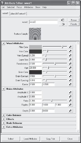
Click the Map button for the color. In the Create Render Node window, select Wood in the 3D Textures section. Figure 7.18 shows this texture in the Attribute Editor.
In the Wood's Attribute Editor, adjust Filler Color to a nice reddish brown with an HSV of 8.5, 0.85, and 0.43. Change Vein Color to a darker version of the filler with HSV color values of 8.5, 0.75, and 0.08, respectively.
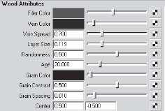
Change Vein Spread to 0.70, change Layer Size to 0.119, and darken Grain Color a bit by pulling the slider to the left, but not all the way, as shown in Figure 7.19. This will give you a nice dark cherrywood.
The Wood texture is a projected 3D texture; it's projected from a source onto the object using a placement node, just like the Env Chrome on the axe head's reflection. To assign the Wood texture from the Hypershade, select the handle and right-click the shader to select Assign Material to Selection, or MMB+click and drag the icon onto the handle in the viewport. For more on projected textures, see the "Texture Nodes" section later in this chapter.
Note
You can assign a shader to any object by MMB+clicking and dragging its icon from the Multilister or Hypershade to the object in the viewport.
To see this dark texture on your object, create a new light in the scene. In the main menu, choose Create → Lights → Ambient Light. (For more on lights, see Chapter 10.) Open the Attribute Editor for the light by pressing Ctrl+A or by double-clicking its icon on the Lights tab in the Hypershade. Increase the Intensity attribute to 2.5.
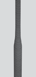
Render a frame of the axe handle up close, as shown in Figure 7.20. Notice how the wood repeats on the handle and creates an undesirable texture. Adjust the wood's texture placement.
To get to the Wood texture's placement node, open the Hypershade. Drag the Wood shader to the Hypershade work area (bottom half). Right-click the wood and choose Graph Network from the shortcut menu. You could also select it and click the Input Connections button (

Double-click the place3dTexture node to open its Attribute Editor.
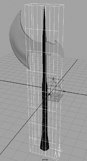
Click the Fit to Group BBox button to position the placement node for the wood around the handle automatically. In your viewport, you'll see the green placement node around the handle, as shown in Figure 7.22.
Rendering a frame reveals that the wood still does not look quite right. Select the placement node in the viewport, and rotate it in Z to 90. Click the Fit to Group BBox button again to rescale it to fit the handle. This will not rotate it back to the way it was; it will only scale it to fit the extent of the object to which it's assigned.
Render another frame, and you'll see the wood veins running the length of the handle. It looks more like wood now, but it still repeats too much.
Instead of moving and scaling the texture placement node and rendering multiple times to get the wood placement just right, you can use Maya's Interactive Photorealistic Rendering (IPR) to see your changes in real time. Click the IPR Render the Current Frame button (

The Render View window shows a lower-quality render of the axe. It will prompt you to select a region to begin tuning. Drag a marquee selection in the Render View window around the handle. IPR refreshes that part of the window. Every change you make to the texture placement node prompts IPR to update that section of the render, giving a fast update on the positioning and scale of the Wood texture.
Select the texture placement node and scale it up in the three axes until you get a good-looking grain. Figure 7.23 shows a well-spaced wood grain.

The scene file
axe_texture_B.mbin the Axe project on the CD will bring you up to this point.

Currently, the entire length of the handle is shaded as wood, including the top spike. The spike on the axe head should be metal like the axe head.
You can approach this in two ways: with geometry or with shaders. If you manipulate geometry, you select a horizontal isoparm and detach the spike portion of the handle to make it a separate surface. You then assign a Metal shader to the new tip surface.
Using a shader instead of cutting up or creating more geometry can be desirable in many instances. For example, you may not be able to detach surfaces like this all the time.
The Layered shader is a normal surface shader that allows you to stack materials on top of each other to assign to a surface. You control which layer of material is exposed and by how much by assigning transparency values or textures to each layer. Use a Ramp texture to specify where on the handle the wood stops and the metal starts.
To create a Layered shader, follow these steps:
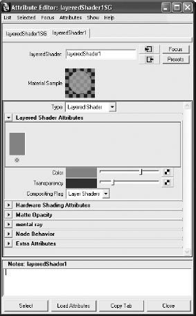
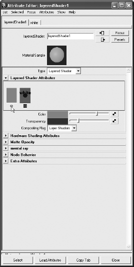
Select the axe handle, and in the Rendering menu set, choose Lighting/Shading → Assign New Material → Layered Shader to open the Attribute Editor, as shown in Figure 7.24. By default, the Layered shader contains a green layer in the top of the Attribute Editor window. From left to right, the layers are displayed in the order in which they appear from top to bottom as they are assigned to the surface. (This means that the leftmost shader in the Layered shader is on top of all the others.)
Using the Hypershade, MMB+click and drag the metal material you've made into the top region of the Layered shader's Attribute Editor window. To delete the default green material, click the X'ed square beneath it. The Material Sample icon in the Attribute Editor turns into the metal.
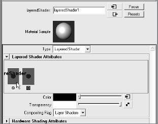
MMB+click and drag the wood material into the Layered shader's Attribute Editor. Make sure it is placed to the left of the metal material. If the materials are already in place, you can rearrange their order by MMB+clicking and dragging them left or right of the other materials in the Attribute Editor. Notice in Figure 7.25 that the Material Sample icon changed to the wood material. The wood is now the top layer, so only it will show until you give it some transparency to reveal some metal at the tip.
Note
You can see the names of the materials in the Layered shader by pointing to the icons.
Click the Wood Shader icon in the Layered shader's Attribute Editor to highlight it. Notice that the Transparency Map button (as well as Color) is now a square with an arrow (

When an attribute is already mapped, its Map button turns from a checkerboard to an Input Connection icon. Clicking it opens the Attribute Editor for whatever node is attached to that attribute. In this case, clicking the Map button opens its Attribute Editor because the wood material was assigned to this layer. Here you need to attach a transparency ramp to control where the metal tip starts and the wooden handle ends.
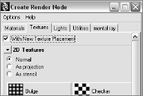
Click the Map button for the wood's Transparency attribute. Create a Ramp texture node. Make sure the Normal radio button is checked and not the As Projection or As Stencil radio button.
In the ramp's Attribute Editor, change Interpolation to None, and change Type to U Ramp.
Delete the middle (green) color by clicking the square to the right of green's position. Select the bottom (red) color by clicking its round handle on the left of the ramp. Change the Selected Color attribute to white. Drag it all the way to the bottom of the ramp.
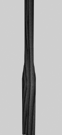
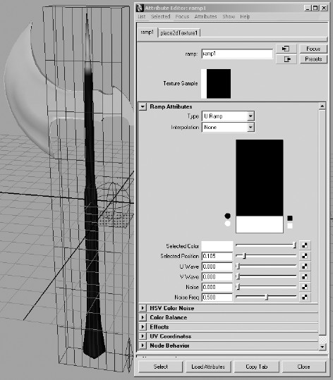
Select the top color (blue) and change it to black. Drag the handle down the ramp to a Selected Position of 0.105. Figure 7.26 shows the ramp position and the axe. If you're in Texture Display mode in the perspective view (press the 6 key), you'll see that the tip of the model is a blue-gray color (the metal) and the bottom of the handle is a reddish brown (the wood). As you adjust the position of the white color on the ramp, notice how the spike and handle change.
In the Hypershade, choose Edit → Delete Unused Nodes to purge all unused shading nodes from your scene. Make sure your Layered shader and Metal shader are assigned, of course.
Render out a frame of the axe. Save this frame in the render buffer by clicking Keep Image (

Select the axe's top node and rotate it about 45 degrees in Z to angle it. Render a frame at this point. Notice how the grain of the wood has changed. Use the scroll bar to toggle back and forth and compare these two images, as shown in Figure 7.27.
When a projected texture, such as the wood, does not "stick" to an object and the object seems to move through the texture, the object is said to be "swimming" through the projection. The wood is being projected by the 3D placement node that you positioned to get the grain just right, so you'll need to group the texture node under the axe's top node. When the axe moves, the texture will stick with it, maintaining its orientation with the axe.
Rotate the axe back to 0 in Z. Select the place3dTexture2 node from either the viewport (it's the green texture you scaled to fit the handle as you see here) or the Outliner. Be careful not to use the Env Cube's 3D placement node you used for the axe head reflection. In the Outliner, MMB+click and drag it under the axe's topmost node, as shown in Figure 7.28.


The file axe_texture_C.mb, in the Scenes folder of the Axe project on the CD, has the final textured axe for your reference.
Now you have a fully textured axe. Because you used a Layered shader, you did not need to build another piece of geometry to represent a metal tip. You can embellish a model a lot at the texturing level. Although you may first consider using geometry, you can accomplish a number of tasks by using simple texturing tricks, such as those you used for the axe handle and its metal spike. The more you explore and experience shaders and modeling, the better you'll be at juggling modeling with texturing to get the most effective solution.
We will begin texturing the Red Wagon from Chapter 6, "Building the Red Wagon," later in this chapter and take it into lighting in Chapter 10. However, for even more practice, try loading the locomotive model from Chapter 4, "Beginning Polygonal Modeling," and texturing it from top to bottom. A great deal of independent geometry needs textures, some of which must be carefully placed with 3D placement nodes. Experiment with as many different ways of shading the locomotive as you can figure out.
Texture nodes generate maps to connect to an attribute of a shader. There are two types of textures: procedural and bitmapped (sometimes called maps). Procedural textures use Maya's own nodes' attributes to generate an effect, such as ramp, checkerboard, or fractal noise textures. You can adjust each of these procedural textures by changing their attribute values.
A map, on the other hand, is a saved image file that is imported into the scene through a File texture node. These files are pre-generated through whatever imaging programs you have and include digital pictures and scanned photos. You need to place all texture nodes onto their surfaces through the shader. You can map them directly onto the surfaces' UV values or project them.
BAKING A TEXTURE PROJECTION
In the Axe Handle Texturing exercise, you grouped the 3dplacement node for the wood grain to the handle of the axe to make the texture stick to the handle. But you can also "bake" the texture onto the axe handle by converting the texture projection to a file node. By baking the texture node, you are converting the 3dplacement node into an image file that is then mapped to the color channel of the material, discarding the projection node altogether, so you needn't group it with the handle as you did earlier.
Follow these steps to bake that wood-grain texture to the axe:
Open the Hypershade.
Click to select the axe handle's Layered shader node and MMB+click and drag it to the work area of the Hypershade.
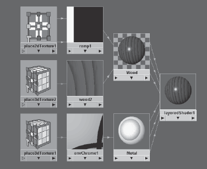
Right-click it and select Graph Network to see all the nodes of the Layered shader (shown here).
Select the axe handle geometry and then Shift+click the texture node wood2node in the Hypershade.
Choose Edit → Convert to File Texture (Maya Software)


Notice that the 3dplacement node, as well as the Hypershade view, is removed from the scene. Your axe handle's texture will now stick to the handle as a mapped-file texture.
UV mapping places the texture directly on the surface and uses the surface coordinates for its positioning. In this case, you must do a lot of work to line up the UVs on the surface to make sure the created images line up properly. What follows is a brief summary of how UV mapping works. You will get hands-on experience with UV layout with the Red Wagon later in this chapter.
Just as 3D space is based on coordinates in XYZ, surfaces have coordinates denoted by U and V values along a 2D coordinate system for width and height. The UV value helps a texture position itself on the surface. The U and V values range from 0 to 1, with (0,0) UV being the origin point of the surface.
Maya creates UVs for primitive surfaces automatically, but frequently you need to edit UVs for proper texture placement, particularly on polygonal meshes once you have edited them. In some instances, placing textures on a poly mesh will require projecting the textures onto the mesh because the poly UVs may not line up as expected once the mesh has been edited. See the next section, "Using Projections."

If the placement of your texture or image is not quite right, simply use the 2D placement node of the texture node to position it properly. See the section "Texture Nodes" later in this chapter for more information.
You need to place textures on the surface. You can often do so using UV placement, but some textures need to be projected onto the surface. It is common to project textures (when texturing polys, for example). A projection is what it sounds like. The file image, ramp, or other texture being used can be "beamed" onto the object in several ways.
You can create any texture node as either a normal UV map or a projected texture. In the Create Render Node window, select the method—Normal (for UV mapping) or As Projection—by clicking the appropriate radio button before you create the texture. (See Figure 7.29).
When you create a projected texture, a new node is attached to the texture node. This projection node controls the method of projection with an attached 3D placement node, which you saw in the Axe exercise. Select the projection node to set the type of projection in the Attribute Editor. (See Figure 7.30.)
Setting the projection type will allow you to project an image or a texture without having it warp and distort, depending on the model you are mapping. For example, a planar projection on a sphere will warp the edges of the image as they stretch into infinity on the sides of the sphere.
- Try This
In a new scene, create a NURBS sphere and a NURBS cone and place them side by side. Create a Blinn shader and assign it to both objects. In the Blinn shader's Attribute Editor, set its Color attribute to a checkerboard pattern. Make sure Normal is checked to create a UV-mapped checker texture, as shown in Figure 7.31.
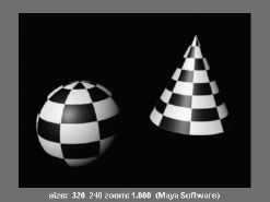
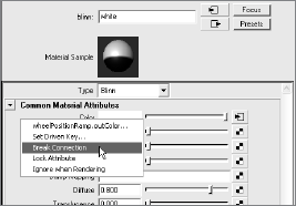
Now try removing the color map from the Blinn shader. In the Blinn shader's Attribute Editor, right-click and hold the attribute's title word Color, and then choose Break Connection from the shortcut menu. This severs the connection to the checker and resets the color to gray. Now re-create a new checker map for the color, but this time create it as a projection. In the illustration on the left in Figure 7.32, you see the perspective view in Texture mode (press the 6 key) with the two objects and the planar projection placement node.
Try moving the planar placement object around in the scene to see how the texture maps itself to the objects. Figure 7.32 on the right shows the rendered objects.
Try the other projection types to see how they affect the texture being mapped.


Projection placement nodes control how the projection maps its image or texture onto the surface. Using a NURBS sphere with a spherical projected checker, with U and V wrap turned off on the checker texture, you can see how manipulating the place3dTexture node affects the texture.
In addition to the Move, Rotate, and Scale tools, you can use the Special Manipulator tool (press T to activate or click the Show Manipulator Tool icon in the toolbar) to adjust the placement. Figure 7.33 shows this tool for a spherical projection.
Drag the handles on the special manipulator to change the coverage of the projection, orientation, size, and so forth. All projection types have special manipulators. Figure 7.34 shows the special manipulator wrapping the checker in a thin band all the way around the sphere.

Figure 7.34. The manipulator wrapping the Checker texture around the sphere (left, perspective view; right, rendered view)
To summarize, projection textures depend on a projector node to position the texture onto the geometry.
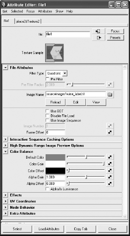
You can create a number of texture nodes in Maya. This section covers the most important. All texture nodes, however, have common attributes that affect their final look. Open the Attribute Editor for any texture node. (See Figure 7.35.) The two top sections affect the color balance of the texture. The Color Balance and Effects sections are described here.

- Color Balance
This set of attributes adjusts the overall brightness and color balance of your texture. Use these attributes to tint or brighten a texture without having to change all the individual attributes of the shader itself.
- Effects
You can invert the texture's color space by clicking the Invert check box. This changes black to white and white to black in addition to inverting the RGB values of colors.
You can map textures to almost any shader attribute for detail. Even the tiniest amount of texture on a surface's bump, specular, or color increases its realism.
2D texture nodes come with a 2D placement node that controls their repetition, rotation, size, offset, and so on. Adjust the setting in this node of your 2D texture in the Attribute Editor, as shown in Figure 7.36, to position it within the Shader network. You used a similar approach when dealing with the wood's 3D placement node in the Axe exercise earlier this chapter.
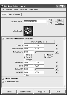
The Repeat UV setting controls how many times the texture is repeated on whatever shader attribute it is connected to, such as color. The higher the wrap values, the smaller the texture will appear but the more times it will appear on the surface.
The Wrap U and Wrap V check boxes allow the texture to wrap around the edges of their limits to repeat. When they are turned off, the texture will appear only once and the rest of the surface will be the color of the Default Color attribute found in the texture node itself.
The Mirror U and Mirror V settings allow the texture to mirror itself when it repeats. The Coverage, Translate Frame, and Rotate Frame settings control where the image is mapped. They are useful for positioning a digital image or a scanned picture.
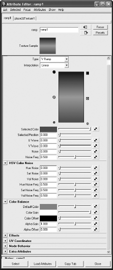
A ramp is a gradient in which one color transitions into the next color. You've already seen how useful it can be in positioning materials in a Layered shader. It's also perfect for making color gradients, as shown in Figure 7.37.
Use the round handles to select the color and to move it up and down the ramp. The square handle to the right deletes the color. To create a new color, click inside the ramp itself.
Note
The Ramp texture is different from the Ramp shader. The Ramp shader automatically has several Ramp textures mapped to some of its attributes.
The Type setting allows you to create a gradient running along the U or V direction of the surface, as well as make circular, radial, diagonal, and other types of gradients. The Interpolation setting controls how the colors grade from one to the next.
The U Wave and V Wave attributes let you add a squiggle to the U or V coordinate of the ramp, and the Noise and Noise Freq (frequency) attributes specify randomness to the placement of the ramp colors throughout the surface.
Using the HSV Color Noise attributes, you can specify random noise patterns of Hue, Saturation, and Value to add some interest to your texture. The HSV Noise options are great for making your shader just a bit different, to enhance its look.
These textures are used to create a random noise pattern to add to an object's Color, Transparency, or any other shader attribute. For example, when creating a surface, you'll almost always want to add a little dirt or a few surface blemishes to the shader to make the object look less CG. These textures are commonly used for creating bump maps.
These textures help create surface features when used on a shader's Bump Mapping attribute. Each creates an interesting pattern to add to a surface to create tactile detail, but you can also use them to create color or specular irregularities.
When used as a texture for a bump, grid is useful for creating the spacing between tiles, cloth is perfect for clothing, and checker is good for rubber grips. Placing a Water texture on a slight reflection makes for a nice poolside reflection in patio furniture.
You use the file node to import image files into Maya for texturing. For instance, if you want to texture a CG face with a digital picture of your own face, you can use the file node to import a Maya-supported image file.
To attach an image to the Color attribute of a Lambert shader for example, follow these steps:
Create the Lambert shader. (Phong, Blinn, or any of the shaders will do.)
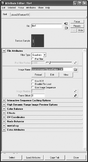
Click the Map button to map a texture on the Color attribute of the new Lambert shader. Select the file node as a normal texture. (You can also use a projected texture with an image file.) The Attribute Editor will show the attribute for the file node. See Figure 7.38.
Next to the Image Name attribute, click the Folder icon to open the file browser. Find the image file of choice on your computer. (It's best to put images to use as textures in the Sourceimages folder of the project. As a matter of fact, the file browser will default directly to the Sourceimages folder of your current project.) Double-click the file to load it.
After you import the image file, it connects to the Color attribute of that shader and also automatically connects the alpha to "transparency" if there is an alpha channel in the image. You can position it as you please by using its Place2dTexture node, or by manipulating the projection node if you created the File texture node as a projection.
You can attach an image file to any attribute of a shader that is mappable, meaning it is able to accept a texture node. Frequently, image files are used for the color of a shader as well as for bump and transparency maps. You can replace the image file by double-clicking the File texture node in the Hypershade and choosing another image file with the file browser. Maya disconnects the current image file and connects the new file.
Maya can also use Adobe Photoshop PSD files as image files in creating Shading networks. The advantage to using PSD files is that you can specify the layers within the Photoshop file to different attributes of the shader as opposed to importing several image files to map onto each shader attribute separately. This, of course, requires a modest knowledge of Photoshop and some experience with Maya shading. As you learn how to shade with Maya, you will come to appreciate the enhancements inherent in using Photoshop networks.
- Try This
You will create a single Photoshop file that will shade this sphere with color as well as transparency and a bump. Again, this is instead of creating three different image files (such as TIFFs) for each of those shading attributes.
Create a NURBS sphere in a new scene, and assign a new Lambert shader to it. You can do this through the Hypershade or the Multilister, or by choosing Lighting/Shading → Assign New Material → Lambert in the Rendering menu set. This creates a new shader and assigns it to the selection, in this case your sphere.
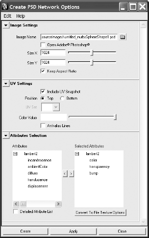
Select the sphere, and choose Texturing → Create PSD Network. In the option box that opens, select color, transparency, and bump from the list of attributes on the left side and click the right arrow to move them to the Selected Attributes list on the right, as shown in Figure 7.39.
Select a location and filename for the image. By default, Maya will place the PSD file it generates under the Sourceimages folder of your current project, named after the surface it to which it applies. Click Create.
In Photoshop, open the newly created PSD file and you'll see three layers grouped under three folders named after the shader attributes you selected when creating the PSD file. There will be a folder for lambert2.bump, lambert2.transparency, and lambert2.color, as well as a layer called UVSnapShot. The UVSnapShot layer gives you a wireframe layout of the UVs on the sphere as a guideline to paint your textures. Because the sphere is an easy model, you won't need this layer, so turn it off. You will use UVSnapShots later in this chapter. You can now paint whatever image you want into each of the layers to create maps for each of the shader attributes, all in one convenient file. Save the PSD file. You can save over it or create a new filename for the painted file.
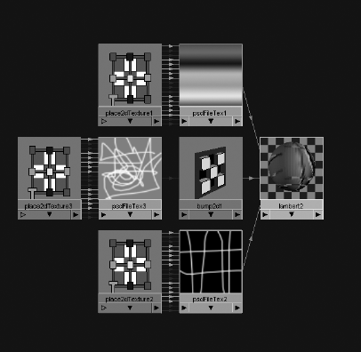
In Maya, open the Hypershade and open the Attribute Editor for the Lambert shader assigned to the sphere (in this case, Lambert2). If you graph the connections to the Lambert shader in the Hypershade windows work panel, you'll see that the PSD file you generated is already connected to the color, bump, and transparency attributes of the shader, with the proper layering all set for you as shown in Figure 7.40.
Open the file nodes for the shader and replace the PSD file with your new painted PSD file. If you saved your PSD file with the same name, all you need to do is click the Reload button to update the psdFilenode.
If you decide that you need another attribute added to the PSD file's layering, or if you need to remove an attribute, you can edit the PSD network. Select the shader in the Hypershade and choose Edit → Edit PSD Network. In the Options window, you can select new attributes to assign to the PSD file, or you can remove existing attributes and their corresponding Photoshop layer groups. Once you click Apply or Edit, Maya saves over the PSD file with the new layout.
As you saw earlier with the axe, 3D textures are projected within a 3D space. These textures are great for objects that need to reflect an environment, for example.
Instead of simply applying the texture to the plane of the surface as 2D textures do, 3D textures create an area in which the shader is affected. As an object moves through a scene with a 3D placement node, its shader looks as if it swims, unless that placement node is parented or constrained to that object, as you saw with the wooden handle of the axe. (For more on constraints, see Chapter 9, "More Animation!")
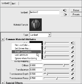
Sometimes the texture you've applied to an object is not what you want and you need to remove it from the shader. To do so, double-click the shader in the Hypershade to open its Attribute Editor.
You can then disconnect an image file, or any other texture node from the shader's attribute, by right-clicking the attribute's name in the Attribute Editor and choosing Break Connection from the context menu as shown in Figure 7.41.
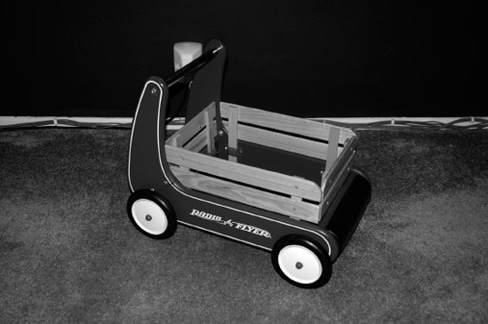
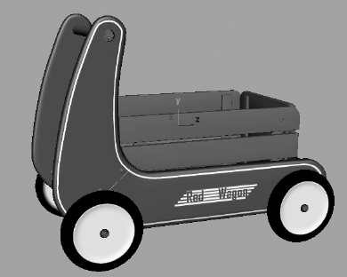
Using the model from Chapter 6, you will now assign shaders to the Red Wagon to ready the scene for lighting in Chapter 10. Later on, you will light and render the scene (in Chapter 10 and Chapter 11, respectively) to resemble the real Red Wagon shown in Figure 7.42. Take a good look at the image of the toy wagon in the Color Section of the book to see how the Red Wagon is colored. The wagon is fairly simple; it will need a few colored shaders (Red, Black, Blue and White) for the body, along with a few texture maps for the decals. The wagon will also need some more intricate work on the shaders and textures for the wood railings and silver metal screws, bolts, and handlebar that will be a good foray into image maps and UVs.
Note
This exercise is a prime example of how lighting and shading go hand in hand.
Load the file RedWagonModel_v08.ma from the Scenes folder of the RedWagon project to begin shading the finished model of the wagon.
Note
Shading is the common term for adding shaders to an object.
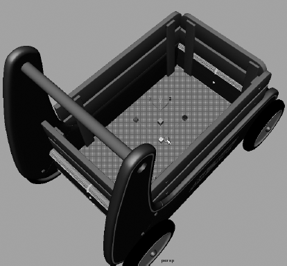
If perhaps you skipped Chapter 6—or haven't memorized that entire chapter yet—and are not familiar with this model, take a few moments to familiarize yourself with the geometry in the wagon and how it is modeled. Study the color images of the wagon and see how light reflects off its plastic, metal, and wood surfaces. Blinn shaders will be perfect for nearly all the parts of the wagon.
Open the Hypershade window, and create four Blinn shaders.
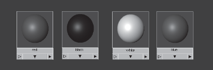
Assign the following RGB values to the Color attribute of each Blinn shader, and name them as shown in Table 7.1 and in Figure 7.43. You will create the Chrome Metal and Wood shaders later.
Table 7.1. HSV Color Values for the wagon's colors
Wagon Color | Shader Name | H Value | S Value | V Value |
|---|---|---|---|---|
Red | red | 355 | 0.910 | 0.650 |
Black | black | 0 | 0 | 0 |
White | white | 0 | 0 | 1 |
Blue | blue | 220 | 0.775 | 0.560 |
Take a look at the photo of the wagon in the Color Section in the middle of this book. The bullnose and tires are black, the wheel rims are white, the floor is blue, the screws and bolts and handlebar are chrome metal, the railings are wood, and the main body is red. Assign shaders to the wagon according to the color photo and the following steps:
In the view panel, select the side panels (the A and B panels, without the screws and bolts) and the wheel rim caps as shown in Figure 7.44, and assign the red Blinn shader to them. Press 6 to enter into Texture Display mode.
Select the wheelMesh objects for all four wheels and assign them the White shader. The tires will also turn white, but we will fix that in just a little bit, so don't worry about it now. See Figure 7.45.
Select the bullnose (the rounded cylinder in front of the wagon) and assign it the black Blinn.
Select the wagon floor object and assign it the Red shader, as shown in Figure 7.46. You'll notice that the front and back body of the wagon turn red as they are supposed to, but so does the floor of the wagon, which should be blue according to the photo in the Color Section. If you try to assign the Blue shader to the wagon floor mesh, the floor will be correct, but the front and back body of the wagon will be blue and not red. We will fix this later.


Now we have initial assignments for the basic colors of the wagon's body. Let's tweak these shaders' colors next.
Refer to Figure 7.47 to observe how the materials are different between the rim and the tire for the wheels. The rim is glossier and has a tighter, sharper specular, while the tire has a very diffuse specular and is quite bumpy. As we did for the Axe exercise, we will create a Layered shader for the wheels with white feeding into the rim portion and black into the tire.

First, we need to determine where the white ends and the black starts on the surface of the wheel mesh.
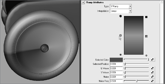
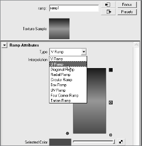
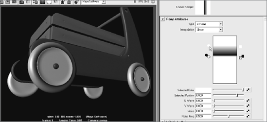
Select the White shader in the Hypershade window. Click the Map button (

The ramp is running the wrong way; we need the gradient to run from the center to the edge, and not clockwise across the wheel. In the Ramp texture's Attribute Editor, set the Type to U Ramp as shown in Figure 7.49.
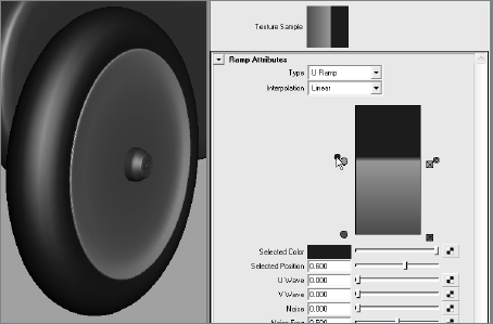
Now the color gradient should be running from the center (red) to the outside edge (green) to blue on the reverse side of the wheel. Move the blue ramp's handle in the ramp's Attribute Editor until its Selected Position value is about 0.6, as shown inFigure 7.50.
Delete the red handle in the ramp by clicking on the checked box on the right of the handle. Change the blue color to black and the green color to white. Name this ramp wheelPositionRamp. Now that we have pinpointed where the white rim ends and the black tire begins, we will use this ramp to place the Tire shader on top of the Rim shader in the Layered shader that we will eventually create.
We do not need this Ramp shader on the color of the shader anymore—we did this so we could easily see the ramp color positions in the view panels. In the Hypershade, select the White shader and click the Input and Output Connections icon (

In the Attribute Editor, RMB+click on the Color attribute and select Break Connection from the context menu to disconnect the ramp from the color. (See Figure 7.52.) Set the Color back to white. Notice that the link connecting the Ramp texture node to the White shader node disappears in the Hypershade window.
Create a Layered shader. MMB+drag the White shader from the Hypershade to the Layered Shader Attributes window, as shown in Figure 7.53. Delete the default Green shader in the Attribute Editor by clicking the checked box below its swatch.
Create a new Blinn shader, and set its color to black. Name the shader tireShader. Select the Layered Shader and then MMB+drag the new tireShader from the Hypershade to the Layered Shader's Attribute Editor, placing it to the left of the White shader, as shown in Figure 7.54. Name the Layered Shader wheelShader.
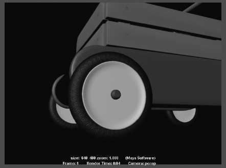
Select the wheels and assign the wheelShader Layered shader to them. The wheels should turn gray in your view panels. Layered shaders typically do not display in panels, so you will have to render a test frame. Render the persp panel, and your tire should look all white (except for the red cap). This is where the ramp we created earlier (wheelPositionRamp) comes into play. Figure 7.55 shows the all-white wheels.
Select the wheelShader, and click Input and Output Connections to graph the network in the Work Area of the Hypershade window. In the top panel of the Hypershade, click the Texture tab to display the texture nodes in the scene.
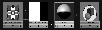
In the wheelShader's Attribute Editor, click on the tireShader swatch. MMB+drag the wheelPositionRamp node to the Transparency attribute, as shown in Figure 7.56.
Once you attach the ramp, the wheelShader icon turns white on top and black on the bottom. Render a frame in the persp panel. See Figure 7.57.
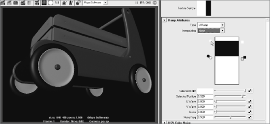
We need to add another white handle to the transparency ramp, so we can make the back rims white again. In the Hypershade, double-click the ramp to open the Attribute Editor. Add another color handle to the ramp, and set its color to white, as shown in Figure 7.58. The color of the wheel gets really weird now.
The gradient on the wheels looks wrong again. This is because the gradient in the ramp is set to linear, so the black area slowly grades to white. We need to better define that. In the ramp's Attribute Editor, set the Interpolation to None, as shown in Figure 7.59. Move that second white handle to place the white rim on the back of the wheel, and we're done coloring the wheel!


Because the material look and feel on the real wheels differs quite a bit between the rim and the tire, we will have to tweak both the White Rim shader and the Black Tire shader. Again, the rim is a smooth, glossy white, and the tire is a bumpy black with a broad specular.
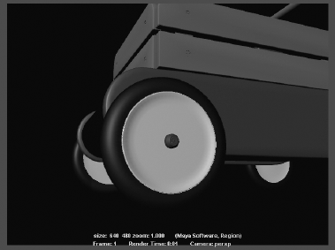
Let's set up a good angle of view for our test renders. Position your persp view to resemble the view in Figure 7.60. Render a frame.
Select the White shader and set the Eccentricity to 0.05 and the Specular Roll Off to 0.5. This will sharpen the specular highlight on the rim.
Select the black tireShader, and set the Eccentricity to 0.375 and the Specular Roll Off to 0.6 to make the highlight more diffuse across the tire. Set the Reflectivity to 0.05. Render a frame and refer to Figure 7.61.

Now let's add a bump to the Tire shader to match the feel of the tire in Figure 7.47 earlier in the chapter.

Open the Attribute Editor for the tireShader, and click the Map icon (

In the Create Render Node window, check Normal and click to create a Fractal texture map. Notice that the entire wheelShader icon becomes bumpy. (See Figure 7.62.) Render a frame, and you'll see that the entire wheel is bumpy—not just the tire! Argh!
We have to use the wheelPositionRamp to prevent the bump from showing on the rim. Select the wheelShader, and click the Input and Output Connections icon (

Note
Notice the single, blue connecting line between the fractal1 node and the bump2d1 node in the Hypershade. This means the alpha channel of the fractal feeds the amount of bump that will be rendered on the tireShader. We have to alter the alpha coming out of the fractal node with the positioning ramp to block the rim from having any bump at all. The white areas of the ramp will allow an output in alpha from the fractal, which creates a bump for the surface; whereas the black area of the ramp will keep any bump from appearing. Because we already used this ramp to position the Rim shader and the Tire shader on the wheel, it will work perfectly for the bump position as well.
Select the fractal to display it in the Attribute Editor, and MMB+drag the wheelPositionRamp in the Hypershade to the Alpha Gain attribute for the fractal, as shown in Figure 7.64.
Render a frame, and you will see that now the tire has no bump and the rim is bumpy (Figure 7.65).
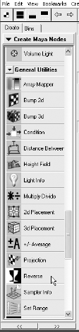
This is easy enough to fix. All we need to do is reverse the ramp and then feed it into the Alpha Gain of the fractal so that the tire is bumpy and the rim is smooth. In the Hypershade, scroll down the Create Maya Nodes pane on the left all the way down to the section heading called General Utilities. Expand it if it is closed, and click on the Reverse icon to create a reverse node in the Hypershade window. See Figure 7.66.
In the Hypershade, MMB+drag the wheelPositionRamp node onto the Reverse node and select Input from the context menu when you release the mouse button. This will connect the output of the ramp into the reverse node, which will essentially reverse the ramp.
MMB+drag the reverse node on top of the fractal1 node and select Other from the context menu. This will open the Connection Editor, which you first saw in Chapter 3 in the User Interface. On the left is loaded the reverse1 node, and on the right is the fractal1 node. In the left pane, click the plus sign next to the output entry and select output.X. In the right pane, select the alphaGain attribute, as shown in Figure 7.67.
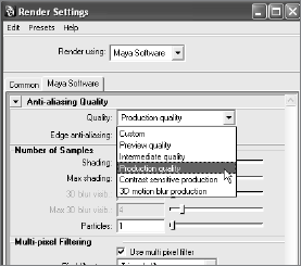
Open the Render Settings window by choosing Window → Rendering Editors → Render Settings. Click on the Maya Software tab, and set the Quality to Production Quality in the pull-down menu. (See Figure 7.68.) Render a frame, and you'll see that we finally have a bump on the tire and a smooth rim! See Figure 7.69.
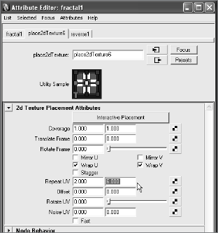
It's not a very convincing bump yet, so select the fractal node and set the Ratio to 0.85. Click the Placement tab for the fractal (it should be called something like place2dTexture6), and set the Repeat UV values to 18 and 48, as shown in Figure 7.70. This will make the fractal pattern finely speckled on the tire.
Render a frame, and the fractal's scale on the bumpy tire looks too strong. Double-click on the bump2d node in the Hypershade and, in the Attribute Editor, set the Bump Depth to 0.1. Render and check your frame against Figure 7.71. The bump looks much better, if not a little strong from this angle, but we will finesse all these settings when we render in Chapter 11. For now, it's looking pretty good!


Congratulations! You have made your first somewhat complex shading network, as shown in Figure 7.72. By now you should have a pretty good idea of how to get around the Hypershade and create shading networks. To recap, we are using a ramp to place the two Tire and Rim shaders on the wheel, as well as using it to place the bump map on just the tire by using a reverse node. The more you make these shading networks, the easier they will become to create.
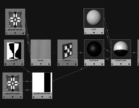
This type of shading is called procedural shading, because we used nothing but stock Maya texture nodes to accomplish what we needed for the wheels. In the following sections, we'll make good use of image mapping to create the decals for the wagon body as well as the wood for the railings.
You can load the file RedWagonTexture_v01.ma from the Scenes folder of the RedWagon project to check your work or skip to this point.
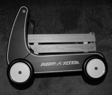
Figure 7.73 shows you the decals that need to go onto the body of the wagon. This includes the wagon's logo, which we'll replace with our own graphic design, and the white stripe that lines the side panels.
Instead of trying to make a procedural texture as we did with the wheel, we will create an image map that will texture the side panels' white stripe. The stripe is far too difficult to create otherwise. We will create an image file using Photoshop (or other such image editor) to make sure the white stripe (and later the Red Wagon logo) lines up correctly.
Mapping polygons can involve the task of defining UV coordinates for them so that you can more easily paint an image map for the mesh. When you create a NURBS surface, UV coordinates are inherent to the surface. At the origin (or the beginning) of the surface, the UV coordinate is (0,0). When the surface extends all the way to the left and all the way up, the UV coordinate is (1,1). When you paint an 800 × 600–pixel image in Photoshop, for example, it's safe to assume that the first pixel of the image (at X = 0 and Y = 0 in Photoshop) will map directly to the UV coordinate (0,0) on the NURBS surface, while the topmost right-corner pixel in the image will map to the UV (1,1) of the surface. To that end, mapping an image to a NURBS surface is fairly straightforward. The bottom of the image will map to the bottom of the surface, the top to the top, and so on. Figure 7.74 shows how an image is mapped onto a NURBS plane and a NURBS sphere.
The locations in the image, marked by text, correspond to the positions on the NURBS plane. The sphere, because it is a surface bent around spherically, shows that the origin of the UV coordinates is at the sphere's pole on the left and that the image wraps itself around it (bowing out in the middle) to meet at the seam along the front edge as shown.

Figure 7.74. An image file is mapped to a NURBS plane and a NURBS sphere. Notice the locations marked in the image and how they map to the locations on the surface, with the pixel coordinates directly corresponding to the surface's UV coordinates.
When you're creating polygons, however, this is not always the case. You sometimes will have to create your own UV coordinates on a polygonal surface to get a clean layout on which to paint in Photoshop. While poly UV mapping becomes fairly involved and complicated, it is a concept that is important to grasp early. When poly models are created, they do have UV coordinates; however, these coordinates may not be laid out in the best way for texture image manipulation.
Note
This section will assume you have some working knowledge of Adobe Photoshop. You can skip the creation of the maps and use the maps already on the CD, which are called out in the text later in the exercise.
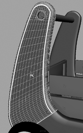
First, let's take a look at how the UVs are laid out for the A panel that we modeled first in Chapter 6.
Using your scene or the scene file
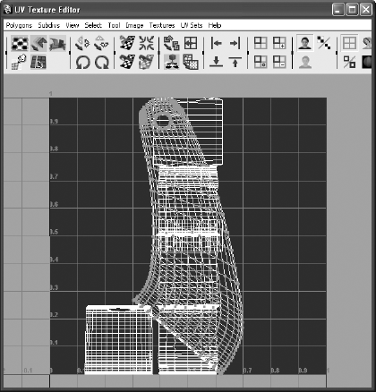
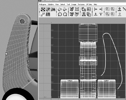
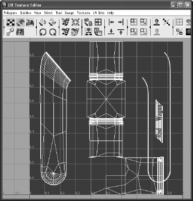
RedWagonTexture_v01.mafrom the Scenes folder of the RedWagon project, select the A panel on one side of the wagon and choose Window → UV Texture Editor, as shown in Figure 7.75.The UV Texture window works almost like any other view panel. You may navigate the window and zoom in and out using the familiar Alt + mouse button combinations.
RMB+click on any part of the wireframe layout in the UV Texture Editor window, and select UV to enter the UV selection. Select the entire wireframe mesh on the lower right, as shown in Figure 7.76. You'll notice that green points are selected—almost as if they were vertices. These are UV points and they are what define the UV coordinates on that part of the mesh. Look in the Perspective view panel and you will see the entire front face of the A panel is selected as well the green UV points (also in Figure 7.76).
Feel free to select parts of the UV layout in the UV Texture Editor to see what corresponding points appear on the mesh itself in the persp panel. This will help orient you as to how the UV layout works on this mesh.
Now we are going to again lay out just this area of the mesh's UVs. Because we already have the entire front side of the panel selected in UVs, let's convert that selection to poly faces on the model. In the Polygons menu set and in the main Maya menu bar, choose Select → Convert Selection → To Faces. Now the front faces of the A panel mesh are selected, as shown in Figure 7.77. You can always manually select just the front faces of the mesh, but this conversion method is much faster. The UV Texture Editor shows just those faces now.
With those faces selected, make sure you are in the Polygons menu set. Choose Create UVs → Planar Mapping
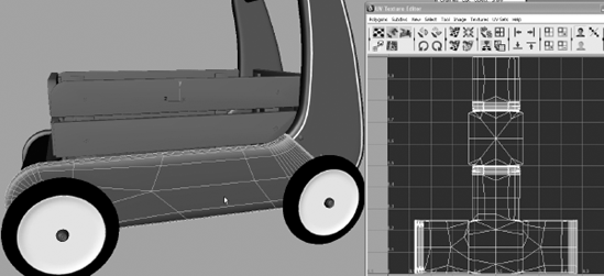
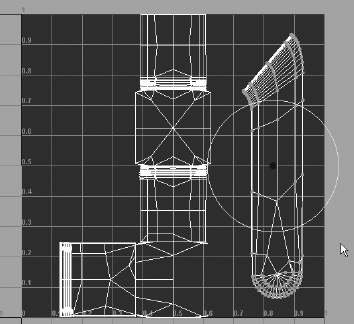
Now the front face has a much simpler UV layout from which to paint. However, it is centered in the UV Texture Editor and will overlap the other UVs of the same mesh. We should move and size it to fit into its original corner, more or less, to make sure no UVs double up on each other. In the UV Texture Editor, right-click on the wireframe and select UV to enter UV selection. Select all the UVs on those faces and you will notice that all of the UVs for the A panel mesh appear in the UV Texture Editor, and you can see the overlap. See Figure 7.79.
Press W for the Move tool, and move the selected UVs to the side of the UV Texture Editor. Press R for the Scale tool, and scale it down a bit to fit into the corner, as shown in Figure 7.80.
Earlier in the chapter, you saw how to write out a PSD file with a UV snapshot as one of its layers. We'll use a similar technique to paint the decal for the panel. Click on an empty area of the UV Texture Editor to deselect everything. Then, in Object Selection mode (press F8 if you need to exit Component Selection), select the A panel mesh in the persp panel.
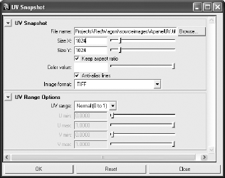
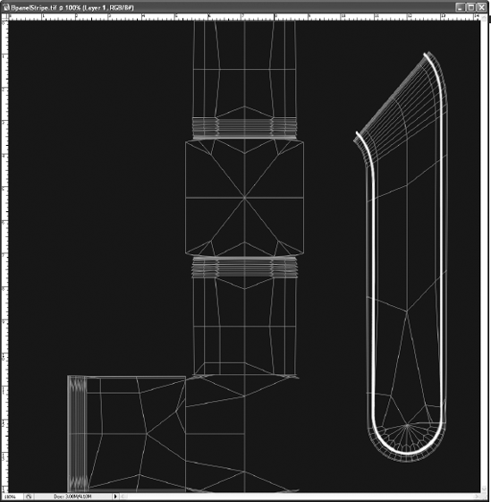
In the UV Texture Editor window, select Polygons → UV Snapshot to open the Options window. Set both Size X and Size Y to 1024. Change the image format to TIFF, then click the Browse button at the top next to File name field, and navigate to the RedWagon project's Sourceimages folder on your hard drive. Name the file ApanelUV.tif and click Save. Leave the UV range set to Normal (0 to 1) and click OK. See Figure 7.81.


Next, we'll go into Photoshop to paint our map according to the UV layout we just output.
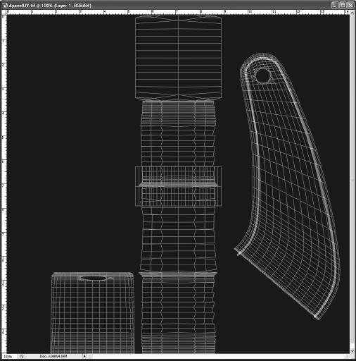
In your OS file browser, navigate to the RedWagon project's Sourceimages folder and open the file
ApanelUV.tifin Photoshop. Figure 7.82 shows the layout of the UVs that we will use to create the white stripe for the front of the A panel.In Photoshop, create a new layer on top of the background layer that is the UV layout (white on black as shown). Using the Bucket tool, fill that new layer with the same red we used on the shader in our scene. To do so, click the foreground color swatch in Photoshop and set the H to 355, S to 91 percent, and B to 65 percent, as shown in Figure 7.83. Click OK.
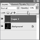
Using the Bucket tool, click to fill the entire image with the red we just created. The trouble is that now we can't see the UV layout. Set the Opacity of the red layer in Photoshop to 50 percent, as shown Figure 7.84.
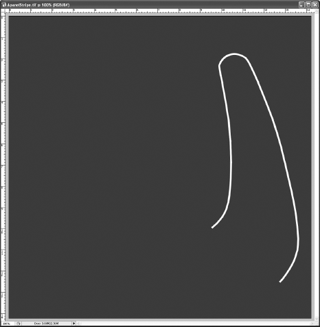
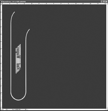
Set Photoshop's foreground color to white. Using the Line and Brush tools set to a width of about 6 pixels, draw a stripe following the UV layout lines, as shown in the image in Figure 7.85. This will place that white stripe along the A panel's outer edge because the UV lines we are following correspond to that area of the mesh. The rest will be left to be red.
You may have drawn directly on the red layer in Photoshop or created a new layer for the stripe. In either case, set the Opacity of the red layer back to 100 percent so you can no longer see the UV layout. Your image file should look like the one in Figure 7.86. Save the image as ApanelStripe.tif in the Sourceimages folder of your RedWagon project. You may keep the layers in the TIFF file, or you may choose to flatten the image or merge the layers. It might be best to keep the stripe and red on separate layers so that you can go back into Photoshop and edit the stripe as needed.


Now let's create the shader and get it assigned to the geometry.
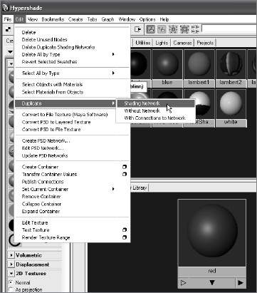
Back in Maya, open the Hypershade and select the Red shader. Duplicate it by choosing Edit → Duplicate → Shading Network in the Hypershade window, as shown in Figure 7.87.
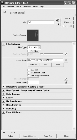
Name the new shader (called red1) ApanelStripe. Open the Attribute Editor and click on the Map button (

In the Hypershade, you might see that the Shader icon has turned somewhat transparent. Maya is automatically mapping the Transparency attribute of the shader as well as the color. Double-click the shader to open its Attribute Editor, RMB+click on Transparency, and select Break Connection from the context window, as shown in Figure 7.89. This will set the shader to the same red we used earlier, but now it will give us a stripe along the side A panel.
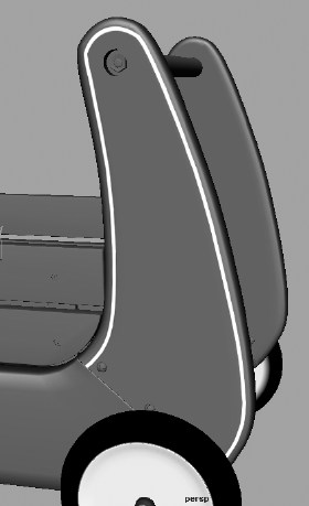
Assign the ApanelStripe shader to the A panel mesh, and press 6 for Texture Display mode in the persp panel. See Figure 7.90. The stripe lines up well.
Note
You may skip the image creation in Photoshop and use the ApanelStripe.tif image file found in the Sourceimages folder of the RedWagon project on the CD.

Now we need to put the stripe on the other side's A panel. Select the other A panel and assign the ApanelStripe shader to it. You'll notice that no stripe appears. (See Figure 7.91.) This is because the UV layout for this A panel has not been set up yet. There's no need to worry; we don't have to redo everything we did for the first A panel. We can essentially copy the UVs from the first A panel mesh to this one.
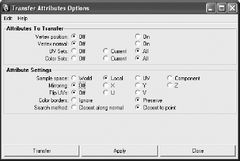
Select the first A panel (with the stripe) and the second panel (without the stripe). In the Polygons menu, set choose Mesh → Transfer Attributes
Now the stripe appears on the inside of that back A panel, and not on the outside as we need. Select that A panel and choose Modify → Center Pivot.
In the Channel box, enter a value of −1.0 for the Scale X, and the stripe will flip to the correct side, as shown in Figure 7.93.
With that A panel still selected, choose Modify → Freeze Transformations.
You can load the file RedWagonTexture_v02.ma from the Scenes folder of the RedWagon project to check your work or skip to this point.
Note
The file texture we'll use for the panels were painted in Photoshop to place the stripes and logo properly on the wagon using their UV layouts. Study the image file and see how it fits on the mesh of the wagon. Try adjusting the image file with your own art work to see how your image map affects the placement on the mesh.
With the A panels done, we'll move on to the B panels, using much the same methodology we did with the A panels. To begin, follow these steps:
Select one of the B panels, shown in Figure 7.94, and open the UV Texture Editor window.
As we did with the front face of the A panel, select the UVs on the lower-right side of the layout in the UV Texture Editor, as shown in Figure 7.95, to isolate the front face of the B panel.
Choose Select → Convert Selection → To Faces. You have isolated the front face of the B panel.
Choose Create UVs → Planar Projection
Convert the selection to UVs and use Move (W), Scale (R), and Rotate (E) to position the UV layout for that front face, as shown in Figure 7.97.
Press F8 and select the B panel mesh. In the UV Texture Editor, save a UV snapshot called BpanelUV.tif to the Sourceimages folder of the RedWagon project.
Open the
BpanelUV.tifimage in Photoshop, and follow the same steps as you did for the A panel to lay down a red layer and paint a stripe along the layout, as shown in Figure 7.98. It's best to save the stripe on its own layer in Photoshop because you will probably need to edit and reposition the stripe to make sure it lines up with the A panel stripe once you assign the shader.Create your own logo to place in the middle of panel B, and place it in the Photoshop image file, as shown in Figure 7.99. Save the image file as
BpanelStripe.tifinto the Sourceimages folder.Duplicate another Red shader and, as you did previously, assign the
BpanelStripe.tifas its color map. If needed, disconnect the transparency from the shader as you did with the A panel's shader. Name the shader BpanelStripe.Assign the BpanelStripe shader to the B panel, as shown in Figure 7.100.


Note
You may skip the image creation in Photoshop and use the BpanelStripe.tif image file found in the Sourceimages folder of the RedWagon project on the CD.

Finally, we need to create the shader for the other side's B panel. Assign the BpanelStripe shader to the other B panel. Nothing will happen because the UVs for the second B panel are not set up yet.
However, because there is a logo with text, setting up its UVs will not be as simple as copying the UVs from the first B panel and then mirroring the mesh, as we did with the A panel with a Scale X of −1.0. Doing so will make the logo and text read backward. First, let's copy and flip the UVs to the other B panel.
Select the first B panel with the correct texture, and then select the other side's B panel and choose Mesh → Transfer Attributes
We have to go back to Photoshop and create a second
BpanelStripe.tifimage file with a mirrored logo. In Photoshop, create a marquee around the logo and mirror or flip the canvas horizontally. See Figure 7.102.Select the logo portion of the image, and flip that vertically as shown in Figure 7.103. Save the image as BpanelStripe_2.tif.
Duplicate the BpanelStripe shader in the Hypershade by selecting the shader and choosing Edit → Duplicate → Shading Network. The copy is called BpanelStripe1.
Select the newly copied BpanelStripe1 shader and graph its input and output connections (

The stripe and logo are displaying on the wrong side of the B panel. Select the mesh and center its pivot.
Set the Scale X attribute for the B panel to −1.0 to mirror it. Now the stripe and logo decals will show up on the correct side of the panel. Select the mesh and freeze its transforms. Figure 7.105 shows the wagon so far.

Right now the floor of the wagon is red, like the rest of its body. However, the real wagon has a blue floor, not red. If you select the mesh for the wagon's floor (named wagonFloor) and assign the Blue shader we created, the whole body of the wagon turns blue, and that is not what we need. We only need the inside and bottom of the floor to be blue and not the front and back sides of the wagon's body.
We will make a face assignment instead of dealing with UVs and image files. RMB+click on the wagon floor mesh, and select Face from the marking menu. Select the two faces for the floor itself, as shown in Figure 7.106.
With the faces selected, assign the Blue shader from the Hypershade window and you're done! We have a blue floor. All that remains now are the screws, bolts, handle, and wood railings.
You can load the file RedWagonTexture_v03.ma from the Scenes folder of the RedWagon project to check your work or skip to this point.
We will go back to procedural shading, and use the Wood texture available in Maya to create the wood railings, as you did with the Axe exercise earlier in the chapter. Begin here:
In the Hypershade, create a new Phong material.
Click the Color Map icon (

In the Attribute Editor for the Wood texture, set the Filler Color and Vein Color attributes according to Table 7.2.
Set the Vein Spread to 0.5, Layer Size to 0.5, Randomness to 1.0, Age to 10.0, and the Grain Contrast to 0.33. In the Noise Attributes heading, set the Amplitude X to 0.2 and the Amplitude Y to 0.1 as shown in Figure 7.108. Name the shader wood.
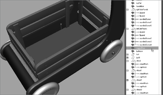
Select all the wood railings and posts, and assign the Wood shader to them. Render a frame and compare it to Figure 7.109. Notice the green cube place3dTexture node that is now in your scene. (See Figure 7.110.)
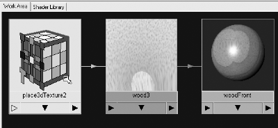
The side wood railings look fine; however, the wavy pattern on the front and back wood railings looks a bit odd. In the Hypershade, duplicate the shading network for the wood shader and call the new shader woodFront.
Assign that shader to the front and back railings and posts. Graph the network on the woodFront shader in the Hypershade window.
In the Hypershade, select the place3dTexture2 node (Figure 7.111) and the green cube in the view panels.
Rotate that placement node in the persp panel 90 degrees to the right or left. Render a frame and compare it to Figure 7.112. The wood should no longer have that awkward wavy pattern.


The wood railings are finished! Now, for some extra challenge, you can use pictures of real wood to map onto the railings for a more detailed look. The procedural Wood texture can give you only so much realism. If you create your own wood maps, use your experience with the side panels to create UV layouts for the railings so you can paint realistic wood textures using Photoshop.
Now that the railings are done and you have test renders, the black front bullnose should look pretty smooth. The actual wagon's bullnose has a texture similar to the black tires.

Select the bullnose and click Graph Materials on Selected Objects in the Hypershade (

Select the Black shader and open the Attribute Editor. Click the checkered Map button next to the Bump Mapping attribute to create a Bump map (Figure 7.113), and choose Fractal, making sure that Normal is checked.
In the Fractals place2dTexture tab, set Repeat UV to 48 and 18, as shown in Figure 7.114.
Click the bump2d node in the Hypershade and set the Bump Depth to 0.030. Render a view of the bullnose, and you should have a nice, subtle bump as shown in Figure 7.115.

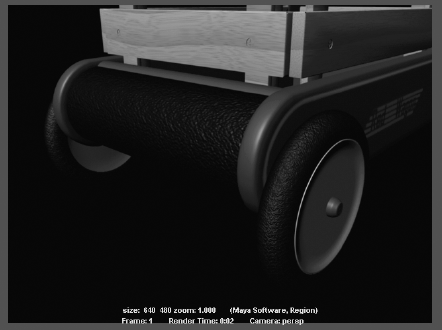
Now we'll create a simple Metal shader for the screws, bolts, and handlebar for the wagon, as we did for the Axe exercise earlier in the chapter.
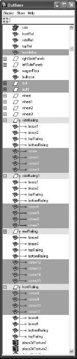
Figure 7.116. Select all the metal screws, the bolts, and handlebar and assign the Metal shader to them.
In the Hypershade, create a new Phong shader. Click the gray color swatch in the Attribute Editor, and set the color to a blue-gray (H: 207, S: 0.085, and V: 0.80). Name the shader metal.
Set the Specular Color to H: 208, S: 0.20, and V: 0.90. Set the Cosine Power to 8.0.
Set the Diffuse value to 0.2. This makes the shader appear very dark, but that's OK for now. We will finish setting up the values for the Metal shader in Chapter 10 and further refine it in Chapter 11 when we render the wagon.
In the Outliner, select all the screws, the bolts, and the handlebar and assign the Metal shader to them. See Figure 7.116.
Because metal is a tricky material to render, and a lot of metal's look is derived from reflections, we will finish setting the Metal shader's attributes in Chapter 11 when we render the wagon. We will enable raytracing to get realistic reflections and gauge how to best set up the Metal shader for a great look.
Figure 7.117 shows the wagon with all its parts assigned to shaders. Figure 7.118 shows a quick render of the wagon as it is now.
You can load the file RedWagonTexture_v04.ma from the Scenes folder of the RedWagon project to check your work or skip to this point.
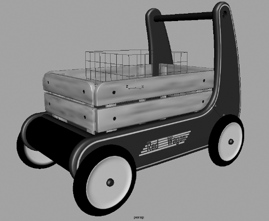

For a challenge and more experience, create new image maps for the wagon and try out your own designs. As previously suggested, you can try to create more realistic wood maps for the wagon's railings. As we continue in Chapter 10, you will begin to see how shading and rendering go hand in hand; you'll adjust many of the shaders' attributes you created in this chapter to render a stunning wagon.
You can also try to create textures to map onto the hand model you created in Chapter 4 using photos of your own hand with extensive UV manipulation.
In this chapter, you learned about the types of shaders and how they work. Each shader has a set of attributes that give material definition, and each attribute has a different effect on how a model looks.
To gain practice, you textured a NURBS axe model using various shaders, including the Layered shader, to create a wooden handle with a metal spike tip.
Next, you learned about the methods you can use to project textures onto a surface and how you can bake these projections onto an object to avoid "swimming." You learned about Maya's texture nodes, including PSD networks and the basics of UVs, and how to use them to place images onto your wagon model in a fairly detailed exercise exposing you to manipulating UVs and using Photoshop to create maps.
Texturing a scene is never an isolated process. Making textures work involves render settings, lighting, and even geometry manipulation and creation. Your work in this chapter will be expanded in Chapters 10 and 11 with discussions of lighting and rendering.
Just like everything else in Maya, it's all about collaboration—the more experience you gain, the more you'll see how everything intertwines.
However, for Maya to be an effective tool for you, it's important to have a clear understanding of the look you want for your CG. This involves plenty of research into your project, downloading heaps of images to use as references, and a good measure of trial and error.
The single best weapon in your texturing arsenal, and indeed in all aspects of CG art, is your eye, your observations of the world around you, and how they relate to the world you're creating in CG.