
CHAPTER 5
Intelligent Shoes for Human–Computer Interface1
5.1 INTRODUCTION
Recently, much research in the integration of computing and sensor technologies into human clothing has been initiated. Nonetheless, one area of wearable devices has remained relatively unexplored. This is the design and implementation of sensor- and computer-equipped intelligent shoes. Some work for human gait has focused on foot parameter detection, such as temperature, humidity, heel-off time, gait velocity, and so on. There has been little work in analyzing the foot signal despite a lot of useful data that can be extracted from the shoe. The on-going miniaturization revolution in electronics, sensor, and battery technologies, driven largely by the cell phone and handheld device markets, has made possible an intelligent shoe implementation. Along with these hardware advances, progress in human data modeling and machine learning algorithms have also made possible the analysis and interpretation of complex, multichannel sensor data.
The data glove [1], a standard input device in virtual reality applications, is used for capturing finger and wrist motion. It interprets data from different sensors and lets the user be involved in a virtual environment. Hand motion is much more investigated than foot motion in that human hands are more flexible and can perform more complicated operations.
Inspired by the successful applications of the data glove, we now investigate the possible applications of a shoe-based sensor interface. Much useful data exists that can be extracted from the shoe, especially information regarding motion when people perform different actions such as walking, standing, running, loading, and unloading. By analyzing the information given by the sensors inside the shoes, we can interpret the status of a person by his feet.
Some initial intelligent shoe systems have been prototyped. In particular, Morley et al. [12] have developed an electronic system for a shoe that monitors temperature, pressure, and humidity; however, only a hardware design is presented and there is no discussion on how the collected data are analyzed. Skelly and Chizeck [3] have presented a rule-based gait event detector with fuzzy logic and have concluded that two force sensitive resistors (FSRs) per insole are sufficient for gait event detection during walking. However, the robustness to nonwalking activities (shifting the weight from one leg to the other) is questionable. Williamson and Andrews [4] have reported excellent detection reliability by using three accelerometers attached to the shank and a machine-learning algorithm to detect the transitions among five gait phases during walking in real time, but no results have been presented for the use of this system with an functional electrical stimulation (FES) system. The Salisbury Group (U.K.) [5] has administered to several hundred patients the Odstock Dropped Foot Stimulator (ODFS). The foot switch indicates the heel-off and the heel-strike phases. The subjects learn to keep the foot switch pressed when they stop walking in order to avoid false stimulation triggers.
Moreover, various gait systems have been built with more functions and more signals for motion research. Paradiso et al. [6] have developed a wearable computer system for digital music that consists of a pair of instrumented sneakers for interactive dancing. In this work, the researchers created a few musical mappings with the shoes for computer-augmented dance. Also, Morris and Paradiso [7] have developed a compact, wireless, and wearable sensor package that is designed to provide continuous and real-time monitoring of gait for clinical applications. Pappas et al. [8] have proposed to analyze human gait patterns by using sensors attached to shoes; their system can distinguish walking from loading, unloading, or sliding of the foot. Finally, Kale et al. [9] have introduced a view-based system to recognize humans based on their gait. A hidden Markov model is used to capture the gait information in a high-dimensional image feature. Many researchers have analyzed foot motion through a set of heuristic rules. This approach, however, is only effective for simple motion patterns. Moreover, action recognition is typically based only around that of the simple motions of single individuals.
In this chapter, we develop the sensor-integrated shoe as an information acquisition platform to sense foot motion. The system is small, portable, and wearable. First, we integrated all the sensors and circuits fully inside the shoe without adding much weight into the original shoe. It is easy to use, and users will notice little difference between their normal shoes and the proposed shoes. Second, we built a hardware platform to collect data from the shoe. This platform is programmable, easily scalable, and easy to be integrated to the other applications. The platform is mainly composed of four parts, including a sensing module, a computing module, a wireless communications module, and a data visualization module. Based on this platform, we develop a novel input device called the Shoe-Mouse, which can be used by people who have difficulties in using their hands to operate computers or devices. We applied the intelligent shoes to three successful tasks, including the Shoe-Mouse, plantar pressure measurement, and human identification. Details of the application performance can be found in Section 5.3.
5.2 HARDWARE DESIGN
The proposed shoe-based information gathering platform consists of four subsystems. Figure 5.1 shows the architecture of our proposed platform.
Subsystem 1 is for sensing the parameters inside the shoe. A variety of sensors are installed inside the package, including force sensors, bend sensors, accelerometers, and so on. For ease of use, we limit the size of each device to as small as possible. Existing Micro ElectroMechanical Systems (MEMS) technology makes it possible to integrate all the sensors and circuits inside a small module.
Subsystem 2 is for gathering data from the sensors inside the shoe and sending the processed data to the wireless module. The processing power of the microprocessor is limited. It can only perform some simple calculations such as counting and averaging.
Subsystem 3 is for wireless communication. This communication system is composed of an emitter and a receiver. The receiver is for collecting the data from the circuit described in subsystem 2, whereas the emitter is for sending the data to the host computer for further analysis.
Subsystem 4 is for the visualization of the data. The received data are stored and displayed in real time on the screen of the host computer as a visual interface. This visual interface can be used for additional applications.
The prototype of the Intelligent Shoe is shown in Figure 5.2.
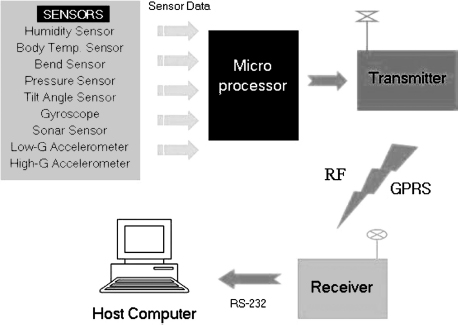
Figure 5.1. Outline of the hardware design and sensor.

Figure 5.2. The prototype of the Intelligent Shoe.
5.2.1 Sensing the Parameters Inside the Shoe
To detect the important parameters and features of gait, a variety of sensors are installed in the shoes, including force sensors, bend sensors, switch sensors, accelerometers, gyroscope sensors, and ultrasonic sensors. Existing MEMS technology makes it possible to integrate all the sensors and circuits inside a small module.
Force-sensitive resistors (FSRs) and switch sensors are selected to detect the gait timing and pressure parameters. The force sensors operate with a voltage source and a fixed resistor to produce a voltage that changes with the applied forces. Although several FSRs cannot detect force distribution of a whole foot, we can get the main force feature and gait timing parameters for identification training.
One bend sensor is selected for gait flexion detection. The bend sensor is put in the insole under the big toe and heel. The resistance of the bend sensor changes as it is bent, which can provide information about flexion between the toe and the heel. The output of the bend sensor also contains rich information about human motion, especially loading and uploading of feet.
We select three single-axis gyroscope sensors and a three-axis accelerometer to detect motion orientation of the foot. Three single-axis MEMS gyroscope sensors (ENJ-03J Murata, Murata Manufacturing Co. Ltd., Kyoto, Japan) are mounted. As a miniature vibrating-read gyro, it uses piezoelectric material to sustain vibration, while taking advantage of Coriolis forces to measure angular rate. Each gyro sensor can test one angular rate in one direction; thus, we can measure yaw, roll, and pitch of shoe motion. Also, a three-axis MEMS accelerometer (MMA7260Q Freescale Semiconductor Inc., Austin, TX) is mounted, which can detect the acceleration motion of shoe in three dimensions. The gyroscope sensors and accelerometer can detect three-dimension rotation parameters and three-dimension acceleration parameters, which can be called the inertial measurement unit (IMU).
On the other hand, one ultrasonic sensor is added to measure the height between the shoe and the ground.
5.2.2 Gathering Information from the Sensors
This subsystem is mainly composed of a processor circuit board. The original analog signal generated by the sensors is transmitted directly to the ADC channels of the micro-processor (ATMega 8535, Atmel Corporation, San Jose, CA). After A/D transform, the digital signal is passed to a wireless communication module through the transmission data (TXD) port for transmission to a PC for data analysis and visualization. A micro battery cell is also added to serve as power supply. The circuit board is small, and it can be easily put into the heel of the shoe so that users will barely notice the difference between normal shoes and intelligent shoes.
5.2.3 Wireless Communication
This subsystem is for transferring the data from the shoe to the host computer. Many foot-based gait analysis systems do not use wireless systems as these will introduce many transmission errors that make the analysis result unstable. In our system, the size of the data are relatively small and it is possible to use a wireless system. We select the GW100b wireless communication module (Unitel Pty. Ltd., Taiwan), which has a 192,000 bps transmission speed and low power consumption (less than 10 mW). With an embedded microprocessor, the GW100b can realize forward error correction (FEC), which observably reduces transmission error and improves wireless communication reliability. At the same time, with the same power consumption and error rate requirement, GW100b can transmit data for further distances with the help of the FEC rather than with other wireless communication modules without the FEC function. The wireless communication process flow is shown in Figure 5.3.
5.2.4 Data Visualization
As this platform is designed for general applications, we display all parameters measured from the shoe. The host computer gets the data from the wireless receiver via RS232. Different functions for visualizing the data from different sensors are developed and compacted. As an example, Figure 5.18 describes the real-time signals of IMU. We can also visualize a walking person by animation (in Figure 5.4), which is mapped from different gait events of the person. All of the above provide a friendly interface to display the data of the sensors obtained from the shoe.

Figure 5.3. Wireless communication process flow.
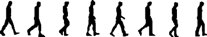
Figure 5.4. Different gait events by animation.
5.3 THREE APPLICATIONS OF THE INTELLIGENT SHOES
In the following, section we will discuss three possible applications of the intelligent shoes, including 1) intelligent shoes for human–computer interface: shoe-mouse; 2) intelligent shoes for pressure measurement; and 3) intelligent shoes for human identification.
5.3.1 Intelligent Shoes for Human–Computer Interface: Shoe-Mouse
5.3.1.1 Motivation. The Shoe-Mouse, as we call it, aims to use the shoe as a mouse to operate computers or devices. The Shoe-mounted mouse, as far as we know, has never been investigated before. One important reason is that the human foot is not as flexible as the human hand. Our motivation for creating the Shoe-Mouse comes from the following inspirations.
Including the ordinary mouse and keyboard, many input devices have been invented to help people interact with computers more easily. Most of them are used by hands and arms, which may cause injuries related to shoulders and arms after prolonged use.
Persons who have difficulties in operating computers using their hands will benefit a lot from this invention, as they can use their feet to control computers.
As we can see from the principle of other devices such as the ordinary mouse and the data glove, information of motion can be applied to map the intention of humans to the computer. Thus, we think that by integrating our developed platform for modeling the motion of the foot, it is possible to gather information from the shoe as a mouse.
5.3.1.2 Analysis of Signals from Sensors Inside the Shoe. Six parameters are selected and measured: 1) the force sensor installed at the toe; 2) the force sensor installed at the left side of the heel; 3) the force sensor installed at the right side of the heel; 4) the X-axis of the accelerometer at the heel; 5) the Y-axis of the accelerometer at the heel; and 6) the degree of bend from the bend sensor. Figure 5.5 shows the sample data taken from the Intelligent Shoe when a person wearing this shoe is walking at a speed of around 5 km/h.

Figure 5.5. Visulization of data.
It can be deducted from the figure that the data from the sensors can be easily mapped into the person's walking motion. It can be easily explained as follows: For time t from 0 s to 5 s, the force at the heel is about 50 units, which reflects the weight of the person, as a heavy person will have a larger weight on the heel of his shoe. For time t from 5 s to 7 s, the value of force at the heel becomes smaller than the original value, which means that a person is lifting his leg. For time t from 7 s to 9 s, the value of force at the heel returns to the original level again. At some key points, the value of the force is bigger than the original level, which shows that the person's foot is touching the ground. Other parameters, such as the force at the toe, and the values of the accelerometer sensors, can also be easily explained according to a person's motion.
5.3.1.3 Smoothing the Curve of the Data. In general, errors will be unavoidably introduced into the system. There are two kinds of errors. One is the error introduced from the wireless module, which can be improved by using more accurate modules. The other is introduced from the abnormal contact between the shoe and the human foot, which is the output of the sensors that do not reflect the person's intention and that should thus be deleted. These two errors will cause some abnormal peaks in the output waveform.
Here, exponential smoothing [7] is applied to minimize the effect of the abnormal peaks without affecting the performance.

Figure 5.6. Result of exponential smoothing.
The principle of exponential smoothing can be described as follows:
In Equations 5.1 and 5.2, S, α, and γ are the parameters to be decided by the user. y is the original data, and b is the processed result. As can be observed in Figure 5.6, the processed wave is smoothed while preserving the original basic configuration.
5.3.1.4 Mapping Motion of the Foot to the Motion of a Mouse-Cursor on the Screen. After analyzing the sensor data from the shoe and applying exponential smoothing to remove some noise, the motion of the foot can be mapped into the motion of a mouse-cursor on the screen. The motion of the user's shoe can cause the motion of the mouse-cursor on the screen.
Inspired by the ordinary mouse (used by hand), we divide the motion of the mouse into four classes: 1) the mouse movement in two dimensions, that is, the x–y position of the mouse-cursor on the screen; 2) the single click of the left button; 3) the single click of right button; and 4) the double click of the left button. Usually, the former three functions are enough to control a computer.
Based on the shoe-mounted data gathering platform, we use the following mapping methods to achieve the goals:
1. The Use of the Accelerometer to Produce a Motion of the Mouse-Cursor. The accelerometer used here (ADXL202E, Analog Devices, Norwood, MA) can output x-axis acceleration and y-axis acceleration. When the shoe is moved, the acceleration of the shoe is equivalent to that of the accelerometer. Figure 5.7 displays a sample output waveform of the x-axis acceleration when the shoe is moved back and forth according to a defined square route.

Figure 5.7. Output of x-axis acceleration when the shoe is following a rectangular route on a plane.
The output waveform of x-axis acceleration when the shoe is moving can be observed in Figure 5.8. It is difficult to use this signal to map the motion of the foot to the motion of the mouse-cursor. Fortunately, ADXL202E can sense the tilt angle in two directions. By using these data, we can easily map the motion of the foot into the motion of a mouse-icon on the screen. Figure 5.8 displays the output of the waveform of the x-axis and y-axis acceleration when the shoe is moved with different tilt angles.
2. The Use of the Force Sensors at the Toe to Produce the Single Click of the Left Button. The force sensor at the toe is naturally mapped into a single click. When a user has clicked the shoe using his toe, a force will be produced from the force sensor installed between the toe and the shoe. This force will persist for about 0.5 s. The average force during this time is computed and then compared with a threshold that can be calculated from some testing samples. If the force is bigger than the threshold, the function of a single click of the left button of the mouse takes effect.

Figure 5.8. Motion of foot and its corresponding acc output.
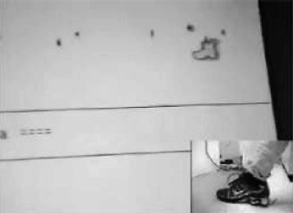
Figure 5.9. A picture captured from video demonstration.
3. The Use of the Two Force Sensors at the Heel to Produce the Single Click of the Right Button. The principle in this action is similar to that of action 2. The difference is that here we use two force sensors to judge whether the user has pressed the right button of the mouse. Simple fusion methods such as AND can be implemented in this stage. All three functions above make the control of the mouse easier. Figure 5.9 shows a picture that is captured from one of our video demonstrations.
5.3.1.5 Experiments and Performance. Two experiments were conducted to evaluate the performance of the Shoe-Mouse: 1) measurement of the force sensor installed at the toe of the shoe; and 2) measurement of the foot movement on the x–y plane to determine the trajectories of the movement as sensed by the motion sensor. The first experiment was performed to evaluate the efficiency of the left single click of the Shoe-Mouse, and the second experiment was performed to evaluate the efficiency of the movement of the Shoe-Mouse because the “Click” and the “Movement” are the two most important functions of the computer mouse.
To perform the experiments, the following items are included: 1) the subjects to perform the experiment: Three potential users were selected randomly from the lab. They were asked to perform several well-designed mouse-related actions. When performing the experiments, the subjects could see the effects of their motions on the screen. 2) A normal mouse and the Shoe-Mouse: Two kinds of mice were both tested for comparison. 3) A visualization module to calculate the efficiency of operation of the Shoe-Mouse in realtime. The following section presents the details.
1. Experimental Result of the Click Motion Test. The toe of the shoe contacts the ground with a force. By calculating the average value of this force, we can decide whether the user intends to produce a left click of the mouse. However, not all toe motions can produce the corresponding click of the mouse. We did the following experiments to evaluate the performance of the click motion.
A circle with a 30-cm diameter was drawn manually on the screen. Each of the three volunteers wearing intelligent shoes performed a simple click of a toe to produce a point in this circle. If the click is successful, it will produce a new dark point inside the circle. Finally, the number of total points was computed to evaluate the efficiency of the proposed method. Figure 5.10 shows the result of the click test. From Figure 5.10, we can see that the successful rate of clicks of a person on the average is about 0.95, which is enough for the operation of a computer.
2. Experimental Result of the Circular Motion Test. In this experiment, the motion of the shoe as it was moving around a circular path was measured. We drew a circle as a test path, letting the users draw several identical circles in the same place as accurately as they could. Then we computed the deviation between the drawn circles and the original circle. If the deviation is bigger than the threshold, we considered this circle an unsuccessful circle. After that, we compared the performance between the ordinary mouse and our proposed Shoe-Mouse. Although the performance of the ordinary mouse was a little better than the Shoe-Mouse, the Shoe-Mouse could perform ordinary tasks well enough that it can be used by a person to operate computers, especially for persons who have some difficulties in using their hands. Figure 5.11 shows the experiment and the performance. The left-most circle was drawn manually, and the middle circles were drawn by using the ordinary mouse, whereas the right-most circles were drawn using the Shoe-Mouse.
The above results show that the Shoe-Mouse can handle the operation of an ordinary mouse. It can detect the movement on the x–y plane such that it can move the cursor and handle the click motion.
5.3.2 Intelligent Shoes for Pressure Measurement
5.3.2.1 Motivation. The processing of the pressure data beneath the foot provides a specialized form of human gait analysis. Information derived from plantar pressure data can give assistance in determining and managing the impaired symptoms associated with a variety of musculoskeletal and neurologic disorders, which is of particular significance in such conditions as rheumatoid arthritis and diabetic neuropathy. Since the patients cannot sense the painful feeling of their soles correctly, the plantar pressure may be excessive. Applying the pressure higher than normal value will be an obstacle for blood reaching the tissues, which will result in ulceration, if prolonged. Based on the above reasons, different kinds of pressure measurement systems have been developed, either in the form of floor-mounted or in-shoe configuration.

Figure 5.10. Result of click test.

Figure 5.11. Performance of drawing a circle using the Shoe-Mouse.
Compared with floor-mounted systems, the in-shoe devices show more advantages. Subjects can wear the in-shoe device while walking in their normal gait without thinking about where the force platform is located. Multiple steps can be monitored by the in-shoe system but not with the force platform. Despite that the force platform system can provide both the shear and the vertical information of the ground reaction force, little loading information about the plantar surface with respect to the supporting surface is mentioned. In addition, with the development of wireless communication, the in-shoe device can be used not only in the clinic or laboratory, but also in the outdoor environment, which extends the usable locations for patients.
In the past decade, several researchers have developed in-shoe pressure measurement systems. In 1991, Hongsheng Zhu et al. developed a microprocessor-based data acquisition system to monitor the pressure distribution under seven bony prominences [10]. A wireless in-shoe force system was reported by Tracie L. Lawrence and Robert N. Schmidt in 1997 [11]. In this system, four thick-film force sensors were installed for each foot to estimate the total insole force and the center of pressure. The experiment results were compared with the Advanced Mechanical Technology, Inc., Watertown, MA (AMTI) force plate. The Pedar insole system (Novel, Munich, Germany) with 99 capacitance transducers for each insole is a commercially available system that is widely used in clinic sites and laboratories because of its repeatability and accuracy [12]. However, the limitations of this device include a heavy wireless and memory storage module, thick insole, and expensive price. The heavy weight of a wireless and memory storage module limits the period of gait trial and the applications in some violent activities, such as rapid running, dancing, jumping, and so on. Because the Pedar insole system uses the capacitance transducer, which is thicker (approximately 2 mm) in comparison with other types of sensors for in-shoe force measurement, it makes subjects feel a little uncomfortable when they wear their shoe together with this insole. The price is relatively expensive (approximately $31,000), which is unaffordable by most patients, even for some clinics.
In this part, a low-cost shoe-integrated system for measuring plantar pressure based on a support vector machine is developed. It can monitor not only the pressure distribution under the eight bony prominences but also the mean pressure beneath the entire foot. Ideal experimental results show that it is possible to use only eight FSRs to calculate the mean pressure, which used to be acquired by the device equipped with numerous sensors, such as the Pedar insole system. This intelligent system has the potential application for patients' gait analysis either in clinics or at home.
5.3.2.2 Data Acquisition. The insole subsystem shown in Figure 5.12 is a flexible instrumented part for sensing the force parameters inside the shoe. Eight FSRs (Interlink Electronics, Santa Barbara, CA) are installed on one side of a thin insole made of plastic under subcutaneous bony prominences: 1–5 metatarsal heads, hallux (big toe), and the heel (which is divided into a posterior and inside portion). Considering the different sizes of bony prominences, we select two kinds of FSRs. Two FSR-402s (12.7 mm diameter active surface, 0.5 mm thick) are used in the first metatarsal head and hallux. Six FSR-400s (5 mm diameter, 0.4 mm thick) are placed under other positions.
FSR is a type of polymer thick film (PTF) device exhibiting a decrease in resistance when an increase in the force is applied to the active area [13]. In our circuit design, a voltage divider is used to measure the resistance change of the FSR in order to obtain the relationship between the applied force and the voltage.
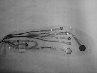
Figure 5.12. Photograph of the insole.
5.3.2.3 Sensor Calibration. To compensate the nonlinearity of FSR, each sensor needs to be calibrated after it has been located on the surface of the insole. A popular digital force gauge DPS-20 (Imada Incorporated, Northbrook, IL) is used to supply discrete force with the range from 0 kg to 10 kg for the type of FSR-400 and 0 kg to 20 kg for FSR-402. The digital outputs of force gauge are stored by PC via RS232. Then we can get the calibration result for each sensor according to the relationship between the applied force and the corresponding digital output of FSR. Experimental results demonstrate that a nine-order polynomial model provides a good fitting result. One calibration curve of FSR-402 under the first metatarsal head of right foot is displayed in Figure 5.13.
Equation 5.3 describes the relationship F between the FSR-402 output and the applied force in Newton:

where x is the digital output of FSR-402 normalized by mean 369.7 and standard deviation 223.3.
After A/D transformation, the digital data of eight FSRs are packaged, which effectively decrease the transmission error and increase the sampling frequency to 50 Hz, which is adequate for the activity of walking [14]. Then in the part of the host computer, we obtain the force information applied for each sensor based on data reconstruction and calibration. Figure 5.14, displays the pressure waveform under each region as a function of time.

Figure 5.13. One FSR-402 calibration curve.

Figure 5.14. Pressure waveforms under eight regions of right foot during normal walking (BT = hallux, M1–M5 = 1–5 metatarsal head, PH = posterior heel, and IH = inside heel).
5.3.2.4 Support Vector Regression. The feasibility of the support vector machine (SVM) in the extended application of regression problem has been proved, such as in the fields of electricity load forecasting [15], travel-time prediction [16], estimation of power system transient stability [17], and so on.
The basic idea of support vector regression (SVR) is to map a set of training points {(x1, y1), … , (xl, yl)}, (xi ∈ X ⊆ Rn, yi ∈ Y ⊆ R, l is the total number of training samples) from the input space X into a high-dimensional feature space via a nonlinear function ϕ in order that a hyperplane can be found approaching close to as many data points as possible in the feature space. SVR determines a function that can approximate future values accurately with the following linear form:
Our goal is to find a function f to minimize the regularized risk function:
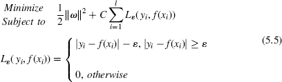
In Equation 5.3, minimizing the term ![]() ω
ω![]() 2, which is called as the regularized term, will make the function as flat as possible.
2, which is called as the regularized term, will make the function as flat as possible. ![]() representing the empirical risk is calculated by ε-insensitive loss, which is the most widely used cost function [18]. The constant C calculates the penalties to errors by determining the trade-off between the empirical risk and the regularized term. The larger the value of C is, the more penalties are assigned to errors. ε denotes the tube size of the loss function. Both parameters C and ε are selected empirically by users.
representing the empirical risk is calculated by ε-insensitive loss, which is the most widely used cost function [18]. The constant C calculates the penalties to errors by determining the trade-off between the empirical risk and the regularized term. The larger the value of C is, the more penalties are assigned to errors. ε denotes the tube size of the loss function. Both parameters C and ε are selected empirically by users.

Figure 5.15. Graphical representation for SVR.
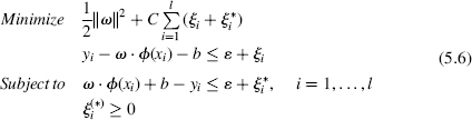
By introducing positive slack variables ξi, ξ*i used to measure errors outside the ε tube, Equation 5.5 can be transformed into the primal objective function in Equation 5.6 to cope with otherwise infeasible constraints. This situation is shown in Figure 5.15.
We construct a Lagrange function L from Equation 5.4. Then from the partial derivative of L with respect to the primal variable ω, we can get the following equation:
By substituting Equations 5.7 into 5.4, the generic equation can be rewritten as

In Equation 5.8, αi and α*i denote Lagrange multipliers satisfying positive constraints, αi × α*i = 0,αi ≥ 0. The dot product can be replaced with function K(xi, x) defined as the kernel function. The advantage of using the kernel function is that the dot product can be performed in high-dimensional feature space without having to know the nonlinear transformation ϕ(x) explicitly. Any function that satisfies Mercer's condition can be used as the kernel function. Radial basis function (RBF) kernel K(xi, xj) = exp(−γ||xi − xj||2),γ > 0 and polynomial kernel K(xi, xj) = (xi · xj + 1)d are the commonly used kernel functions for the regression problem.
We can calculate the dual variable αi, α*i by maximizing the dual problem:
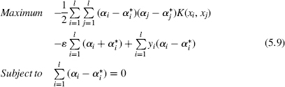
Only several nonzero Lagrange multipliers αi, α*i that fulfill the requirement can be used for the estimation of the regression line. As a remark, the sparsity of the support vector expansion is regarded because support vectors are usually a small subset of the training data points. Based on the Karush–Kuhn–Tucker (KKT) conditions [19], the constant offset b can be computed.
5.3.2.5 Experimental Results. We use SVM to train the relationship between eight FSR data and the corresponding value of mean pressure gathered by the Novel Pedar insole system mentioned above. We process the SVR experiments running the SV package LIBSVM [20]. C-SVM proposed by Vapnik and v-SVM by Schölkopf et al. [21] are two kinds of SVM algorithms used in our experiments. As mentioned in Section 3, the performances of SVMs are sensitive to the selection of kernel functions and regularization parameters. After several experimentations, we chose the RBF kernel with the parameter γ equal to 0.5 as the kernel function for both C-SVM and v-SVM algorithms based on its positive performance in nonlinear mapping compared with other kernel functions.
In the C-SVM algorithm, we mainly pay attention to the influence of the user-defined parameter C that controls the balance between model complexity and the training error. The value range of C is from 0 to infinity; however, large C will result in an overfitting problem. We list the regression results of C-SVM, respectively, when C equals 1, 10, and 30 shown in Table 5.1. It can be found that larger C corresponds to the less mean-squared error (MSE), less the number of support vectors (SVs), as well as more iterations. When C equals 30, MSE can decrease at 0.865572 after 10649 iterations. Figure 5.16 displays the comparison of prediction results in C-SVM when different values of C are selected.
The v-SVM method is a new class of SVM that is closely related to the C-SVM procedure but with a different optimization risk function. In v-SVM, the optimal separating hyperplane is obtained by solving the following minimization problem:
Table 5.1. Regression Results of C-SVM with C = 1, 10, and 30


where υ is the regularization parameter varying through [0, 1]. It limits the lower bound of the total support vectors and the upper bound number of the ones that lie on the wrong side of the hyperplane. The training of v-SVM is more intuitive in the situation of selecting the parameter υ instead of C, which may lead to the overfitting problem in C-SVM. Table 5.2 shows the regression results of v-SVM when υ equals 0.1, 0.5, and 0.8.

Figure 5.16. Comparisons of C-SVM predicted results using different parameters: (a) and (b) present the mean pressure and error when C = 1, MSE = 1.18566; (c) and (d) present the mean pressure and error when C = 10, MSE = 1.0854; (e) and (f) present the mean pressure and error when C = 30, MSE = 0.865572.
Table 5.2. Regression Results of v-SVM with υ = 0.1, 0.5, and 0.8

We compare the regression results of the two methods and find that the v-SVM algorithm is less efficient than C-SVM on the problem at hand. When υ is selected as 0.8, the MSE of v-SVM is a little more than the one of C-SVM when C equals 30. However, the value of iteration is 10 times more than the one of C-SVM. Figure 5.17 displays the prediction performance of v-SVM with υ set to 0.1, 0.5, and 0.8.
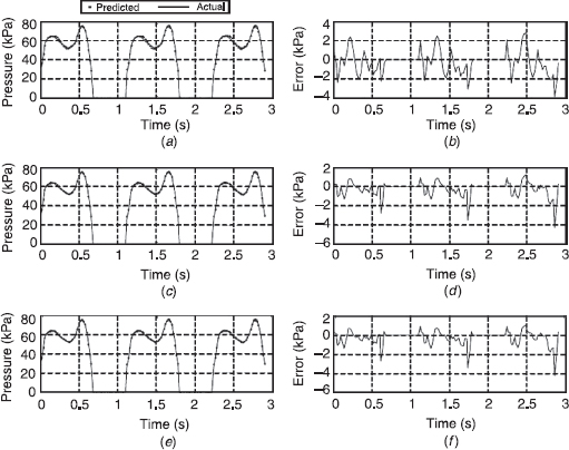
Figure 5.17. Comparisons of v-SVM predicted results using different parameters: (a) and (b) present the mean pressure and error when y = 0.1, MSE = 2.03745; (c) and (d) present the mean pressure and error when υ = 0.5, MSE = 0.929982; (e) and (f) present the mean pressure and error when υ = 0.8, MSE = 0.874932.
5.3.3 Intelligent Shoes for Human Identification
5.3.3.1 Motivation. In this part, we focus on the research of identifying individuals through their walking patterns. Each person has a unique walking style. We can sometimes even recognize our friends by only looking at their walking styles from afar, or by listening to the sound patterns they make when they walk. The unique identity of a person can be identified by analyzing his/her fingerprints, voiceprints, and/or facial features. Similarly, analyzing the way people walk, their “step-prints,” can also lead to the recognition of personal identities. Moreover, embedded force, inertial, and motion sensors in the Intelligent Shoe can offer important clues about the current activity of a user. Some previous work for human gait has mainly focused on foot parameter detection, such as temperature, humidity, heel-off time, gait velocity, and so on. As such, we propose to identify individuals by modeling their gait patterns with the integrated sensor data.
Hidden Markov models (HMMs) are doubly stochastic models and have been applied for a variety of stochastic signal processing. In speech recognition, where HMMs have found their widest application, human auditory signals are analyzed as speech patterns [22]. Transient sonar signals were classified with HMMs for ocean surveillance in Ref. 23. Radons et al. [24] analyzed a 30-electrode neuronal spike activity in a monkey's visual cortex with HMMs. Hannaford and Lee [25] classified task structure in teleoperation based on HMMs. We have previously proposed to use HMM for modeling and learning human skills. Nechyba and Xu [26] developed a validation method to compare the stochastic similarity between two dynamic, multidimensional trajectories using HMM analysis. Yang et al. applied HMMs to open-loop action skill learning [27] and to human gesture recognition [28].
The goal here is to design, build, calibrate, analyze, and use wearable intelligent shoes capable of measuring an unprecedented number of parameters relevant to gait, and to realize human identification based on gait modeling and similarity evaluation. The system is designed to collect data unobtrusively, and in any walking environment, over long periods of time. We treat gait as a human identity and a personal mark. Based on gait signal analysis, we can monitor human gait and identify the personal identity by his/her gait. A methodology based on modeling dynamic human gait and similarity evaluation with HMMs is proposed in this chapter. By achieving the modeling of human gait and physiological data, the identity of the wearer can be established through the gait pattern performance.
5.3.3.2 Data Acquisition. We select three single-axis gyroscope sensors and a three-axis accelerometer to detect the motion orientation of the foot. Three single-axis MEMS gyroscope sensors (ENJ-03J Murata) are mounted. As a miniature vibrating-read gyro, it uses piezoelectric material to sustain vibration, while taking advantage of Coriolis forces to measure angular rate. Each gyro sensor can detect the angular rate in one direction; thus, we can measure the yaw, roll, and pitch of shoe motion. Also, a three-axis MEMS accelerometer (MMA7260Q Freescale Semiconductor) is mounted, which can detect the acceleration motion of the shoes in three dimensions. The gyroscope sensors and accelerometer can detect three-dimension rotation parameters and three-dimension acceleration parameters, which can be called an IMU. We use six dynamic signals of IMU as the input signals for gait modeling and similarity evaluation.

Figure 5.18. IMU waveforms during normal walking.
After A/D transformation, the digital data of IMU is packed, which effectively decreases the transmission error and increases the sampling frequency to 50 Hz, which is adequate for the activity of walking. Then as part of the host computer, we obtain the signal information applied for each sensor based on data reconstruction and calibration. Figure 5.18 displays the waveform of IMU as a function of time.
5.3.3.3 Hidden Markov Model. In general, gait data are dynamic, nonlinear, stochastic, time-varying, noisy, and multichannel. Data will not only vary among individuals but also with a single individual over time. Moreover, decisions in motion identification cannot be made on sensor readings at a particular instance, but rather the evolution of sensor data over time must be considered. Hence, we must select a modeling framework capable of dealing with these expected complexities in the data. Based on human gait modeling, we propose to compare the overall similarity among human walking patterns of several wearers using a probabilistic model that takes the information of human walking patterns into account.
We have developed an HMM-based similarity measure to compare the similarity among different human gait models. This similarity measure is based on HMMs, which are trainable statistical models with two appealing features: (1) No a priori assumptions are made about the statistical distribution of the data to be analyzed, and (2) a degree of sequential structure can be encoded by the HMMs.
The HMM is a collection of finite states connected by transitions. Each state is characterized by two sets of probabilities: a transition probability and a discrete output probability distribution or continuous output probability density function. In each state, an output symbol will be randomly produced. The HMM λ can be specified by three matrices.
where A is the transition matrix that shows the probability of transitions among different states at any given state. B is the output probability matrix that shows the probability of producing different output symbols at any given state. π is the initial state probability distribution vector. For a given λ, it is capable of producing a series of output symbols that we call observation sequence O.
We define a stochastic similarity measure, based on discrete-output HMMs. Assume that we wish to compare observation sequences from two stochastic processes Γi and Γj. Let ![]() , denote the set of observation sequences of discrete symbols generated by process Γi. Each observation sequence is of length
, denote the set of observation sequences of discrete symbols generated by process Γi. Each observation sequence is of length ![]() , so that the total number of symbols in set Oi is given by,
, so that the total number of symbols in set Oi is given by,
The similarity measure σ between two observation sequences Oi, Oj is calculated using Equations 5.13 and 5.14, and the similarity distance measure ϕ is defined by Equation 5.15. We let Pij denote the probability of the observation sequence Oi given by the model λj, normalized with respect to Ti, the length of the sequence. In practice, Pij can be calculated using Equation 5.14 to prevent numerical underflow for long observation sequences.
Equations 5.16 to 5.18 show the properties of our similarity measure between two sequences Oi and Oj.
Given the definition of HMM, three basic problems of interest can be solved for real-world applications: the evaluation problem, the decoding problem, and the learning problem. The solutions to these three problems are the forward–backward algorithm, the Viterbi algorithm, and the Baum–Welch algorithm [29]. To develop the model state with the physical meaning of human gait, we use the Viterbi algorithm to segment the gait data sequences into states, and we study the properties of the spectral vectors that lead to the observations occurring in each state.
The human gait learning process can be connected with the similarity measure to iteratively improve a particular model. We envision that after a gait model with some stable pattern is trained, it can be stochastically perturbed in several possible directions, including structure, input representation, and choice of training data. The perturbation is parameterized into a perturbation vector Δθi, and for the original action model M(θ0) and the perturbed action model M(θ0 + Δθi) respectively, the similarity measure between the human gait data and the model-generated data is evaluated. The gradient of the similarity measure with respect to the variations in the model can be approximated and a better estimate of the motion model can be generated. Genetic approximation and simultaneously perturbed stochastic approximation (SPSA) are two techniques through which iterative model improvement can be achieved by gradient approximation. By applying the optimized action models, we believe that human gait can be identified more efficiently with lower cost and time.
5.3.3.4 Human Gait Modeling and Similarity Evaluation. In this section, we adopt HMM to account for gait modeling and similarity evaluation by modeling dynamic human gait as a separate HMM with its parameters learned from training data.
Although various types of HMMs have been proposed in the literature, we propose to apply the discrete HMM over its continuous and semicontinuous counterparts, because 1) it requires significantly less data to train reliably; 2) on average, it converges in many fewer iterations; 3) it is much less sensitive to initial random parameter settings during training; and 4) its orders of magnitude are less computationally expensive to train or evaluate. As sensor data are streamed from the intelligent shoes, it is first preprocessed through the same signal-conditioning algorithms as for the predefined gait models. The resulting observation sequence is then evaluated over the bank of gait models. Finally, the current short-term gait data are classified as that gait that has been evaluated to the highest observation probability.
We represent human gait as a time sequence. For each wearer, a separate N-state HMM will be built and the HMM training procedure will be used to optimally estimate HMM model parameters. Once the set of HMMs has been designed, optimized, and thoroughly studied, recognition of an unknown human gait is performed to score each individual gait model based on the given test observation sequence, and to select the wearer's identity whose model core is the highest matched.
1) Human Gait Modeling. We consider human gait data, including three-dimensional angular velocity and three-dimensional acceleration, as the observable stochastic process and the underlying stochastic process. Since the HMM has the ability to absorb the suboptimal characteristics within the model parameters, human dynamic gait can be represented by transition possibilities and output possibilities, and using the same model we can “learn” human identification.
For each wearer, we want to design a separate N-state HMM. Let us consider the following procedure for the modeling of human gait: 1) Represent the human gait signal of a given wearer as a time sequence of coded spectral vectors, and have a training sequence consisting of a number of repetitions of sequences of data indices of the individual gait. 2) Build individual wearer models. This task is performed by using the solution to train the HMM to optimally estimate model parameters for each model. To develop an understanding of the physical meaning of the model states, we use the Viterbi algorithm for the decoding problem to segment each training sequence into states, and then we study the properties of the spectral vectors that lead to the observations occurring in each state.
2) Similarity Evaluation. We use each set of observation sequences to train a corresponding HMM; this allows us to evaluate Pii and Pjj. We then cross-evaluate each observation sequence on the other HMM to arrive at Pij and Pji. Finally we take the ratio of these probabilities and take the square root.
To apply this similarity measure toward comparing human dynamic gait, we need to convert real-valued sensor data to a sequence of discrete symbols. The human gait data are first normalized between [−1,1]. It is then segmentized into possibly overlapping window frames. The Hamming window is applied to each frame to minimize spectral leakage caused by data windowing. The discrete Fourier transform is used to convert the real vectors to complex vectors. Using power spectral density estimation (Fourier), a feature matrix V is created. By applying Linde–Gray–Buzol (LGB) vector quantization algorithm, the feature vector V is converted to L discrete symbols such that the total distortion between the symbols and the quantized vectors can be minimized. The quantized sequence of human gait data will be used to train a six-state bakis HMM for similarity measure.
5.3.3.5 Experimental Results. In this experiment, we try to identify the person wearing the shoes by analyzing the gait performance. To estimate the gait performance by the proposed system, we invited six human subjects to wear the intelligent shoes system. These subjects are HUANG, CHA, SHI, WANG, YE, and ZHONG. Each wearer walked on flat ground under normal speed. The sampling rate was set at 50 Hz based on the gait motion frequency. The system intercepted 1800 continuous data segments (sensor data in 36 seconds) for further modeling and training.
We first employed the fast Fourier transform (FFT) technique for preprocessing the six-dimensional time sequence X(t). The Hamming window was first used with a width of 1.5 seconds (75 data segments). FFT analysis was then performed for every window, and the first three orders of FFT were kept for further precessing. After data processing, the original data matrix of size 1800 × 6 (gait data in 36 seconds) was changed to a matrix of size 75 × 18 each 1.5 seconds as one sequence for further training process. To model the human gait data X(t) = {Ax(t), Ay(t), Az(t), Gx(t), Gy(t), Gz(t)}, where A(t) represents the acceleration sensor data value of three dimensions and G(t) represents the gyroscope sensor data value of three dimensions, a discrete six-state HMM was employed to encode human gait.
For the retrieved data segments, we employed the Baum–Welch algorithm to learn 975 of the segments for the HMMs and employed the forward–backward algorithm to evaluate the other 975 data segments. The training data were divided into 13 sequences, and each sequence contained 75 data segments. We introduced six-state left–right HMMs for modeling the gait of the six wearers. We initialized all HMMs parameters using a uniform segmentation of each training data sequence. Each sequence was split into six consecutive sections, where six was the number of states in the HMM. The vectors associated with each state were used to obtain initial parameters of the state-conditional distributions.
With these initial parameters, the forward–backward algorithm was run recursively on the training data. The Baum–Welch algorithm was used iteratively to reestimate the parameters according to the forward and backward variables. Fifty iterations were run for the training processes. The forward algorithm was used for scoring each trajectory. Figure 5.19 shows all six HMMS forward scores of the results of the forward–backward algorithm, which is shown as the likelihood versus the learning iteration index.
The increase in score indicates the improvement of the model parameters. After the learning iterations, six HMMs were retrieved from the learning data samples. The HMMs λ1 to λ6 represent the human gait models from the six subjects who attended the test.
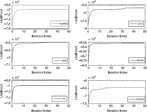
Figure 5.19. Likelihood versus Learning Iteration Index in the training process.
A) Model-to-Model Similarity Evaluation
To test and evaluate the trained models, we generated data vectors according to each given model. The data generated was the same as the training and testing set in size. Since each model represents individual gait, the HMMs λ1 to λ6, and the parameters N, M, A, B, and π were used as generators to give the observation sequence
![]()
where each observation Ok is one of the symbols from λ and M is the number of observations in the sequence, which is aforementioned as the simulated human gait data to test our models.
We used those output observations as the test input to all trained models. For each simulated observation Osim_i, where i refers to the corresponding HMM λi, forward–backward algorithm was applied to all HMMs λj (in this experiment 1 ≤ j ≤ 6). The following procedure can be used as a generator of observations:
1. Choose an initial state q1 = Si according to the initial statedistribution π.
2. Set k = 1.
3. Choose Ok = υk according to symbol probability distribution in state Si, i.e., bi(k).
4. Transit to a new state qk+1 = Sj according to the state transition probability distribution for state Si, i.e., aij.
5. Set k = k + 1; return to step (3) if k < M; otherwise terminate the procedure.
The result Pij is derived in the form of log-likelihood. In this experiment, where six human subjects were involved for testing, the complete log-likelihood is shown in Figure 5.20.
We also introduced similarity distance measure to reflect similarity evaluation. Deriving the log-likelihood P(Oi|λi) and P(Oi|λj) using the forward–backward algorithm, we obtained the similarity distance measure σ from λj to λi based on the definition of Equation 5.14. We applied the model-to-model similarity distance measure in Figure 5.21.

Figure 5.20. The likelihood of simulated sequences from HMMs to the corresponding HMMs.

Figure 5.21. The similarity distance measure of simulated sequences from HMMs to the corresponding HMMs.
To examine the results in Figure 5.20, in the ith row, the simulated test segment Osim_i generated from HMM λi is as the input to all HMMs λj for the forward–backward algorithm, and the results Pij can be seen that among all log-likelihood values for j HMMs, only when i = j, does log-likelihood achieve the maximum. In Figure 5.20, it can be clearly seen that the diagonal marked in gray achieves the maximum log-likelihood value among every single row, which can be explained as the data sequences generated from the trained models have much more similarity to the original data sequences from which the HMMs are trained than other models, or to say the HMMs are effectively to recognize similarity due to the data sequences, which is further applied to identify the wearers through their dynamic gait data sequences.
B) Human-to-Model Similarity Evaluation
To evaluate the HMMs for recognizing individual through the corresponding gait data sequences, we use the date segments, the same size as the training samples, from the testing set for individual identification. Like the procedure explained in Section 1, for each testing data sequence, we derive the log-likelihood values through the forward–backward algorithm to all trained HMMs and then the maximum log-likelihood is selected. Thus the individual identification is denoted as the corresponding HMM from which the maximum log-likelihood is derived.
We have 13 data sequences for each wearer in the test that were treated using the same preprocessing methods and have the same size. We selected two data sequences from each wearer for the identification test. The wearer's identities were counted each round, and the final results are shown in Figure 5.22. We also applied the human-to-model similarity distance measure in Figure 5.23.
C) Different HMM Structure
In the aforementioned discussion, the trained models are all based on the HMM structure of six states. We used different HMM structures and tested on the same testing data to find the best HMM structures for individual modeling method. In Figure 5.24, the testing results of average identification accuracy and the lowest identification accuracy of six wearers with different HMM structures are shown. We can see that the HMM with 9-state and 13-state can get the best performance than the other HMM structures. The average accuracy with a 9-state HMM structure is 91.03%, and the lowest accuracy is 61.54%; whereas the average accuracy with a 13-state HMM structure is 94.44%, and the lowest accuracy is 75.00%. Although 13-state corresponds to better performance than 9-state, the larger number of HMM states will increase model complexity, reduce model flexibility, and lead to overfitting in the training process. Additional explanation is required for the balance between the regularization term and the training errors. Thus, we select the 9-state HMM structure in gait modeling and identification.

Figure 5.22. The likelihood of gait sequence from individual wearer to the corresponding HMMs.

Figure 5.23. The similarity distance measure of gait sequences from individual wearer to the corresponding HMMs.
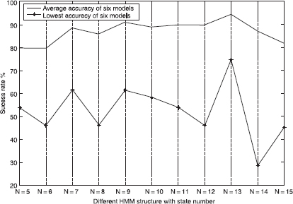
Figure 5.24. The identification success rate with gait modeling.
Furthermore, a total of 78 data segments from the six subjects were selected in the test with 9-state HMM structure, and their log-likelihoods values were derived by all trained HMMs from λ1 to λ6. The identification rate is shown in Figure 5.25.
5.4 CONCLUSION
In this chapter, we have built a shoe-based sensor-integrated platform that can gather much data inside a shoe. First, data are collected from different sensors installed in the shoe. Second, the data are computed and transmitted wirelessly to the host computer. Finally, the data are visualized on the screen. The platform is scalable and programmable. It can be used for many exciting applications such as gait recognition and human identification.
We introduced a novel input device called the Shoe-Mouse by applying the shoe platform as a user wearable interface. The Shoe-Mouse is especially designed for people who have difficulties in operating computers with their hands. As proved in the experiments, the Shoe-Mouse performs satisfactorily in motion control and can partly replace the ordinary mouse. People who do a lot of work using computers can also benefit from this invention.

Figure 5.25. The identification success rate with 9-state HMM gait modeling.
We presented a shoe-integrated plantar pressure measurement system based on the SVM to obtain the relationship between the data of eight force-sensing resistors fixed in insole and the mean pressure information gathered by the Novel Pedar insole system. Experimental results demonstrated that the regression model we built presents excellent performance of the in-shoe mean pressure prediction during the subject's normal walking. It has the potential application for aiding the patients with musculoskeletal and neurologic disorders in the development of normal gait.
We described an intelligent shoe system for collecting human dynamic gait performance. Using the proposed machine learning method HMMs, the individual wearer gait model was derived and we then demonstrated the procedure for recognizing different wearers through analyzing the corresponding models. Furthermore, we defined an HMM-based similarity measure that allows us to evaluate the resultant learning models. With the most likely performance criterion, it will help us to derive the similarity of individual behavior and corresponding model. The experimental results verify that the proposed method is valid and useful with a success human identification rate of about 91%.
REFERENCES
1. K. N. Tarchanidis and J. N. Lygouras, “Data glove with a force sensor,” IEEE Transactions on Instrumentation and Measurement, Vol. 52, No. 3, pp. 984–989, June 2003.
2. R. E. Morley, E. J. Richter, J. W. Klaesner, K. S. Maluf, and M. J. Mueller, “In-shoe multi-sensory data acquisition system,” IEEE Transactions on Biomedical Engineering, Vol. 48, No. 7, July 2001.
3. M. Skelly and H. Chizeck, “Real-time gait event detection for paraplegic FES walking,” IEEE Transactions on Systems and Rehabilitation Engineering, Vol. 9, No. 1, pp. 59–68, Mar. 2001.
4. R. Williamson, and B. Andrews, “Gait event detection for FES using accelerometers and supervised machine learning,” IEEE Transactions on Rehabilitation Engineering, Vol. 8, No.3, pp. 312–319, Sept. 2000.
5. L. Malone, C. Ellis-Hill, and I. Swain, “Using the Odstock dropped foot stimulator: user's and partner's perspectives,” in Proc. of 13th European Congress of Physical and Rehabilitation Medicine, May 2002.
6. J. Paradiso, E. Hu, and K. Y. Hsiao, “The cybershoe: A wireless multisensor interface for a dancer's feet,” in Proc. of International Dance and Technology, Tempe, AZ, 1999.
7. S.J. Morris and J. A. Paradiso, “A compact wearable sensor package for clinical gait monitoring,” Offspring, Vol. 1, No. 1, pp. 7–15, January 31, 2003.
8. I. P. Pappas, T. Keller, and M. R. Popovic, “A novel gait phase detection system,” in Proc. of Workshop Automatisierungstechnische Verfahren fur die Medizin, Darmstadt, 1999.
9. A. Kale et al., “Identification of humans using gait,” IEEE Transactions on Image Processing, Vol. 13, No. 9, pp. 1163–1173, Sep. 2004.
10. H. Zhu, G. F. Harris, J. J. Wertsch, W. J. Tompkins, and J. G. Webster, “A microprocessor-based data-acquisition system for measuring plantar pressures from ambulatory subjects,” 1EEE Transactions on Biomedical Engineering, Vol. 38, No. 7, pp. 710–714, July 1991.
11. T. L. Lawrence and R. N. Schmidt, “Wireless in-shoe force system,” in Proc. of the IEEE 19th Annual International Conference of Engineering in Medicine and Biology, Chicago, IL, pp. 2238–2241, Nov. 1997.
12. H. Hurkmans, J. Bussmann, E. Benda, J. Verhaar, and H. Stam, “Accuracy and repeatability of the pedar Mobile system in long-term vertical force measurements,” Gait and Posture, Vol. 23, No. 1, pp. 118–125, Jan. 2006.
14. T. Mittlemeier and M. Morlock, “Pressure distribution measurements in gait analysis: dependency on measurement frequency,” in Proc. of 39th Annual Meeting of the Orthopaedic Research Society, San Fransico, CA, 1993.
15. C.-C. Hsu, C.-H. Wu, S.-C. Chen, and K.-L. Peng, “Dynamically optimizing parameters in support vector regression: an application of electricity load forecasting,” in Proc. of the 39th Hawaii International Conference on System Sciences, Vol. 2, No. 7, Jan. 2006.
16. C.-H. Wu, J.-M. Ho, and D. T. Lee, “Travel-time prediction with support vector regression,” IEEE Transactions on Intelligent Transportation Systems, Vol. 5, No. 4, pp. 276–281, Dec. 2004.
17. D. H. Li and Y. J. Cao, “SOFM based support vector regression model for prediction and its application in power system transient stability forecasting,” in Proc. of IPEC 7th International Conference on Power Engineering, pp. 1–6, Nov. 2005.
18. B. Scholkopf, C. J. C. Burges, and A. J. Smola, Eds., “Using support vector machines for time series prediction,” in Advances in Kernel Methods, pp. 242–253, Cambridge, MA: MIT Press, 1999.
19. H. W. Kuhn and A. W. Tucker, “Nonlinear programming,” in Proc. of Berkeley Symp. Mathematical Statistics and Probabilistics, pp. 481–492, 1951.
20. www.csie.ntu.edu.tw/~cjlin/libsvm/.
21. B. Schölkopf, A. Smola, R. C. Williamson, and P. L. Bartlett, “New support vector algorithms,” Neural Computation, Vol. 12, pp. 1207–1245, 2000.
22. L. R. Rabiner, “A tutorial on hidden Markov models and selected applications in speech recognition,” Proc. IEEE, Vol. 77, No. 2, pp. 257–286, 1989.
23. A. Kundu, G. C. Chen, and C. E. Persons, “Transient sonar signal classification using hidden Markov models and neural nets,” IEEE Transactions on Oceanic Engineering, Vol. 19, No. 1, pp. 87–99, 1994.
24. G. Radons, J. D. Becker, B. Dulfer, and J. Kruger, “Analysis, classification and coding of multielectrode spike trains with hidden Markov models,” Biological Cybernetics, Vol. 71, No. 4, pp. 359–373, 1994.
25. B. Hannaford and P. Lee, “Hidden Markov model analysis of force/torque information in telemanipulation,” International Journal of Robotics Research, Vol. 10, No. 5, pp. 528–539, 1991.
26. M. Nechyba and Y. Xu, “Learning and transfer of human real-time control strategies,” Journal of Advanced Computational Intelligence, Vol. 1, No. 2, pp. 137–154, 1997.
27. J. Yang, Y. Xu, and C. S. Chen, “Hidden Markov model approach to skill learning and its application to telerobotics,” IEEE Transactions on Robotics and Automation, Vol. 10, No. 5, pp. 621–631, 1994.
28. J. Yang, Y. Xu, and C. S. Chen, “Human action learning via hidden Markov models,” IEEE Transactions on Systems, Man, and Cybernetics: Part A: Systems and Humans, Vol. 27, No. 1, pp. 34–44, 1997.
29. L. R. Rabiner, “A tutorial on hidden Markov models and selected applications in speech recognition,” Proc. IEEE, Vol. 77, No. 2, pp. 257–286, 1989.
1 Reprinted, by permission, from Weizhong Ye, Yangsheng Xu, and Ka Keung Lee “Shoe-Mouse: An Integrated Intelligent Shoe,” in Proc. of IEEE International Conference on Intelligent Robot and Systems, pp. 1947–1951, Edmonton, Canada, Aug. 2–6, 2005. Copyright © 2005 by IEEE; from Meng Chen, Bufu Huang, Ka Keung Lee, and Yangsheng Xu, “An Intelligent Shoe-Integrated System for Plantar Pressure Measurement,” in Proc. of the IEEE International Conference on Robotics and Biomimetics, pp. 416–421, Kunming, China, Dec. 17–20, 2006. Copyright © 2006 by IEEE; and from Bufu Huang, Meng Chen, Weizhong Ye, and Yangsheng Xu, “Intelligent Shoes for Human Identification”, in Proc. of the IEEE International Conference on Robotics and Biomimetics, pp. 601–606, Kunming, China, Dec. 17–20, 2006. Copyright © 2006 by IEEE.
Intelligent Wearable Interfaces, by Yangsheng Xu, Wen J. Li, and Ka Keung C. Lee
Copyright © 2008 John Wiley & Sons, Inc.