
6
Learning in Neuromorphic Systems

In this chapter, we address some general theoretical issues concerning synaptic plasticity as the mechanism underlying learning in neural networks, in the context of neuromorphic VLSI systems, and provide a few implementation examples to illustrate the principles. It ties to Chapters 3 and 4 on neuromorphic sensors by proposing theoretical means for utilizing events for learning. It is an interesting historical fact that when considering the problem of synaptic learning dynamics within the constraints imposed by implementation, a whole new domain of previously overlooked theoretical problems became apparent, which led to rethinking much of the conceptual underpinning of learning models. This mutual cross-fertilization of theory and neuromorphic engineering is a nice example of the heuristic value of implementations for the progress of theory.
We first discuss some general limitations arising from plausible constraints to be met by any implementable synaptic device for the working of a neural network as a memory; we then illustrate strategies to cope with such limitations, and how some of those have been translated into design principles for VLSI plastic synapses. The resulting type of Hebbian, bistable, spike-driven, stochastic synapse is then put in the specific, but wide-scope, context of associative memories based on attractor dynamics in recurrent neural networks. After briefly reviewing key theoretical concepts we discuss some frequently overlooked problems arising from the finite (actually small) neural and synaptic resources in a VLSI chip. We then illustrate two implementation examples: the first demonstrates the dynamics of memory retrieval in an attractor VLSI network and explains how a good procedure for choosing interesting regions in the network’s parameter space can be derived from the mean field theory developed for attractor network; the second is a learning experiment, in which a stream of visual stimuli (acquired in real time through a silicon retina) constitutes the input to the spiking neurons in the VLSI network, thereby driving continuously changes in the synaptic strengths and building up representations of stimuli as attractors of the network’s dynamics.
6.1 Introduction: Synaptic Connections, Memory, and Learning
Artificial neural networks can imitate several functions of the brain, ranging from sensory processing to high cognitive functions. For most of the neural network models, the function of the neural circuits is the result of complex synaptic interactions between neurons. Given that the matrix of all synaptic weights is so important, it is natural to ask: how is it generated? How can we build a neural network that implements a certain function or that imitates the activity recorded in the brain? And finally, how does the brain construct its own neural circuits? Part of the structure observed in the pattern of synaptic connections is likely to be genetically encoded. However, we know that synaptic connections are plastic and they can be modified by the neural activity. Every time we go through some new experience, we observe some specific pattern of neural activity, that in turn modifies the synaptic connections. This process is the basis of long-term memory, as the mnemonic trace of that experience is most likely retained by the modified synapses, even when the experience is over. Memories can then be reactivated at a later time by a pattern of neural activity that resembles the one that created the memory, or more in general, that is strongly affected by the synapses that have been modified when the memory was created. This form of memory is also fundamental for any learning process in which we modify our behavior on the basis of relevant past experiences.
There are several models of artificial neural networks (see, e.g., Hertz et al. 1991) that are able to learn. They can be divided into three main groups: (1) networks that are able to create representations of the statistics of the world in an autonomous way (unsupervised learning) (Hinton and Sejnowski 1999); (2) networks that can learn to perform a particular task when instructed by a teacher (supervised learning) (Anthony and Bartlett 1999); and (3) networks that can learn by a trial and error procedure (reinforcement learning Sutton and Barto 1998). These categories can have a different meaning and different nomenclature depending on the scientific community (machine learning or theoretical neuroscience). All these models rely on some form of efficient long-term memory. Building such networks in analog electronic circuits is difficult, as analog memories are usually volatile, or when they are stable the synaptic modifications can be remembered with a limited precision. In the next section we review the memory problem for neuromorphic hardware and some of the solutions proposed in the last two decades. We first discuss how memories can be retained over long timescales (memory maintenance); then we address the issue of how new memories are stored (learning) and we discuss the process of memory retrieval in binary and spiking attractor neural networks. Finally, we offer an example of memory retrieval in a neuromorphic, VLSI recurrent spiking neural network, and a simple instance of Hebbian dynamic learning in the same chips, based on the stochastic synaptic dynamics described in the previous sections.
6.2 Retaining Memories in Neuromorphic Hardware
6.2.1 The Problem of Memory Maintenance: Intuition
Highly simplified neural networks like perceptrons (Block 1962; Minsky and Papert 1969; Rosenblatt 1958) and Hopfield networks (Amit 1989; Hopfield 1982) can store and retrieve an enormous number of memories, to the point that, at the beginning of the 1990s, theoretical neuroscientists thought that the memory problem was solved. It was actually in an attempt to implement these models in neuromorphic hardware that Amit and Fusi realized in 1992 that there is a serious fundamental problem related to memory storage (Amit and Fusi 1992 1994). Models of biological synapses are inevitably highly simplified and they try to capture the features of the synaptic dynamics that are important to implement a cognitive function. Amit and Fusi realized that one of the simplifications in the previous modeling work, allowing synaptic strengths to vary in an unlimited range, has dramatic implications for the memory capacity. Networks with realistic, bounded synapses have a strongly reduced memory capacity, because old memories are overwritten by new ones at a very fast rate.
We explain this point with a simple intuitive argument (Fusi and Senn 2006). Consider a neural network that is exposed to a continuous stream of experiences that we would like to store in the memory of the synaptic weights (see Figure 6.1). We now consider one generic synapse and we focus on a particular experience whose memory we intend to track (we name it A). We first consider the case of an unbounded synapse (Figure 6.1a). The synapse starts from some initial state (we set it arbitrarily to zero), and it is modified when the network goes through each experience. For example, its efficacy is strengthened by experience A, as shown in the figure.
We now make the assumption that there is an efficient mechanism of retaining that value of the synaptic strength, at least until the occurrence of a new event that modifies it (B). The maintenance of a precise value might require complex mechanisms, as it certainly does in biological systems, but for now we ignore this issue and we assume that synaptic values can be preserved indefinitely in the absence of new events.

Figure 6.1 Limiting the synaptic strengths between two bounds causes forgetting. (a) An unbounded synapse remembers about experience A. The synaptic value is plotted against time. Every experience (A,…,F) modifies the synapse either upwards or downwards. (b) The same synapse is now bounded from above (the shaded wall represents a rigid bound for the maximal value of the synapse). The trajectories which can be seen through the wall are those that the synapse would have followed, were not bounded there. Now the modifications induced by A cannot be propagated up to the present time
The final value of the synapse will reflect the series of synaptic modifications induced by all the new events (C,D,…,F). Is the synapse still retaining any memory of A? One way to answer is to perform the following virtual experiment: we go back to the past, we modify A (A → A’), and we see whether such a modification can propagate up to the present time. For example, we change experience A in such a way that the synapse is weakened instead of being potentiated. If synaptic modifications simply add up linearly, then the trajectory representing the synaptic weight as a function of time (gray) is parallel to the first one. Obviously the final value will be different, and it will be correlated to the synaptic modification induced by A. So in principle we still have memory of what happened in A, although we might not be able to recollect all the details about the experience A. However, the important point is that the mnemonic trace is still there as the final value of the synaptic strength is correlated with the modification induced by A.
We now consider a bounded synapse (Figure 6.1b). We do exactly the same experiment as we did for the unbounded synapses. Now experience B already brings the synapse to its saturation value (indicated by a shaded wall). The synapse cannot go any further up, so it stays at the maximum, also when experience C tries to potentiate the synapse again. When we now go back to the past and modify A into A’, we see that initially the black and the gray trajectories are different, but when the synapse goes through experience C, it hits the upper bound and the two trajectories become identical. In particular, the final value will also be the same, whether the synapse went through A or A’. In this case the modification induced by A cannot affect the final synaptic value. So at the present time A has been forgotten. This simple example shows that every time the variables describing the synaptic dynamics are restricted to vary in a limited range, old memories are naturally forgotten (see also Fusi 2002; Parisi 1986).
6.2.2 The Problem of Memory Maintenance: Quantitative Analysis
Memories are naturally forgotten when the synaptic weights are restricted to vary in a limited range. How fast is such a forgetting? We can easily estimate the typical memory lifetime in a population of bistable synapses for which the lower and the upper bounds coincide with the only two stable states. This may sound as an extreme case of a bounded synapse, but it is actually representative of a wide class of realistic synapses (see Section 6.2.3). When there are only two synaptic states, every time a synapse is modified, the past is entirely forgotten. For example, if one experience wants to strengthen a synapse, then the synapse ends up in the potentiated state, whether it started from the depressed or an already potentiated state. The initial condition preceding the modification contained all the information about previously stored memories, and it is forgotten. As a consequence, every time we go through some new experience, there will be a fraction of synapses that is modified in which we store information about the new experience and we forget the other memories. The remaining synapses are left unchanged, and hence they preserve the old memories, but they do not store any information about the new experience. After experience A, which again leads to the memory that we intend to track, a number n = qN of synapses store information about A (N is the total number of synapses and q is the average fraction of modified synapses). When we go through the experiences B,C,D,…, we assume that their neural representations are random and uncorrelated. This assumption is motivated by the belief that the brain has an efficient mechanism to compress the information before it stores it. The incompressible part of the information can reasonably be modeled as some sparse patterns of random and uncorrelated activities. Indeed, were it correlated to one of the previously stored memories, it would still be compressible. We now ask ourselves: how many distinct memories can we store? We assume also that each memory is stored in a single exposure. A second exposure would be equivalent to a highly correlated memory, and we assumed that there is an efficient mechanism to deal with correlations. We will see that there is a problem of memory capacity even under all these simplifying assumptions. When the memories are random and uncorrelated, then after p experiences we have
Indeed, the tracked experience A is not special in any way, it is just the one we decided to track. Hence we should use the same rule for updating the synapses for all memories, and that is why q is always the same for every synaptic update. From the formula it is clear that n decays to zero exponentially with p. To retrieve information about the tracked memory, at least one synapse should be able to remember it (n ≥ 1). This imposes a tight constraint on the number of uncorrelated patterns p which can be stored:
![]()
The logarithmic dependence on N makes this limitation severe, and the neural network extremely inefficient as a memory. Most of the synaptic resources are devoted to the last stimuli seen, even when the information collected about the stimulus and stored in the synapses is more than what is needed to retrieve correctly the memorized pattern. Notice that the condition that at least one synapse remembers is a necessary condition. In general, it will not be sufficient to retrieve the memory, and sometimes not even to recognize it as familiar. The number of experiences p can also be regarded as the memory lifetime expressed in terms of the number of patterns whose memory trace is still in the present synaptic structure. This memory trace can be so feeble that it might be impossible to retrieve any information about the pattern of activities in the memory sliding window.
This argument, made for simplicity in the case of bistable synapses, actually applies to any realistic memory system and it can be made rigorous for a wide class of synaptic models (see Fusi 2002).
In the case of traditional neural network models, most of the synaptic models had weights that could vary in an unlimited range, or similarly, the weights could be modified with arbitrary precision. For example, in the case of the Hopfield network (Hopfield 1982) or the perceptron learning rule (Rosenblatt 1962), the range in which the synapses vary typically increases linearly with the number of stored memories. In all these cases there is no equilibrium distribution, as the distribution of synaptic weights keeps changing. At any time, the distribution is always correlated to all stored memories, and the reasons why memories cannot be retrieved are only related to the interference between different memories. In other words, the memory signal (i.e., the correlation between a synaptic matrix and a particular memory) remains constant with time, whereas the noise (i.e., its fluctuations) increases with the number of memories. In the case of the Hopfield network, the memory capacity, expressed in terms of random uncorrelated patterns that can be retrieved, grows linearly with the number of neurons, which is significantly better than the logarithmic dependence of bounded synapses, for which the memory signal decays exponentially fast, whereas the noise remains approximately constant.
It is also important to notice that the limitation due to the boundedness of the synaptic weights is not so severe in the case of off-line learning. For example, in the case of the Hopfield model, if one first computes the unbounded synaptic weights according to the Hopfield prescription, and then binarizes them, the number of retrievable patterns still scales linearly with the number of neurons (Sompolinsky 1986). However, this procedure is not possible in a physical system in which there are not temporary repositories which allow to store synaptic weights with unlimited precision.
6.2.3 Solving the Problem of Memory Maintenance
The expression of the upper bound of the number of uncorrelated patterns p suggests a possible way out to elude the memory constraint: if synaptic changes are small or rare enough (q ≪ 1), then the sliding window in which modifications are remembered can be extended by a factor 1/q:
![]()
The price to be paid by reducing the size and the number of synaptic modifications is the reduction of the initial memory trace, the one experienced immediately after the memory is stored. In other words, the amount of storable information per memory decreases whenever the synaptic model is modified to reduce q. This is a general property of any realistic synapse: as the memory lifetime is extended, the initial memory trace and hence the amount of information per memory is sacrificed to some extent. In what follows we review a few effective ways of extending memory lifetimes that are related to both the neural representation of memories and the details of the synaptic dynamics. They all affect in different ways the initial memory trace. In most of the cases, different ‘ingredients’ can be combined together to further improve the memory performance.
Extending Memory Lifetimes with Slow Stochastic Learning
The memory lifetime can also be extended by modifying a randomly selected fraction of all synapses that are eligible for a long-term change (as already discussed in the simple example of bistable synapses). Such a mechanism can be easily implemented if each synapse is modified with a given probability. This stochastic selection turns out to work nicely for random uncorrelated patterns even when the number of synaptic states is reduced to the extreme case of two (Amit and Fusi 1992, 1994; Fusi 2002; Tsodyks 1990). In the case of random uncorrelated binary patterns, if the synapses are modified with a probability q, then we have already seen that the memory trace S, defined as the fraction of synapses that are correlated with a particular tracked memory, decays as
S(p) = q(1 − q)p = qeplog(1−q)∼ qe−pq,
where p is the number of random uncorrelated memories that are stored after the tracked memory. S(p) is proportional to q, as q is the fraction of synapses that are modified for each memory, and it is multiplied by the probability that the synapse is not modified by the other p memories, which is (1 − q) to the power of p. For a small q (slow learning), the initial memory trace S(0) is also small; however, S(p) decays exponentially with a long ‘time constant’ that goes like 1/q. If q is large (fast learning), new memories are acquired rapidly because a large fraction of synapses are modified, but memories are also quickly overwritten. If q = 1 (deterministic synapses), then only one memory can be remembered (this result can be derived by using the exact expression of S(p)). When we read out N independent synapses, the fluctuations are of the order of ![]() . These fluctuations are due both to the stochastic nature of the memories and to the inherently stochastic processes underlying synaptic modifications. The signal-to-noise ratio SNR(p), defined as the expected number of synapses that remember a particular memory divided by its standard deviation, goes like
. These fluctuations are due both to the stochastic nature of the memories and to the inherently stochastic processes underlying synaptic modifications. The signal-to-noise ratio SNR(p), defined as the expected number of synapses that remember a particular memory divided by its standard deviation, goes like
![]()
If we require that SNR(p) is larger than some arbitrary value, say 1, then we have approximately
![]()
The memory capacity is again catastrophically low, as p scales logarithmically with N. If q is small, and in particular, if it is properly chosen for each given size of the network (specifically, it goes to zero as N increases), then we can extend the memory lifetime. The smallest q we can afford is ![]() (otherwise the argument of the log becomes smaller than 1 and the logarithm becomes negative), which means
(otherwise the argument of the log becomes smaller than 1 and the logarithm becomes negative), which means ![]() . For unbounded synapses we would have had p < αN, where α is a constant, so there is still a significant reduction in performance, but the improvement over the logarithmic dependence is also considerable. Stochastic learning is the most widely used solution to the memory problem in learning neuromorphic systems. See also Section 6.3 for a dynamical implementation.
. For unbounded synapses we would have had p < αN, where α is a constant, so there is still a significant reduction in performance, but the improvement over the logarithmic dependence is also considerable. Stochastic learning is the most widely used solution to the memory problem in learning neuromorphic systems. See also Section 6.3 for a dynamical implementation.
Notice that in general, slow stochastic learning is a good solution to the memory problem for any form of learning that is inherently slow. For example, reinforcement learning (Sutton and Barto 1998) is based on a trial-and-error approach that usually requires a large number of iterations before learning converges to the policy that maximizes the cumulative future reward. In this case the learning process is inherently slow, as the number of synapses that should be modified at each iteration is anyway small. In these situations the introduction of synaptic boundaries does not necessarily disrupt the memory performance of the learning system.
Extending Memory Lifetimes with Sparse Memories
If the neural representations of memories are random and sparse, i.e., with a small fraction f of active neurons, then there are situations in which the number of storable memories increases by a factor f −2(Amit and Fusi 1994; Fusi 2002). This is a consequence of the fact that the learning rule can be designed so that the probability that a single synapse is modified scales like f 2. In other words, sparsifying the neural representations is equivalent to reducing the number of synapses that are modified on average every time a new memory is stored (see also Section 6.2.3 on slow learning). Of course the amount of information that can be stored for each memory also decreases as the neural representations become sparser (it scales approximately linearly with f). If f goes to zero as the total number of synapses increases, then the memory lifetime can be extended up to O(N2) (Amit and Fusi 1994; Fusi 2002). However, this scaling is obtained for neural networks in which the number of synapses increases with the number of neurons. In more realistic situations the number of synapses per neuron is large but fixed, and in particular it does not scale with the total number of neurons. In large-scale neural systems with billions of synapses and a limited number of synapses per neuron, sparseness can increase the memory performance but only to some degree. Indeed, if one assumes that f goes to zero with the total number of synapses, then the neural representations would be required to be so sparse that it would be impossible to retrieve them (Ben Dayan Rubin and Fusi 2007). This conclusion is valid only if one assumes that the neural representations of the memories are random and uncorrelated, and that every neuron has to be able to retrieve some information about the stored memory. It is clear that these assumptions are not met in the real brain, and it is likely that there are specific neural architectures that can take advantage of sparseness in a more efficient way.
Extending Memory Lifetimes with Supervision
Consolidated synaptic modifications should be rare events in the learning process. In the unsupervised learning scenario the selection of the synapses that should be changed can be partially operated by the neural activity and partially by the inherent stochastic mechanism acting at the level of each synapse. Any kind of supervision providing some additional feedback about the correctness of the synaptic modification might help to refine the selection of the synapses to be modified. For example, the principle of the perceptron learning algorithm (Rosenblatt 1962), stating that synapses are modified only if the response of the neuron does not match the response desired by the teacher, can further reduce the average number of modified synapses without sacrificing the stored information. See Senn and Fusi (2005a, 2005b) and Fusi and Senn (2006) for a quantitative analysis of these neural systems in the case of bistable synapses. The number of storable random uncorrelated patterns goes from ![]() . However, the improvement in memory performance is significantly higher if one considers the problem of classification of correlated patterns.
. However, the improvement in memory performance is significantly higher if one considers the problem of classification of correlated patterns.
Extending Memory Lifetimes with Synaptic Complexity
So far we have considered only synapses with two stable states. How does the memory performance improve when we increase the number of synaptic states? This is a particularly important question for neuromorphic systems, as it is fundamental to know how much one should invest in the complexity of the circuits implementing each synapse.
There are many ways of increasing the complexity of a synapse. Not all of them lead to significant improvements in memory performance and it is surprising that the simplest bistable synapses are in many situations as good as more complex synapses. We will first consider what happens in the case in which each synapse has more than two states between the minimal and the maximal efficacies and then we will summarize the theoretical studies for synaptic complexity in the form of meta-plasticity.
Multistate Synapses
If we increase the number of states that each synapse has to traverse to go from the minimum to the maximum weight, we achieve a relatively small improvement. For simplicity, we consider the case in which the synapses are deterministic (the transitions between states are not stochastic). Synapses with stochastic transitions would have the same dependence on the number of states, but both the initial SNR and the memory lifetime p would be scaled by the same factor (SNR(0) → SNR(0)q, p → p/q if q is the transition probability from one state to the neighboring one). If m is the total number of synaptic states, then the memory capacity scales as shown by Amit and Fusi (1994) and Fusi and Abbott (2007):
![]()
The dependence on N is still logarithmic; however, one also gets an extra factor that is proportional to m2. The initial SNR is reduced by a factor 1/m. For small neural systems, this may be a reasonably good solution to the memory problem, but for large systems the capacity is still far from what we can achieve with stochastic learning. Indeed, in order to match the performance of bistable synapses with stochastic transitions, one would need m ∼ N1/4, which is significantly more difficult than reducing the transition probabilities to ![]() in a bistable synapse. Moreover, there is a more serious limitation to be considered. The m2 factor that extends the memory lifetime is obtained only when synaptic potentiation is perfectly balanced with synaptic depression. Otherwise there is actually no improvement at all with the number of synaptic states, and the performance is again catastrophically poor, comparable to the case of a deterministic bistable synapse (Fusi and Abbott 2007). Not surprisingly, there is accumulating evidence that biological single synaptic contacts are indeed bistable on long timescales (O’Connor et al. 2005; Petersen et al. 1998).
in a bistable synapse. Moreover, there is a more serious limitation to be considered. The m2 factor that extends the memory lifetime is obtained only when synaptic potentiation is perfectly balanced with synaptic depression. Otherwise there is actually no improvement at all with the number of synaptic states, and the performance is again catastrophically poor, comparable to the case of a deterministic bistable synapse (Fusi and Abbott 2007). Not surprisingly, there is accumulating evidence that biological single synaptic contacts are indeed bistable on long timescales (O’Connor et al. 2005; Petersen et al. 1998).
Metaplastic Synapses
Metaplastic changes are defined as long-term modifications that can affect not only the synaptic efficacy, but also the parameters that characterize the synaptic dynamics, and hence the way synapses are modified by future experiences. There is a class of metaplastic synapses that outperform other memory models by having a strong initial SNR that scales with ![]() and, at the same time, their memory lifetime scales with
and, at the same time, their memory lifetime scales with ![]() . These models are constructed on the basis of simple considerations: fast bistable synapses that operate on short timescales (q ∼ 1) are very plastic and hence good for storing new memories, but bad at retaining old ones (
. These models are constructed on the basis of simple considerations: fast bistable synapses that operate on short timescales (q ∼ 1) are very plastic and hence good for storing new memories, but bad at retaining old ones (![]() and memory lifetime p ∼ 1). On the other hand, slow synapses, operating on long timescales (q ≪ 1), are relatively rigid, and they are good for memory preservation, but bad for the storage of new memories (SNR(0) ∼ 1 and memory lifetime
and memory lifetime p ∼ 1). On the other hand, slow synapses, operating on long timescales (q ≪ 1), are relatively rigid, and they are good for memory preservation, but bad for the storage of new memories (SNR(0) ∼ 1 and memory lifetime ![]() ). Fusi et al. (2005) realized that it is possible to design a synapse that operates on multiple timescales and it is characterized by both long memory lifetimes and strong initial memory traces. The proposed synapse has a cascade of states with different levels of plasticity, connected by metaplastic states. The level of plasticity depends on the past history of synaptic modifications. In particular there are two chains of m synaptic states, corresponding to two strengths of the synaptic weights. When a synapse is modified, the synapse goes into one of the states at the top of the cascade. These states are very plastic (q = 1). If the synapse is repeatedly potentiated, then it moves down in the chain of potentiated states, and each state becomes progressively more resistant to depression (q ∼ xk, where x < 1 and k = 1, …, m). In other words, the dynamic properties of the synapse change depending on how many consecutive potentiations occur (metaplasticity). The same is valid for depressions. At equilibrium, all the metaplastic states are equally occupied. This means that there are always synapses at the top of the cascade, that are very plastic and ready to store new memories, as well as synapses that are at the bottom of the cascade and preserve consolidated remote memories. For such a synaptic model the memory trace decays as a power law on a wide range, and then it decays exponentially fast:
). Fusi et al. (2005) realized that it is possible to design a synapse that operates on multiple timescales and it is characterized by both long memory lifetimes and strong initial memory traces. The proposed synapse has a cascade of states with different levels of plasticity, connected by metaplastic states. The level of plasticity depends on the past history of synaptic modifications. In particular there are two chains of m synaptic states, corresponding to two strengths of the synaptic weights. When a synapse is modified, the synapse goes into one of the states at the top of the cascade. These states are very plastic (q = 1). If the synapse is repeatedly potentiated, then it moves down in the chain of potentiated states, and each state becomes progressively more resistant to depression (q ∼ xk, where x < 1 and k = 1, …, m). In other words, the dynamic properties of the synapse change depending on how many consecutive potentiations occur (metaplasticity). The same is valid for depressions. At equilibrium, all the metaplastic states are equally occupied. This means that there are always synapses at the top of the cascade, that are very plastic and ready to store new memories, as well as synapses that are at the bottom of the cascade and preserve consolidated remote memories. For such a synaptic model the memory trace decays as a power law on a wide range, and then it decays exponentially fast:
![]()
where qs is the smallest transition probability and in the optimal case it scales as 2−m, and m is the number of states in the chain (Ben Dayan Rubin and Fusi 2007; Fusi et al. 2005). As anticipated, for such a model both the memory lifetime and the initial memory trace scale like ![]() . The cascade model is supported by the results of several experiments on synaptic plasticity. It has not yet been implemented in neuromorphic hardware.
. The cascade model is supported by the results of several experiments on synaptic plasticity. It has not yet been implemented in neuromorphic hardware.
6.3 Storing Memories in Neuromorphic Hardware
6.3.1 Synaptic Models for Learning
The way the synapses are modified and the memories are stored depends on the task we need to perform, the type of learning we intend to implement (supervised, unsupervised, or reinforcement learning), how the memories are represented (neural code), and how the memories will be retrieved (memory retrieval). In this section, we briefly describe representative synaptic models that have been implemented or that are implementable. Their dynamics are driven by the spikes emitted by the pre-synaptic neurons and by some of the dynamical variables on the post-synaptic side (timing of the emitted spike, depolarization across the membrane or other variables related to the post-synaptic activity). There is no standard model for synaptic plasticity. This is in part due to the fact that the biology of synapses is extremely rich and very heterogeneous. It is also due to the fact that theoretical synaptic models are designed for different purposes. For example, there are models that implement a specific learning algorithm for solving a computational problem (e.g., classification). These are often supported by a theory (e.g., proving the convergence of the algorithm). Other models are only descriptive as they are designed to capture some of the aspects of the observed dynamics of biological synapses (e.g., STDP – spike timing-dependent plasticity). The descriptive models sometimes find an application to a computational problem after they have been designed. Some of the models described below have been designed to both solve a specific problem and to be compatible with biological observations.
Synaptic Models Encoding Mean Firing Rates
It is widely believed and strongly supported by experimental evidence that the mean firing rates of recorded neurons encode much of the information that is relevant for the task executed by the animal. Mean firing rates are usually estimated by counting the spikes emitted in a short time window (50–100 ms), when single neurons are analyzed. However, most neural and synaptic models are now based on what is known as instantaneous firing rate, which is basically the probability of emitting a spike in a very short time interval (1–2 ms). This quantity can be easily read out by integrating the spikes emitted by a population of neurons.
Most learning algorithms are based on the mean firing rates of the pre- and post-synaptic neurons (see, e.g., Dayan and Abbott 2001; Hertz et al. 1991). Many of them are based on Hebb’s postulate (Hebb 1949), which states:
When an axon of cell A is near enough to excite a cell B and repeatedly or persistently takes part in firing it, some growth process or metabolic change takes place in one or both cells such that A’s efficiency, as one of the cells firing B, is increased.
In other words, every time a neuron contributes to the activation of another neuron, its contribution is increased even further. The situation in which this happens can be detected by the synapse by monitoring the pre- and the post-synaptic activities. The synapse is potentiated when the pre- and post-synaptic neurons are repeatedly simultaneously activated (i.e., they fire at high rates).
This postulate was formalized and implemented only one decade later by Rosenblatt (1962), who introduced one of the most powerful and fundamental algorithms for learning in neural network theory: the perceptron. The algorithm is supervised and it can be used to train a neuron (which we will call the ‘output neuron’) to classify input patterns into two distinct categories. After learning, the synaptic weights of the output neurons converge to a configuration for which the output neuron fires at high rate in response to one class of inputs and does not fire in response to the other class. The algorithm can be described as follows: for each input pattern ξ μ (ξ μ is a vector, and its components ![]() are the mean firing rates of specific neurons), the desired output is oμ (oμ = −1 for input patterns that should inactivate the neuron and oμ = 1 for input patterns that should activate the neuron); each synapse wi is updated as follows:
are the mean firing rates of specific neurons), the desired output is oμ (oμ = −1 for input patterns that should inactivate the neuron and oμ = 1 for input patterns that should activate the neuron); each synapse wi is updated as follows:
![]()
but only if, with the current synapses, the post-synaptic neuron does not already respond as desired. In other words, the synapse is updated only if the total synaptic current ![]() is below the activation threshold θ when the desired output oμ = 1 (and analogously when Iμ > θ and oμ = −1). The synapses are updated for all input patterns repeatedly, until all the conditions on the output are satisfied.
is below the activation threshold θ when the desired output oμ = 1 (and analogously when Iμ > θ and oμ = −1). The synapses are updated for all input patterns repeatedly, until all the conditions on the output are satisfied.
The perceptron algorithm is guaranteed to converge if the patterns are linearly separable (i.e., if there exists a wij such that Iμ > θ for o = 1 and Iμ < θ for o = −1). In other words, if a solution to the classification problem exists, the algorithm is guaranteed to find it in a finite number of iterations. Notice that the synaptic modification is compatible with the Hebb rule if during learning a supervisor (teacher) imposes the desired activity to the post-synaptic neuron: when oμ = 1 because of the input of the supervisor, and ![]() , then the synapse is potentiated, as prescribed by the Hebb postulate.
, then the synapse is potentiated, as prescribed by the Hebb postulate.
Other algorithms are based on similar principles as they are based on the covariance between the pre- and post-synaptic activities (Hopfield 1982; Sejnowski 1977). Some of these algorithms have been implemented in neuromorphic hardware with spike-driven synaptic dynamics. They are described below in detail.
Synaptic Models Encoding the Timing of Spikes
The precise timing of the spikes may contain additional information which is not in the mean firing rates. There are synaptic models that have been explicitly designed to classify specific spatiotemporal patterns of spikes (e.g., a spike at time t from neuron 1, followed by a spike at time t + 5 ms from neuron 2, and finally, a spike at time t + 17 ms from neuron 3). The tempotron algorithm, introduced by Gütig and Sompolinsky (2006), is an example of synaptic dynamics which leads to an efficient classification of these patterns by one integrate-and-fire (IF) neuron. The algorithm is inspired by the perceptron (from which the name ‘tempotron’ is derived) and is designed to separate two classes of spatiotemporal patterns of spikes. In particular, the synapses are modified so that the output neuron fires at least one time in response to one class of input patterns and it never fires within a certain time window in response to another class of input patterns. In the original algorithm, the synapses need to detect the time at which the maximal depolarization Vmax is reached and then they are modified depending on whether this depolarization is above or below the threshold θ for emitting a spike. In particular, when Vmax < θ and the output neuron has to spike, the synapses connecting neurons which have been active within a certain time window are potentiated. If Vmax > θ and the output neuron has to remain silent, then the active synapses are depressed. The authors also propose a synaptic dynamics which does not need to detect the maximal depolarization, but it only relies on a certain voltage convolution. This algorithm has not yet been implemented in hardware.
Biologically Inspired Synaptic Models and STDP
In the last two decades, some experiments on biological synapses (Bi and Poo 1998; Levy and Steward 1983; Markram et al. 1997; Sjöström et al. 2001) showed how the precise timing of pre- and post-synaptic spikes can affect the sign and the magnitude of long-term synaptic modifications. Abbott and colleagues coined the acronym STDP to refer to a specific class of synaptic models that are meant to capture several observations of the experiments (Song et al. 2000). In particular all STDP models incorporate the dependence of the synaptic change on the relative timing between pre- and post-synaptic spikes. Specifically, when the pre-synaptic spike precedes a post-synaptic spike within a time window of 10–20 ms, the synapse is potentiated and for the reverse order of occurrence of pre- and post-synaptic spikes, the synapse is depressed. Although these models were initially only descriptive, the community of theoretical neuroscientists invested a great deal of resources in studying the implications of STDP at the network level (Babadi and Abbott 2010; Song and Abbott 2001; Song et al. 2000) and the possible computational role of STDP (Gerstner et al. 1996; Gütig and Sompolinsky 2006; Legenstein et al. 2005). In particular in Legenstein et al. (2005) the authors investigate what kind of classification problems STDP can solve and what it cannot solve. Interestingly, Gerstner et al. (1996) is probably the only theoretical work which came out before the experimental papers on STDP and predicted the dependence on the relative phase of pre- and post-synaptic spikes.
More recently, new experimental results revealed that STDP is only one of the aspects of the mechanisms for the induction of long-term changes, and that biological plasticity is significantly more complex than what investigators initially believed. These results are summarized in Shouval et al. (2010) and they are beautifully incorporated in a simple model based on calcium dynamics which reproduced most of the known experimental results, including STDP (Graupner and Brunel 2012). The synaptic efficacy w(t) is a dynamical variable which is inherently bistable (the synapse has only two stable, attractive states). The modifications are driven by another variable c(t), which plays the role of post-synaptic calcium concentration (see Figure 6.2). The synaptic efficacy w increases when c is above a threshold θ+ (light gray dashed line in the figure) and it decreases when w is between θ− (dark dashed line) and θ+. The calcium variable jumps to a higher value every time a pre-synaptic or a post-synaptic spike arrives. It does so instantaneously for post-synaptic spikes, and with a delay D ∼ 10ms for pre-synaptic spikes. It then decays exponentially with a certain time constant, of the order of a few milliseconds. The calcium-induced changes in the synaptic efficacy w depend on the relative times spent by the calcium trace above the potentiation and the depression thresholds. For example, STDP can be easily obtained by choosing the proper set of parameters (see Figure 6.2).
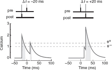
Figure 6.2 The synaptic model proposed by Graupner and Brunel (2012) reproduces STDP. The protocol for inducing long-term modifications is illustrated at the top (left for LTD, right for LTP). When the post-synaptic action potential precedes the pre-synaptic spike, the calcium variable c(t) (indicated with ‘calcium’ on the figure) spends more time between the two dashed lines than above the upper line (see the shaded areas of different gray levels below the curve), eventually inducing long-term depression (left). When the pre-synaptic spike precedes the post-synaptic action potential (right), the calcium variable is above the upper line for a significant fraction of time and it induces a long-term potentiation. Notice that the pre-synaptic spike induces a jump on the post-synaptic calcium concentration with a short delay, whereas the post-synaptic action potential has an instantaneous effect. Adapted from Graupner and Brunel (2012). Reproduced with permission of PNAS
6.3.2 Implementing a Synaptic Model in Neuromorphic Hardware
We now describe a typical procedure for designing a neuromorphic plastic synapse. We start from the theoretical model of the synaptic dynamics and we show how to transform it into a model in which the synapse is multistable (discrete) and hence implementable in hardware. This step requires the introduction of slow stochastic learning (see Section 6.2.3), and hence of a mechanism that transforms an inherently deterministic synapse which varies continuously into a stochastic synapse that is discrete on long timescales. In particular we show that spike-driven synapses can naturally implement stochastic transitions between the stable states, provided that the activity is sufficiently irregular.
We illustrate all these points with a paradigmatic example: we consider the case of auto-associative neural networks like the Hopfield model (Hopfield 1982), in which each memory is represented by a specific pattern of neural activity (typically a pattern of mean firing rates) that is imposed to the network at the time the pattern is memorized. The memory is recalled by reactivating the same or a similar pattern of activity at a later time, letting the network dynamics relax, and observing the stable, self-sustaining pattern of activity that is eventually reached. This pattern represents the stored memory, and it can be recalled by reactivating only a small fraction of the stored memory (pattern completion). In this simple example, the task is to implement an auto-associative content addressable memory; the type of learning we need is ‘supervised’ (in the sense that we know the desired neural output for each given input), the memories are represented by stable patterns of mean firing rates, and they are retrieved by reactivating a certain fraction of the initially activated neurons.
In order to design a synaptic circuit that implements this auto-associative memory, we need first to understand how the synapses should be modified when the patterns are memorized. In this case, the prescription has been found by Hopfield (1982), and it basically says that for each memory we need to add to the synaptic weight the product of the pre- and post-neural activities (under the simplifying assumption that the neurons are either active if they fire at high rate, or inactive if they fire at low rate, and the neural activity is represented by a +1 activity). The rule is basically a covariance rule and it is similar to the perceptron rule (see Section 6.4 for more details).
There are several similar prescriptions for different learning problems and they can be found in any textbook on neural network theory (see, e.g., Hertz et al. 1991 and Dayan and Abbott 2001 for examples of supervised, unsupervised, and reinforcement learning).
From Learning Prescriptions to Neuromorphic Hardware Implementations
Most of the learning prescriptions known in the neural network literature have been designed for simulated neural systems in which the synaptic weights are unbounded and/or continuous valued variables. As a consequence it is difficult to implement them in neuromorphic hardware. As we have seen in the previous section on memory retention, this is not a minor problem. In general, there is no standard procedure to go from the theoretical learning prescription to the neuromorphic circuit. We will describe one successful example which illustrates the typical steps that lead to the design of a synaptic circuit.
Consider again the problem of the auto-associative memory. If we denote by ξj the pre-synaptic neural activity, and by ξi the post-synaptic neural activity, then the Hopfield prescription says that every time we store a new memory we need to modify the synaptic weight wij as follows:
wij → wij + ξiξi,
where ξ = ±1 correspond to high and low firing rates (e.g., ξ = 1 corresponds to ν = 50 Hz and ξ = −1 corresponds to ν = 5 Hz). As we will show later in this chapter, it is possible to implement bistable synapses in neuromorphic hardware. In such a case wij has only two states, and every time we store a new memory we need to decide whether to modify the synapse and in which direction. As explained in the previous section on memory retention, bistable synapses can encode only one memory, unless the transitions between the two states occur stochastically. A simple rule that implements this idea is the following:
- Potentiation: wij → +1 with probability q if ξiξj = 1.
- Depression: wij → −1 with probability q if ξiξj = −1.
In all the other cases the synapse remains unchanged. This new learning prescription, proposed by Amit and Fusi (1992 1994) and Tsodyks (1990), implements an auto-associative memory and it behaves similarly to the Hopfield model. However, the memory capacity goes from p = αN to ![]() because of the limitations described in the previous section. How can we now translate this abstract rule into a real synaptic dynamics? This is described in Section 6.3.2.
because of the limitations described in the previous section. How can we now translate this abstract rule into a real synaptic dynamics? This is described in Section 6.3.2.
Spike-Driven Synaptic Dynamics
Once we have a learning prescription for a synapse that is implementable in hardware (e.g., a bistable synapse), we need to define the synaptic dynamics. The details of the dynamics will in general depend on how memories are encoded in the patterns of neural activity. In the case of the example of an auto-associative memory, the memories are assumed to be represented by patterns of mean firing rates. However, most of the hardware implementations are based on spiking neurons and hence we need to consider a synapse that can read out the spikes of pre- and post-synaptic neurons, estimate the mean firing rates, and then encode them in the synaptic weight.
Here we consider one model (Fusi et al. 2000) which is compatible with STDP, but it was designed to implement the rate-based auto-associative network described in Section 6.2 in neuromorphic hardware. Interestingly, noisy pulsed neural activity can naturally implement the stochastic selection mechanism described in the previous section, even when the synaptic dynamics are inherently deterministic. We illustrate the main ideas by presenting a simple paradigmatic example. The same principles are applied to most of the current hardware implementations.
Designing a Stochastic Spike-Driven Bistable Synapse
We consider now the scenario described in the previous section in which the relevant information about a memory is encoded in a pattern of neural firing rates. Each memory is represented by a pattern of activity in which, on average, half of the neurons fire at high rates and half of the neurons fire at low rates. Inspired by the cortical recordings in vivo, we assume that the neural activity is noisy. For example, the pre- and post-synaptic neurons emit spikes according to a Poisson process. If these stochastic processes are statistically independent, each synapse will behave in a different way, even if it experiences the same pre- and post-synaptic average activities. These processes can implement the simple learning rule described in the previous section, in which the synapses make a transition to a different stable state only with some probability q.
Indeed, consider a synapse which is bistable in the absence of spikes, that is, if its internal state variable X is above a threshold, then the synapse is attracted to the maximal value, otherwise it decays to the minimal value (see the mid plots in Figure 6.3). The maximum and the minimum are the only two stable synaptic values. The synaptic efficacy is strong if X is above the threshold and weak if X is below the threshold.
Every pre-synaptic spike (top plots) kicks X up and down depending on whether the post-synaptic depolarization (bottom plots) is above or below a certain threshold, respectively. When a synapse is exposed to stimulation, X can cross the threshold or remain on the same side where it was at the beginning of the stimulation. In the first case the synapse makes a transition to a different state (Figure 6.3, left), while in the second case, no transition occurs (Figure 6.3, right). Whether the transition occurs or not depends on the specific realization of the stochastic processes which control the pre- and the post-synaptic activities. In some cases there are enough closely spaced pre-synaptic spikes that coincide with elevated post-synaptic depolarization and the synapse can make a transition. In other cases the threshold is never crossed and the synapse returns to the initial value. The fraction of cases in which the synapse makes a transition determine the probability q which controls the learning rate. Notice that the synaptic dynamics are entirely deterministic and the load of generating stochasticity is transferred outside the synapse. Such a mechanism has been introduced in Fusi et al. (2000) and more recently has been applied to implement the stochastic perceptron (Brader et al. 2007; Fusi 2003). More details of the VLSI synaptic circuit can be found in Section 8.3.2 of Chapter 8. Interestingly, deterministic networks of randomly connected neurons can generate chaotic activity (van Vreeswijk and Sompolinsky 1998) and in particular the proper disorder which is needed to drive the stochastic selection mechanism (Chicca and Fusi 2001).
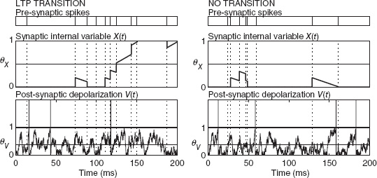
Figure 6.3 Spike-driven synaptic dynamics implementing stochastic selection. From top to bottom: pre-synaptic spikes, synaptic internal state, and post-synaptic depolarization as a function of time. Left: the synapse starts from the minimum (depressed state) but between 100 and 150 ms crosses the synaptic threshold θX and ends up in the potentiated state. A transition occurred. Right: the synapse starts from the depressed state, it fluctuates above it, but it never crosses the synaptic threshold, ending in the depressed state. No transition occurred. Notice that in both cases the average firing rates of the pre- and post-synaptic neurons are the same. Adapted from Amit and Fusi (1994). Reproduced with permission of MIT Press
The Importance of Integrators in Bistable Synapses
Spikes are events that are highly local in time, especially in the electronic implementations (they last 1 ms in biology, significantly less in most VLSI implementations). One of the main difficulties of dealing with these short events is related to the necessity of implementing a stochastic transition between synaptic states. In the relatively long intervals between two successive spikes, no explicit information about the activity of the pre- and post-synaptic neurons is available to the synapse. If the stochastic mechanism is implemented by reading out the instantaneous random fluctuations of the neural activity, then we need a device which constantly updates an estimate of the instantaneous neural activity. Any integrator can bridge the gap between two consecutive spikes or related events, and it can naturally measure quantities like the inter-spike intervals (e.g., in an RC circuit driven by the pre-synaptic spikes, the charge across the capacitor is an estimate of the instantaneous firing rate of the pre-synaptic neuron). The presence of an integrator seems to be a universal requirement for all hardware implementations of a synapse (electronic or biological). It is known that in biological synapses a few coincidences of pre- and post-synaptic spikes are needed to occur within a certain time interval to start the processes that lead to long-term modifications. Analogously, in all VLSI implementations, it seems to be necessary to accumulate enough ‘events’ before consolidating the synaptic modification. In the case of the described synapse, the events are the coincidences of pre-synaptic spikes and high post-synaptic depolarization (for LTP). In the case of pure STDP implementations (Arthur and Boahen 2006), they are the occurrence of pre- and post-synaptic spikes within a certain time window. In all these cases, an integrator (the variable X in the example) is not only important for implementing the stochastic transitions, but also protects the memory from the spontaneous activity, which otherwise would erase all previous synaptic modifications in a few minutes.
Spike-Driven Synaptic Models Implementing the Perceptron
The synaptic model described in Figure 6.3 can be extended to implement the perceptron algorithm described above. The dynamics already described essentially implement the synaptic modification expressed by
![]()
The perceptron algorithm is based on the same synaptic modifications, but it is complemented by the condition that the synapse should be updated only when the output neuron does not already respond as desired. In other words, the synapse should not be modified every time the total synaptic input Iμ is above the activation threshold and the desired output is active, that is, oμ = 1. An analogous situation occurs when the total synaptic input Iμ < θ and oμ = −1.
This condition can be implemented in synaptic dynamics as suggested in Brader et al. (2007). During training, the post-synaptic neuron receives two inputs, one from the plastic synapses, Iμ, and other from the teacher ![]() . The teacher input steers the activity of the output neuron toward the desired value. Hence it is strongly excitatory when the neuron should be active and weak or inhibitory when the neuron should be inactive (
. The teacher input steers the activity of the output neuron toward the desired value. Hence it is strongly excitatory when the neuron should be active and weak or inhibitory when the neuron should be inactive (![]() , where α is a constant, and oμ = ±1 depending on the desired output). After training, the plastic synapses should reach a state for which Iμ > θ when oμ = 1 and Iμ < θ when oμ = −1. These conditions should be verified for all input patterns μ = 1, …, p. Every time the desired output is achieved for an input pattern, the synapses should not be updated and the next input pattern should be considered. When these conditions are verified for all input patterns, then learning should stop.
, where α is a constant, and oμ = ±1 depending on the desired output). After training, the plastic synapses should reach a state for which Iμ > θ when oμ = 1 and Iμ < θ when oμ = −1. These conditions should be verified for all input patterns μ = 1, …, p. Every time the desired output is achieved for an input pattern, the synapses should not be updated and the next input pattern should be considered. When these conditions are verified for all input patterns, then learning should stop.
The main idea behind the implementation of the perceptron algorithm suggested in Brader et al. (2007) is that it is possible to detect the no-update condition by monitoring the activity of the post-synaptic neuron. Specifically, the synapses should not be updated every time the total synaptic input I + It is either very high or very low. Indeed, under these conditions, it is likely that I and It already match and that the neuron would respond as desired also in the absence of the teacher input: the maximum of the total synaptic input is reached when both I and It are large, and the minimum when both I and It are small. In both these cases the synapses should not be modified (e.g., when It is large it means that o = +1 and the synapses should not be modified whenever I > θ).
The mechanism is implemented by introducing an additional variable, called the calcium variable c(t), by Brader et al. (2007) for its analogies with the calcium concentration in the post-synaptic biological neuron. This variable integrates the post-synaptic spikes, and it represents an instantaneous estimate of the mean firing rate. When θc < c(t) < θp, then the synaptic efficacy is pushed toward the potentiated value whenever a pre-synaptic spike arrives and the post-synaptic depolarization is above a threshold Vθ, as in the synapse described in Figure 6.3. When θc < c(t) < θd, then the synaptic efficacy is depressed every time a pre-synaptic spike arrives and the post-synaptic depolarization is below Vθ.
Values of c(t) outside these ranges gate the synaptic modification and leave the synapse unchanged. The dynamics can be summarized by saying that for too large or too small values of the post-synaptic mean firing rate, the synapses are not modified. Otherwise they are modified according to the dynamics of Figure 6.3. The transitions between stable states remain stochastic, as in the simpler synaptic model, and the main source of stochasticity remains in the irregularity of the pre- and post-synaptic spike trains. The only difference is the gating operated by the calcium variable, which basically implements the perceptron condition of no-update whenever the output neuron responds correctly to the input.
6.4 Toward Associative Memories in Neuromorphic Hardware
We discussed in the previous sections how memories are stored and then retained in the pattern of synaptic states. We now discuss the process of memory retrieval, which unavoidably involves neural dynamics. Indeed, the synaptic states can be read out only by activating the pre-synaptic neuron and ‘observing’ the effects on the post-synaptic side. This is what is continuously done when the neural dynamics develop in response to a sensory input, or spontaneously, when driven by internal interactions. The repertoire of dynamic collective states that neural networks can express is rich (see Vogels et al. 2005 for a review of models of neural dynamics) and, depending on the experimental context of reference, the emphasis has been put on global oscillations (see Buzsaki 2006 for a recent overview), possibly including states of synchronous neural firing; chaotic states (see, e.g., Freeman 2003); stationary states of asynchronous firing (see, e.g., Amit and Brunel 1997; Renart et al. 2010). In what follows we will focus on a specific example in which memories are retrieved in the form of attractors of the neural dynamics (stable states of asynchronous firing). Many of the problems that we will discuss are encountered in the other memory retrieval problems.
6.4.1 Memory Retrieval in Attractor Neural Networks
Attractors can take many forms, such as limit cycles for oscillatory regimes, strange attractors for chaotic systems, or point attractors for systems endowed with a Lyapunov function. It is the latter point attractor case that will concern us in what follows. A point attractor for a neural network is a collective dynamic state in which neurons fire asynchronously with a stationary pattern of constant firing rates (up to fluctuations). If neurons are transiently excited by a stimulus, the network state relaxes to the nearest (in a sense to be made precise) attractor state (a point in the abstract network state space, whence the name).
The specific set of attractor states available to the network is dictated by the synaptic configuration. The idea of point attractors most naturally lends itself to the implementation of an associative memory, the attractor states being the memories that are retrieved given a hint in the form of an induced initial state of neural activities. In early models of associative memory the goal was to devise appropriate synaptic prescriptions ensuring that a prescribed set of patterns of neural activities were attractors of the dynamics.
Though suggestive of learning, this was much less, indeed a kind of existence proof for a dynamic scenario that experimental neuroscience strongly seemed to support (more on this later); the deep issue remained, of how to model the supervised, unsupervised or reinforce-based learning mechanisms driven by the interaction of the brain with its environment, and the generation of related expectation.
The Basic Attractor Network and the Hopfield Model
It is instructive to provide a few details on the working of such models of associative memory (of which the Hopfield model is of course the first successful example), as an easy context to grasp the key interplay between the dynamics of neural states and the structure of the synaptic matrix. In doing this, we will take a step back from the description level of the previous section; we will later consider attractor networks of spiking neurons.
First, in the original Hopfield model, neurons are binary, time-dependent variables. Two basic biological properties are retained in a very simple form: the neuron performs a spatial integration of its inputs, and its activity state can go from low to high if the integrated input exceeds a threshold. In formulae,
where N is the number of neurons in the (fully connected) network, wij is the efficacy of the synapse connecting pre-synaptic neuron j to the post-synaptic neuron i; the dynamics describe a deterministic change of neural state upon crossing the threshold θ.
The dynamics tend to ‘align’ the neural state with the ‘local field’:
The dynamics of the network can be described by introducing a quantity, the energy, that depends on the collective state of the network and that decreases at every update. If such a quantity exists, and this is always the case for symmetric synaptic matrices, then the network dynamics can be described as a descent toward the states with lower energy, eventually relaxing at the minima. In the case of the Hopfield model, the energy is
For the deterministic asynchronous dynamics, at each time step at most one neuron (say sk) changes its state, whereupon, writing

we get
so if sk does not change its state, ΔE(t) = 0; if it does, ΔE(t) < 0. If noise is added to the dynamics, the network does not settle into a fixed point corresponding to a minimum of E, but it will fluctuate in its proximity.
The key step was to devise a prescription for the {wij} such that pre-determined patterns are fixed points of the dynamics. This brings us to the seminal proposal by Hopfield (1982); to approach it let us consider first the case in which we choose just one pattern (one specific configuration of neural states) {ξi}, i = 1, …, N, with ξi = ±1 chosen at random, and we set the synaptic matrix as
![]()
Substituting into Eq. (6.4) we see that the configuration {si = ξi}, i = 1, …, N, is a minimum of E, which attains its smallest possible value, ![]() . The configuration is also easily verified to be a fixed point of the dynamics (Eq. 6.2), since
. The configuration is also easily verified to be a fixed point of the dynamics (Eq. 6.2), since
![]()
The network state {ξi} attracts the dynamics even if some (less than half) si ≠ ξi, which implements a simple instance of the key ‘error correction’ property of the attractor network: a stored pattern is retrieved from a partial initial information.
The celebrated Hopfield prescription for the synaptic matrix extends the above suggestion to multiple uncorrelated patterns ![]() independently for all i, μ):
independently for all i, μ):
Of course the question is whether the P patterns ![]() act simultaneously as attractors of the dynamics; as expected, this will depend on the ratio P/N. A simple argument based on a signal-to-noise analysis gives an idea of the relevant factors.
act simultaneously as attractors of the dynamics; as expected, this will depend on the ratio P/N. A simple argument based on a signal-to-noise analysis gives an idea of the relevant factors.
Analogously to the case of one pattern, one can ask about the stability of a given pattern ξν, for which the pattern has to be aligned with its local field ![]() :
:
The first term is a ‘signal’ component of order 1; the second term is zero mean ‘noise.’ It is the sum of ≃ NP uncorrelated terms of order 1, and that can be estimated to be of order ![]() . Therefore, the noise term is of order
. Therefore, the noise term is of order ![]() and is negligible as long as P ≪ N.
and is negligible as long as P ≪ N.
The prescription for wij can be transformed into a learning rule that is local in time by simply adding to the wij one pattern at the time. In other words, one can imagine a scenario in which a specific pattern of activity ξμ is imposed to the neurons. This pattern represents one of the memories that should be stored, and it induces the following synaptic modifications ![]() . When the procedure is iterated for all memories, we get the synaptic matrix prescribed by Hopfield. This form of online learning is what has been discussed in the previous section on memory storage.
. When the procedure is iterated for all memories, we get the synaptic matrix prescribed by Hopfield. This form of online learning is what has been discussed in the previous section on memory storage.
It should be noted that the prescription, Eq. (6.7), is by no means a unique solution to the problem; for example, choosing a matrix wij as a solution of ![]() would do for patterns that are linearly independent. However, this would be a nonlocal prescription, in that it would involve the inverse of the correlation matrix of the patterns ξ. The Hopfield prescription has the virtue of conforming to the general idea put forward by Hebb (1949) that a synapse connecting two neurons which are simultaneously active would get potentiated.
would do for patterns that are linearly independent. However, this would be a nonlocal prescription, in that it would involve the inverse of the correlation matrix of the patterns ξ. The Hopfield prescription has the virtue of conforming to the general idea put forward by Hebb (1949) that a synapse connecting two neurons which are simultaneously active would get potentiated.
In the retrieval phase, the network states in the Hopfield model populate a landscape with as many valleys as there are stored patterns (plus possibly the spurious ones mentioned above). The multiplicity of minima of E in the high-dimensional network state space suggests the celebrated landscape metaphor, a series of valleys and barriers separating them, in which the system evolves. In the deterministic case the representative point of the network state rolls down the closest valley floor from its initial condition, while noise can allow the system to cross barriers (with a typically exponential dependence of the crossing probabilities on the barrier height for given noise).
One valley is the ‘basin of attraction’ of the point attractor sitting at its floor: the set of initial states that lead ultimately to that attractor under the deterministic dynamics. Suggestive as it is, the usual one-dimensional landscape representation must be taken with caution, for the high dimensionality makes the intuitive grasp weaker; for example, the landscape gets populated with saddles, and the frontiers of the basins of attraction are high-dimensional themselves.
Attractors in Spiking Networks
In going from networks of binary neurons to networks of spiking neurons, most key features of the above picture are preserved, with some relevant differences. The workhorse in models of spiking neurons is the IF neuron: the membrane potential is a linear integrator with a threshold mechanism as a boundary condition on the membrane dynamics (see Chapter 7). The theory of diffusion stochastic processes provides the appropriate tools to analytically describe the IF neuron dynamics with noisy input (Burkitt 2006; Renart et al. 2004). The same formalism also provides the key to the description of a homogeneous recurrent population of IF neurons under the ‘mean field’ approximation: neurons in the population are assumed to share the same statistical properties (mean and variance) of the afferent currents; these are in turn determined by the average neurons’ firing rates and by the average recurrent synaptic efficacy. In an equilibrium state, any given neuron must generate spikes at an average rate which is the same as the other neurons’ one; this establishes a self-consistency condition that (at parity of other single-neuron parameters) determines the values of the average synaptic efficacy that allow for an equilibrium state. The mean field equations implementing such self-consistency condition equate the average firing rate to the single neuron response function, whose arguments (mean and variance of the input current) are now functions of the same average firing rate. For a typical, sigmoid-shaped response function, those equations posses either one stable solution (the firing rate of the only equilibrium state) or three solutions (fixed points), of which the two corresponding to the lowest and highest firing rates are stable.
In the latter case, if the spiking network sits in the lower fixed point and receives a sufficiently strong transient input, it can jump over the unstable state and, after the stimulus terminates, it will relax to the higher fixed point (see Figure 6.4).
The network can host multiple selective sub-populations, each of which is endowed with recurrent synapses that are strong with respect to the cross–sub-population ones. In a typical situation of interest, from a symmetric state of low activity, a stimulus selectively directed to a sub-population can activate an attractor state in which the transiently stimulated sub-population relaxes to a high-rate state, while the others are back to a low-rate state.
In a simulation, the sequence of events that lead to the activation of a selective attractor state would appear as in Figure 6.4. We remark that in the dynamic coupling between sub-populations that lead to the above scenario, a prominent role is played by the interplay between excitatory and inhibitory neurons.
Early examples proving the feasibility of such dynamic processes, generating attractor states in networks of spiking neurons with spike-driven synapses, were provided in simple settings by Del Giudice et al. (2003) and Amit and Mongillo (2003). More complex scenarios have been recently considered (Pannunzi et al. 2012). This study aims at modeling experimental findings from recordings during a visual classification task: a differential modulation of neural activity is observed for visual features defined as relevant or irrelevant for the classification task. Under the assumption that such modulation would emerge due to a selective feedback signal from areas implementing the categorical decision, a multimodular model was set up, with mutual interactions between feature-selective populations and decision-coding ones. It was possible to demonstrate learning histories bringing the initially unstructured network to a complex synaptic structure supporting successful performance on the task and also the observed task-dependent modulation of activity in the IT populations.

Figure 6.4 Activation of persistent delay activity, selective for a familiar stimulus, in a simulation of synaptically coupled spiking neurons. Potentiated synapses connect excitatory neurons encoding the same stimulus. The raster plot (a) shows the spikes emitted by a subset of cells in the simulated network, grouped in sub-populations with homogeneous functional and structural properties. The bottom five raster strips refer to neurons selective to five uncorrelated stimuli; the raster in the upper strip refers to a subset of inhibitory neurons, and the large middle strip to background excitatory neurons. (b) The emission rates of the selective sub-populations are plotted (the fraction of neurons emitting a spike per unit time). The population activity is such that before the stimulation all the excitatory neurons emit spikes at low rate (global spontaneous activity) almost independently of the functional group they belong to. When one of the selective sub-populations is stimulated (for the time interval indicated by the gray vertical strips), upon releasing the stimulation, that sub-population relaxes to a self-sustaining state of elevated firing activity, an expression of attractor dynamics. Adapted from Del Giudice et al. (2003), Copyright 2003, with permission from Elsevier
6.4.2 Issues
The Complex Interactions Between Neural and Synaptic Dynamics
In attractor models based on a prescription for the synaptic matrix, the implicit assumption is that the synaptic matrix can be made to emerge through some forms of biologically plausible learning mechanisms. This, however, conceals several subtleties and pitfalls. In fact, it is perhaps surprising that to date few efforts have been devoted to studying how attractor states can dynamically emerge in a neural population as the result of the ongoing neural spiking activity, determined by the flow of external stimuli and the feedback in the population, and biologically relevant spike-driven synaptic changes (Amit and Mongillo 2003; Del Giudice et al. 2003; Pannunzi et al. 2012).
We now consider the familiar scenario of attractor states as memory states in an associative memory, though most remarks have more general validity. A very basic observation is that in a recurrent network the neural and synaptic dynamics are coupled in a very intricate way: synaptic modifications are (slowly) driven by neural activities, which are in turn determined by the pattern of synaptic connections at any given time. An incoming stimulus will both provoke the relaxation of the network to an attractor state, selective for that stimulus (if an appropriate synaptic structure exists at that point), and will also promote synaptic changes depending on the spiking activity it imposes on the network; learning and retrieval are now intertwined processes.
Even well before facing problems of memory capacity, the stability of the relevant neural states are challenged by the above dynamic loop between neural and synaptic dynamics. In fact, once the neural activities repeatedly evoked by a stimulus have left a trace in the synaptic matrix, sufficient to support a selective persistent attractor state, the following spectrum of neural activities emerge: a ‘spontaneous’ state of low firing activity (νspon); a state of high firing corresponding to the response to the external stimulus (νstim); the state of intermediate and selective firing activity, supported by feedback, which persists after the stimulus is gone in the absence of large perturbations (νsel).
A natural request is that in the absence of incoming stimuli, the structured network should be able to keep its memory stable for long times; if spontaneous activity could modify the synapses, or the synaptic matrix could significantly change in the attractor state, any memory state would be doomed to fade away, or the last one to be evoked would dramatically interfere with other memories embedded in the same synaptic matrix at that stage (if the attractor state is left undisturbed for long and the representations of different memories overlap). Hence it is important that the synaptic dynamics is designed so that synaptic changes occur only during stimulation, driven by spikes at average rate νstim (see Section 6.3 on memory storage). But as the synapses go on changing, so do both νstim and νsel, in general by different amounts, and in order for the above constraint to be met all along the learning process, we must have, comparing early and late stages of learning, ![]() .
.
In the regime of slow learning that is of interest, a ‘good’ learning trajectory of the network (i.e., the sequence of synaptic configurations traveled by the network on its way to the onset of selective attractor states) should be a sequence of quasi-equilibrium states. These sequences would have the additional feature that can be studied and controlled by mean field theory approximations. Finally, the parameters of the synaptic model must be tuned to guarantee a balance between LTD and LTP at each learning stage. The introduction of a suitable regulatory mechanism would probably relax this strict requirement.
Finite-Size Effects
Any real network has a finite number of neurons N. Finite-size effects are important and bring about deviations from the predictions of the mean field theory. In particular, for finite N each population has a distribution of emission rates. Let us consider the synapses connecting populations of neurons stimulated by the same stimulus, and therefore supposed to get potentiated: the high- and low-rate tails of the actual frequency distribution corrupt the homogeneity of the pattern of synaptic transition probabilities, such that in the same synaptic group some synapses will have too high LTP probability, while others will be unexpectedly unchanged. Similarly, finite-size effects can provoke unwanted synaptic transitions where they are not expected and harmful (such as a potentiation of synapses involving post-synaptic background neurons, which can become the seed of instability for the spontaneous state).
One ingredient which makes finite-size effects more or less harmful is the character of the ‘synaptic transfer function’, that is the function giving the LTP/LTD transition probabilities as functions of the pre- and post-synaptic emission rates. The sensitivity of this function in the critical region where the rate distributions involved overlap is an important factor in determining how serious finite-size effects are going to be.
6.5 Attractor States in a Neuromorphic Chip
In a way that cannot be articulated in the present context, point attractors can be viewed as the basic, discrete ‘symbols’ of complex and dynamic ‘words’ that constitute the brain’s inner dialog. This is, at best, the identification of the elements for the definition of a computational paradigm, the latter being still far from reach. However, the recognition of the potential computational role of attractors is a good motivation to embody attractor dynamics in neuromorphic VLSI chips, which after all purport ultimately to compute as the brain does.
We sketch here some recent results obtained in the attempt to establish and control attractor dynamics in neuromorphic chips of spiking neurons. We give in sequence an example of memory retrieval (i.e., the activation of a pattern of firing rates which is correlated with a previously embedded synaptic structure), and a simple example in which an attractor representation is dynamically constructed in the VLSI network, from the repeated presentation of visual stimuli acquired by a neuromorphic sensor in real time.
6.5.1 Memory Retrieval
We first summarize recent work which, for the first time, demonstrates robust working memory states based on attractor dynamics in a bistable spiking neural network implemented with neuromorphic VLSI hardware (Giulioni et al. 2011). The on-chip network (see Figure 6.5) consists of three interacting populations (two excitatory, one inhibitory) of leaky integrate-and-fire (LIF) neurons. One excitatory population (the Eatt population in the network of Figure 6.5) has strong synaptic self-excitation, which selectively sustains meta-stable states of ‘high’- and ‘low’-firing activity (the remaining excitatory neurons compose an unselective background). Depending on the overall excitability, transitions of Eatt activity from the ‘low’ to the ‘high’ state may be evoked by a transient external stimulation (with reference to Figure 6.5, a temporary increase in the external mean firing rate of E1AER and/or IAER); the ‘high’ state retains a ‘working memory’ of a stimulus until well after its release. In a small network such as the one implemented in the chip, state switches can also occur spontaneously due to random activity fluctuations; such cases are interesting but will not be examined here.
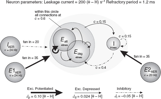
Figure 6.5 Architecture of the network implemented on a VLSI chip with 128 neurons and 16,384 plastic reconfigurable synapses, designed after the model described in Section 6.3.2. Besides the populations Eatt, Ebkg, and I of excitatory and inhibitory neurons, physically residing in the chip, input to the network is provided by further populations emulated on a PC, whose activity is forwarded in real time by a suitable AER communication infrastructure. Adapted from Giulioni et al. (2011). Reproduced with permission of the authors
The effect of excitatory and inhibitory input transients to Eatt is illustrated in Figure 6.6. The average firing of Eatt and Ebkg neurons is shown during four successive stimuli, two excitatory and two inhibitory. The first excitatory stimulus is weak; the network reacts in a quasi-linear regime, with a slight activity increase of Eatt. After the stimulus is released Eatt returns to the ‘low’ meta-stable state.
The second, stronger excitatory stimulus causes a nonlinear response in the strongly self-coupled Eatt population and dramatically increases its activity (to a lesser degree Ebkg activity is also affected). The recurrent interactions of the network (far more than the external stimulus itself) drive the network to a ‘high’ state. After the stimulus is removed the network relaxes to its ‘high’ meta-stable state thereby preserving a ‘working memory’ of the earlier stimulus.

Figure 6.6 Firing rates of Eatt and Ebkg in response to multiple input transients. Excitatory (inhibitory) transients are created by square-pulse increments of E1AER (IAER) activity. The timing of input transients is illustrated beneath the main panel: 0.5 and 1.5 s mark the onset of subthreshold (νE1 = 34 Hz) and supra-threshold (νE1 = 67, 84, or 115 Hz) excitatory ‘kicks’, 3 and 4 s that of sub- and supra-threshold inhibitory ‘kicks.’ Subthreshold ‘kicks’ merely modulate activity of the current meta-stable state. Supra-threshold ‘kicks’ additionally trigger a transition to the other meta-stable state. Adapted from Giulioni et al. (2011). Reproduced with permission of the authors
In a similar manner, inhibitory stimuli can induce a return transition to the ‘low’ meta-stable state. In Figure 6.6, a weak inhibitory stimulus was applied at t = 3 s and a strong inhibitory one at t = 4 s. The former merely shifted temporarily the ‘high’ state, to which Eatt is attracted back after the end of the stimulus, thus leaving the ‘working memory’ state intact. The latter was sufficiently hefty to destabilize the ‘high’ state, thus forcing the system to return to the ‘low’ state.
The ‘working memory’ state is therefore robust against activity fluctuations and small perturbations, a manifestation of the attractor property.
6.5.2 Learning Visual Stimuli in Real Time
While it is interesting to show that the VLSI network is able to exhibit robust attractor dynamics for a suitable preset synaptic structure, it is by no means obvious that such synaptic structure can be autonomously generated by the dynamic coupling between the ongoing, stimulus-induced neural activity and the consequent changes in the plastic synapses, which in turn affects the neural response to stimuli (see the discussion in Section 6.4.2). As already noted, this is difficult to achieve for theoretical models, let alone for neuromorphic chips. In this section we demonstrate the learning ability of our on-chip network in a simple, but nontrivial, example (a very preliminary account has been given in Giulioni and Del Giudice 2011). The network architecture is similar to the one depicted in Figure 6.5, but here we use a total of 196 excitatory neurons and 50 inhibitory ones. The network is distributed over two identical chips hosted in the setup shown in Figure 6.7, the inter-chip connectivity being defined by a writable look-up-table in the PCI-AER board. External stimuli come from the dynamic vision sensor retina (Lichtsteiner et al. 2008) which encodes in patterns of AER spikes variations of light intensity in its visual fields. Spikes emitted by the retina are routed toward the chips through the PCI-AER board. The entire system runs in real time and both neural activities and synaptic states are monitored (again through the PCI-AER board). Plastic synapses between excitatory neurons are designed after the model introduced in Fusi et al. (2000) and discussed above.
The visual field of the retina is divided in 196 macropixels, each corresponding to a square of 9 × 9 retina pixels, and each macropixel is the input source to a single neuron in the on-chip network. From this mapping it is possible to visualize the network firing rates to match the geometric arrangement of the macropixels (see the matrices in Figure 6.8). All synapses are set to be depressed at the beginning of the experiment; given a chosen stimulus structure, learning is expected to selectively potentiate synapses connecting neurons which are co-active for that stimulus. Three visual stimuli were chosen for the experiment illustrated in Figure 6.8, each activating about one-fourth of the neurons in the network (one-fourth of the neurons constitute a background, unselective population). Since the retina is sensitive only to temporal variations of luminosity contrast, a stimulus is presented to the retina as a patterns of black dots flickering on a white background. The portion of visual field not occupied by the stimulus is filled with a sparse noisy background eliciting low activity in the silicon retina.
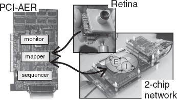
Figure 6.7 Hardware setup for the learning experiments. A PCI-AER board implements the mapping between the neuromorphic retina and the neurons in the recurrent network, in terms of macro-pixels, and manages the asynchronous communication between the retina and the network, which is distributed on two chips. Adapted from Giulioni and Del Giudice (2011). Reproduced with permission of the authors

Figure 6.8 Top panel: input visual stimuli shown on the screen (on the left for each pair) and their reconstruction from the network activity after the learning period. Input stimuli are active per 0.4 s per trial. Data for the image reconstruction are recorded during the working memory phase, after the stimulus removal. Each macropixel corresponds to a neuron in the network. Gray levels encode for neurons’ firing rates. Central panel: mean firing rates of the three neuronal groups activated by the three (orthogonal) input stimuli. Lower panel: fraction of potentiated synapses, read before every learning trial. Each line reports the time course of the fraction of potentiated recurrent synapses, among those connecting neurons encoding the same input stimulus. Above about 70% potentiation we observe self-sustaining, working memory states in the neural activity. All the synapses connecting neurons encoding different stimuli, and neuron encoding stimuli to background neurons, remain depressed throughout the entire experiment (not shown)
The learning protocol consists of repetitive presentations of the visual stimuli to the retina, as illustrated in Figure 6.8. In the same figure we also report the network response and the evolution of the synapses during learning.
In the absence of visual stimulation, the initial network is in a low-activity state. In the early stages of learning, when the stimulus is removed, the network goes back to this low-activity state.
After repeated presentations, a selective synaptic structure builds up, such that the mature network is able, after the removal of the stimulus, to sustain a noisy but recognizable representation of the learned visual pattern. From Figure 6.8 it is seen that for the mature network (t > 120 s) the stimulus elicits a fast response of the selective excitatory sub-population; after stimulus removal the selective activity is kept elevated (because of the strong self-excitation generated by learning). After the high state persists for more than about 2 s, it decays spontaneously back to the low state; indeed, finite-size fluctuations are large in such small systems, and they affect the stability of attractor states in an important way. We stress that, in the chip, inhomogeneities and mismatch cause a wide dispersion of effective synaptic parameters, in the face of which we obtain robust learning histories.
We also confirmed (not shown) that the mature network exhibits the expected pattern completion ability: upon presenting a degraded versions of a learned stimulus, the network is able to retrieve the activity pattern corresponding to the complete stimulus; learning is also robust with respect to the choice of the initial condition for the synaptic matrix.
6.6 Discussion
The theory covered by this chapter shows that there is a fundamental problem of scalability in neuromorphic devices with memory and online learning. The problem, related to the boundedness of the variables that represent the synaptic weights, is important as learning neuromorphic chips are mostly occupied by plastic synapses. Unfortunately the problem is only partially solved, with the consequence that current neuromorphic devices suffer from major limitations in their memory capacity. In the most efficient models that are available, the number p of storable dense memories scales with the square root of the number N of synapses, which is sufficient for performing a variety of different and interesting tasks, but it is far from what is achievable in neural networks with off-line learning, where p can scale linearly with N. In large-scale neural systems, which are now becoming implementable and further described in Chapter 16, neuromorphic devices with online learning are greatly disadvantaged in terms of memory capacity.
Some of the limitations of neuromorphic systems derive from the simplicity of the switch-like mechanisms used to implement plastic synapses. Not only does this simplicity contrast with the complexity of biological synapses, it also makes large-scale neuromorphic devices highly inefficient. Properly designed complex synapses can greatly increase the amount of information stored per memory (Fusi et al. 2005) and the number of storable memories (Benna and Fusi 2013), closing the gap between neural systems with online and off-line learning. However, these types of synapses are difficult to implement in hardware, and silicon area occupied by complex plastic synapses can be so large that it might be more efficient to use a larger number of simple synapses. It is unclear whether silicon synapses can actually benefit from complexity as much as their biological counterparts.
An alternative approach is to utilize simple bistable synapses in more structured memory systems. Memories can be distributed across multiple brain regions, each one characterized by a limited memory capacity (see, e.g., Roxin and Fusi 2013). This strategy can lead to improved memory performance, however it usually requires a complex neural machinery to transfer and organize information. More theoretical studies will be needed to determine the optimal implementation strategies for large-scale neural systems and most likely every problem will have a different solution.
A final challenge is to deal with heterogeneities (mismatch in electrical circuits). Biological systems can tolerate large variations in the parameters that characterize the dynamics of their elements. They may even take advantage of the diversity of their components. Neuromorphic analog devices have also to deal with heterogeneities which are not under control in the design of the chip. At the moment the electronic mismatch can be highly disruptive and it greatly limits the performance of neuromorphic devices. It is not inconceivable that in the future the diversity generated by mismatch will actually be harnessed to perform computation. This will require new theoretical studies for understanding the computational role of heterogeneity (see, e.g., Shamir and Sompolinsky 2006).
Whatever the form is of future models of plastic synapses which are amenable to microelectronic implementation, it will also determine constraints on the relevant theoretical description of the ensuing neural dynamics and its impact on our ability to control neuromorphic chips. We gave in Section 6.4 of this Chapter an example of the way mean field theory can be used as a conceptual guide to build a procedure for a model-driven ‘system identification’ approach to find relevant regions in the chip’s parameter space. The case shown, however, was still simple in that the system comprised few homogeneous populations. On the other hand, a theoretical compass to navigate the parameter space will be even more needed for neural systems with complex structured synaptic connectivity, unless the synaptic and neural elements will be endowed with self-tuning mechanisms, which will require additional complexity. The control of these new neural systems will probably require a new theory which will be able to deal with complex and highly heterogeneous neural networks.
References
Amit D. 1989. Modeling Brain Function. Cambridge University Press.
Amit DJ and Brunel N. 1997. Model of global spontaneous activity and local structured activity during delay periods in the cerebral cortex. Cereb. Cortex 7(3), 237–252.
Amit DJ and Fusi S. 1992. Constraints on learning in dynamic synapses. Netw.: Comput. Neural Syst. 3(4), 443–464.
Amit DJ and Fusi S. 1994. Learning in neural networks with material synapses. Neural Comput. 6(5), 957–982.
Amit DJ and Mongillo G. 2003. Spike-driven synaptic dynamics generating working memory states. Neural Comput. 15(3), 565–596.
Anthony M and Bartlett PL. 1999. Neural Network Learning: Theoretical Foundations. Cambridge University Press.
Arthur JV and Boahen K. 2006. Learning in silicon: timing is everything. In: Advances in Neural Information Processing Systems 18 (NIPS) (eds Weiss Y, Schölkopf B, and Platt J). MIT Press Cambridge, MA. pp. 75–82.
Babadi B and Abbott LF. 2010. Intrinsic stability of temporally shifted spike-timing dependent plasticity. PLoS Comput. Biol. 6(11), e1000961.
Ben Dayan Rubin DD, and Fusi S. 2007. Long memory lifetimes require complex synapses and limited sparseness. Front. Comput. Neurosci. 1(7), 1–14.
Benna M and Fusi S. 2013. Long term memory … now longer than ever. Cosyne 2013 II-1, 102–103.
Bi GQ and Poo MM. 1998. Synaptic modifications in cultured hippocampal neurons: dependence on spike timing, synaptic strength, and postsynaptic cell type. J. Neurosci. 18(24), 10464–10472.
Block HD. 1962. The perceptron: a model for brain functioning. I. Rev. Mod. Phys. 34(1), 123–135.
Brader JM, Senn W, and Fusi S. 2007. Learning real-world stimuli in a neural network with spike-driven synaptic dynamics. Neural Comput. 19(11), 2881–2912.
Burkitt A. 2006. A review of the integrate-and-fire neuron model: I. Homogeneous synaptic input. Biol. Cybern. 95(1), 1–19.
Buzsaki G. 2006. Rhythms of the Brain. Oxford University Press.
Chicca E and Fusi S. 2001. Stochastic synaptic plasticity in deterministic aVLSI networks of spiking neurons. In: Proceedings of the World Congress on Neuroinformatics (ed. Rattay F). ARGESIM/ASIM Verlag, Vienna. pp. 468–477.
Dayan P and Abbott LF. 2001. Theoretical Neuroscience. MIT Press.
Del Giudice P, Fusi S, and Mattia M. 2003. Modelling the formation of working memory with networks of integrate-and-fire neurons connected by plastic synapses. J. Physiol. Paris 97(4–6), 659–681.
Freeman WJ. 2003. Evidence from human scalp EEG of global chaotic itinerancy. Chaos 13(3), 1067–1077.
Fusi S. 2002. Hebbian spike-driven synaptic plasticity for learning patterns of mean firing rates. Biol. Cybern. 87(5-6), 459–470.
Fusi S. 2003. Spike-driven synaptic plasticity for learning correlated patterns of mean firing rates. Rev. Neurosci. 14(1–2), 73–84.
Fusi S and Abbott LF. 2007. Limits on the memory storage capacity of bounded synapses. Nat. Neurosci. 10(4), 485–493.
Fusi S and Senn W. 2006. Eluding oblivion with smart stochastic selection of synaptic updates. Chaos 16(2), 026112.
Fusi S, Annunziato M, Badoni D, Salamon A, and Amit DJ. 2000. Spike-driven synaptic plasticity: theory, simulation, VLSI implementation. Neural Comput. 12(10), 2227–2258.
Fusi S, Drew PJ, and Abbott LF. 2005. Cascade models of synaptically stored memories. Neuron 45(4), 599–611.
Gerstner W, Kempter R, van Hemmen JL, and Wagner H. 1996. A neuronal learning rule for sub-millisecond temporal coding. Nature 383(6595), 76–81.
Giulioni M and Del Giudice P. 2011. A distributed VLSI attractor network learning visual stimuli in real time and performing perceptual decisions. In: Frontiers in Artificial Intelligence and Applications – Proceedings of WIRN 2011 (eds Apolloni B, Bassis S, Esposito A, and Morabito CF). vol. 234. IOS press. pp. 344–352.
Giulioni M, Camilleri P, Mattia M, Dante V, Braun J, and Del Giudice P. 2011. Robust working memory in an asynchronously spiking neural network realized with neuromorphic VLSI. Front. Neuromorphic Eng. 5, 149.
Graupner M and Brunel N. 2012. Calcium-based synaptic plasticity model explains sensitivity of synaptic changes to spike pattern, rate, and dendritic location. Proc. Natl. Acad. Sci. USA 109(10), 3991–3996.
Gütig R and Sompolinsky H. 2006. The tempotron: a neuron that learns spike timing-based decisions. Nat. Neurosci. 9(3), 420–428.
Hebb DO. 1949. The Organization of Behavior: A Neuropsychological Theory. Wiley, New York.
Hertz J, Krogh A, and Palmer RG. 1991. Introduction to the Theory of Neural Computation. Addison Wesley.
Hinton G and Sejnowski TJ. 1999. Unsupervised Learning: Foundations of Neural Computation. MIT Press, Cambridge, MA.
Hopfield JJ. 1982. Neural networks and physical systems with emergent selective computational abilities. Proc. Natl. Acad. Sci. USA 79(8), 2554–2558.
Legenstein R, Naeger C, and Maass W. 2005. What can a neuron learn with spike-timing-dependent plasticity? Neural Comput. 17(11), 2337–2382.
Levy WB and Steward O. 1983. Temporal contiguity requirements for long-term associative potentiation/depression in the hippocampus. Neuroscience 8(4), 791–797.
Lichtsteiner P, Posch C, and Delbrück T. 2008. A 128 × 128 120 dB 15 us latency asynchronous temporal contrast vision sensor. IEEE J. Solid-State Circuits 43(2), 566–576.
Markram H, Lubke J, Frotscher M, and Sakmann B. 1997. Regulation of synaptic efficacy by coincidence of postsynaptic APs and EPSPs. Science 275(5297), 213–215.
Minsky ML and Papert SA. 1969. Perceptrons. MIT Press, Cambridge. Expanded edition 1988.
Nägerl UV, Köstinger G, Anderson JC, Martin KAC, and Bonhoeffer T. 2007. Protracted synaptogenesis after activity-dependent spinogenesis in hippocampal neuron. J. Neurosci. 27(30), 8149–8156.
O’Connor DH, Wittenberg GM, and Wang SSH. 2005. Graded bidirectional synaptic plasticity is composed of switch-like unitary events. Proc. Natl. Acad. Sci. USA 102(27), 9679–9684.
Pannunzi M, Gigante G, Mattia M, Deco G, Fusi S, and Del Giudice P. 2012. Learning selective top-down control enhances performance in a visual categorization task. J. Neurophys. 108(11), 3124–3137.
Parisi G. 1986. A memory which forgets. J. Phys. A. 19, L617.
Petersen CCH, Malenka RC, Nicoll RA, and Hopfield JJ. 1998. All-or-none potentiation at CA3-CA1 synapses. Proc. Natl. Acad. Sci. USA 95(8), 4732–4737.
Renart A, Brunel N, and Wang X. 2004. Mean-field theory of irregularly spiking neuronal populations and working memory in recurrent cortical networks. In: Computational Neuroscience: A Comprehensive Approach (eds Maass W and Bishop CM). Chapman and Hall/CRC. pp. 431–490.
Renart A, de la Rocha J, Bartho P, Hollender L, Parga N, Reyes A, and Harris KD. 2010. The asynchronous state in cortical circuits. Science 327(5965), 587–590.
Rosenblatt F. 1958. The perceptron: a probabilistic model for information storage and organization in the brain. Psychol. Rev. 65(6), 386–408. Reprinted in: Neurocomputing: Foundations of Research (eds Anderson JA and Rosenfeld E).
Rosenblatt F. 1962. Principles of Neurodynamics. Spartan Books, New York.
Roxin A and Fusi S. 2013. Efficient partitioning of memory systems and its importance for memory consolidation. PLoS Comput. Biol. 9(7), e1003146.
Sejnowski TJ. 1977. Storing covariance with nonlinearly interacting neurons. J. Math. Biol. 4, 303–321.
Senn W and Fusi S. 2005a. Convergence of stochastic learning in perceptrons with binary synapses. Phys. Rev. E. Stat Nonlin. Soft Matter Phys. 71(6 Pt 1), 061907.
Senn W and Fusi S. 2005b. Learning only when necessary: better memories of correlated patterns in networks with bounded synapses. Neural Comput. 17(10), 2106–2138.
Shamir M and Sompolinsky H. 2006. Implications of neuronal diversity on population coding. Neural Comput. 18(8), 1951–1986.
Shouval HZ, Wang SS, and Wittenberg GM. 2010. Spike timing dependent plasticity: a consequence of more fundamental learning rules. Front. Comput. Neurosci. 4(19), 1–13.
Sjöström PJ, Turrigiano GG, and Nelson SB. 2001. Rate, timing, and cooperativity jointly determine cortical synaptic plasticity. Neuron 32(6), 1149–1164.
Sompolinsky H. 1986. Neural networks with non-linear synapses and static noise. Phys. Rev. A 34, 2571.
Song S and Abbott LF. 2001. Cortical development and remapping through spike timing-dependent plasticity. Neuron 32(2), 339–350.
Song S, Miller KD, and Abbott LF. 2000. Competitive Hebbian learning through spike-timing-dependent synaptic plasticity. Nat. Neurosci. 3(9), 919–926.
Sutton RS and Barto AG. 1998. Reinforcement Learning: An Introduction. MIT Press.
Tsodyks M. 1990. Associative memory in neural networks with binary synapses. Mod. Phys. Lett. B4, 713–716.
van Vreeswijk C and Sompolinsky H. 1998. Chaotic balanced state in a model of cortical circuits. Neural Comput. 10(6), 1321–1371.
Vogels TP, Rajan K, and Abbott LF. 2005. Neural network dynamics. Annu. Rev. Neurosci. 28(1), 357–376.
__________
Two-photon microscopy images of a calcein-filled CA1 pyramidal neuron showing newly growing spines. Adapted from Figure 1 of Nägerl et al. (2007). Reproduced with permission of the Society for Neuroscience.