Chapter 2
Introduction to database server components
One of the best ways to develop a better understanding of SQL Server is to understand the infrastructure that supports the database. Having a better grasp of hardware, networking, availability options, security, and virtualization enables you to design, implement, and provision solutions that benefit your organization. Learning these concepts enables you to make good decisions to help create a stable environment for your databases. These decisions can affect anything from performance to uptime.
SQL Server runs on Windows and Linux, as well as in Linux containers. Microsoft has crafted the Database Engine to work the same way on other platforms as it does on Windows. The saying “it’s just SQL Server” applies, but here we highlight places where there are differences.
We first discuss hardware. No matter which configuration you end up using, there are four basic components in a database infrastructure:
Memory
Processor
Permanent storage
Network
We then introduce high availability (HA) offerings, including new functionality for availability groups introduced in SQL Server 2022. When considering strategies for SQL Server HA and disaster recovery (DR), you design according to the organization’s requirements for business continuity in terms of a Recovery Point Objective (RPO) and Recovery Time Objective (RTO).
We next provide an overview of security, including Active Directory, service principal names, federation and claims, and Kerberos. We cover ways to access the Database Engine, either on-premises or in Azure. As data theft has become more prevalent, you need to consider the security of the database itself, the underlying OS and hardware (physical or virtual), the network, and database backups.
Finally, we look at the similarities and differences between virtual machines (VMs) and containers, and when you should use them. Whether running on physical or virtual hardware, databases perform better when as much of the data as possible can be cached in memory and backed by fast, persistent storage that is redundant, with low latency and high random input/output operations per second (IOPS).
Memory
SQL Server is designed to use as much memory as it needs, and as much as you give it. By default, the upper limit of memory that SQL Server can access is limited only by the physical random-access memory (RAM) available to the server or to the edition of SQL Server you’re running (whichever is lower). SQL Server on Linux has additional memory limits to avoid out-of-memory (OOM) errors.
Understand the working set
The physical memory made available to SQL Server by the operating system (OS) is called the working set. This working set is broken up into several sections by the SQL Server Memory Manager. The two largest and most important sections are the buffer pool and the procedure cache, also known as the plan cache.
In the strictest sense, working set applies only to physical memory. However, as you will soon see, the buffer pool extension blurs the lines because it uses non-volatile storage.
We look deeper into default memory settings in Chapter 3, “Design and implement an on-premises database infrastructure,” in the “Configuration settings” section.
Cache data in the buffer pool
For best performance, SQL Server caches data in memory, because it is orders of magnitude faster to access data directly from memory than from traditional storage.
The buffer pool is an in-memory cache of 8 KB data pages that are copies of pages in the database file. Initially, the copy in the buffer pool is identical. Any changes to data are first applied to this buffer pool copy (and the transaction log) and then asynchronously applied to the data file.
When you run a query, the Database Engine requests the data page it needs from the buffer manager. (See Figure 2-1.) If the data is not already in the buffer pool, a page fault occurs. (This is an OS feature that informs the application that the page isn’t in memory.) The buffer manager fetches the data from the storage subsystem and writes it to the buffer pool. When the data is in the buffer pool, the query continues.

Figure 2-1 The buffer pool and the buffer pool extension.
The buffer pool is usually the largest consumer of the working set because it’s where your data is. If the amount of data requested for a query exceeds the capacity of the buffer pool, the data pages spill to a drive, using either the buffer pool extension or a portion of tempdb.
The buffer pool extension uses non-volatile storage to extend the size of the buffer pool. It effectively increases the database working set, forming a bridge between the storage layer where the data files are located and the buffer pool in physical memory.
For performance reasons, this non-volatile storage should be solid-state storage, directly attached to the server.
 To learn how to turn on the buffer pool extension, read the section “Configuration settings” in Chapter 3. To learn more about tempdb, read the section “Data files and filegroups,” also in Chapter 3.
Cached plans in the procedure cache
The procedure cache is usually smaller than the buffer pool. When you run a query, Query Optimizer compiles a query plan to explain to the Database Engine exactly how to run the query. To save time, it keeps a copy of that query plan so it won’t need to compile the plan each time the query runs. It is not quite as simple as this, of course—plans can be removed, and trivial plans are not cached, for instance—but it’s enough to give you a basic understanding.
The procedure cache is split into various cache stores by the Memory Manager. This is also where you can see if there are single-use query plans that are consuming memory.
- For more information about cached execution plans, read Chapter 14, “Performance tune SQL Server” or visit https://blogs.msdn.microsoft.com/blogdoezequiel/2014/07/30/too-many-single-use-plans-now-what/.
Lock pages in memory
When you turn on the lock pages in memory (LPIM) policy, Windows cannot trim (reduce) SQL Server’s working set.
Locking pages in memory ensures that Windows memory pressure cannot take resources away from SQL Server or push SQL Server memory into the Windows Server system page file, which dramatically reduces performance.
Under normal circumstances, Windows doesn’t “steal” memory from SQL Server flippantly; it is done in response to memory pressure on the Windows Server. Indeed, all applications can have their memory affected by pressure from Windows.
However, without the ability to relieve pressure from other applications’ or a virtual host’s memory demands, LPIM can prevent Windows from deploying enough memory to remain stable. Because of this, LPIM cannot be the only method used to protect SQL Server’s memory allocation.
Note
The Linux kernel is far stricter with memory management and forcibly terminates processes that use too much memory. With SQL Server on Linux, a dedicated setting called memory.memorylimitmb limits the amount of physical memory SQL Server can see. (By default, this is 80 percent of physical memory.) Chapter 5, “Install and configure SQL Server on Linux,” covers this in more detail.
The controversy of the topic is stability versus performance, in which the latter was especially apparent on systems with limited memory resources and older operating systems. On larger servers with operating systems since Windows Server 2008, there is a lesser need for this policy to insulate SQL Server from memory pressure.
The prevailing wisdom is that the LPIM policy should be turned off by default for SQL Server unless all the following conditions apply:
The server is virtual. See “Avoid overcommitting more memory than you have” later in this chapter.
Physical RAM exceeds 16 GB (the OS needs a working set of its own).
Max Server Memory has been set appropriately (SQL Server can’t use everything it sees).
The MemoryAvailable Mbytes performance counter is monitored regularly (to keep some memory free).
Use caution when enabling the LPIM policy, as it can adversely affect performance when starting SQL Server.
- You can read more about enabling LPIM at https://learn.microsoft.com/troubleshoot/sql/admin/non-yielding-error-lock-pages-disable.
Editions and memory limits
Since SQL Server 2016 Service Pack 1, many Enterprise edition features have found their way into the lower editions. Ostensibly, this was done to enable software developers to have far more code that works across all editions of the product.
Although some features are still limited by edition (high availability, for instance), features such as columnstore and In-Memory OLTP are turned on in every edition, including Express. Enterprise edition can use all available physical RAM for these features, though other editions are artificially limited.
Central processing unit
The central processing unit (CPU), often called the “brain” of a computer, is the most important part of a system. CPU speed is measured in hertz (Hz), or cycles per second, with the speed of modern processors measured in GHz, or billions of cycles per second. Modern systems can have more than one CPU, and each CPU can in turn have more than one CPU core (which might themselves be split up into virtual cores, or vCores).
For a typical SQL Server transactional workload, single-core speed matters. It is better to have fewer cores with higher clock speeds than more cores with lower speeds. That way, queries requiring fewer resources will complete faster. This is useful on non-Enterprise editions, especially when considering licensing.
Simultaneous multithreading
Some CPU manufacturers have split their physical cores into virtual cores to try to eke out even more performance using a feature called simultaneous multithreading (SMT). You can expect between 15 and 30 percent real-world performance improvement by enabling SMT, depending on the type of SQL Server workload. Intel calls this Hyper-Threading, so when you buy a single Intel Xeon CPU with 20 physical cores, the OS will see 40 virtual cores because of SMT.
- To learn more about SQL Server and SMT, see David Klee’s article “SQL Server and CPU Hyper-Threading in virtual environments” at https://www.davidklee.net/2020/04/10/sql-server-and-cpu-hyper-threading-in-virtual-environments/.
SMT becomes especially murky with virtualization because the guest OS might not have any insight into the physical versus logical core configuration.
Note
Think of SMT as an increase in overall CPU capacity as opposed to a performance boost. Performance depends on the type of workload the CPU is processing, and in some cases, SMT may be detrimental. Always test your workload against different hardware configurations.
Security vulnerabilities in modern CPUs
In recent years, security vulnerabilities (known as speculative execution vulnerabilities; see the upcoming Inside OUT box) were discovered in CPUs that implement SMT. There are two Microsoft Knowledge Base articles that go into more detail:
For Intel CPUs, our advice is to disable SMT (Hyper-Threading) for both physical and virtual environments for all CPUs prior to 2019, which is when the Whiskey Lake architecture became available. On AMD CPUs, we recommend disabling SMT for virtual environments. If any VMs are running untrusted code on the same host as your production servers, your risk increases.
- For more information about allocating virtual CPUs, see “Understand virtualization and containers” later in this chapter.
Non-uniform memory access
CPUs are the fastest component of a system, so they spend a lot of time waiting for data to come to them. In the past, all CPUs shared one bank of RAM on a motherboard, using a shared bus. This caused performance problems as more CPUs were added because only one CPU could access the RAM at a time.
Multi-channel memory architecture tries to resolve this by increasing the number of channels between CPUs and RAM to reduce contention during concurrent access.
A more practical solution is for each CPU to have its own local physical RAM, situated close to each CPU socket. This configuration is called non-uniform memory access (NUMA). The advantages of NUMA are that each CPU can access its own RAM, making processing much faster. If a CPU needs more RAM than it has in its local set, however, it must request memory from one of the other CPUs in the system (called foreign memory access), which carries a performance penalty.
SQL Server is NUMA-aware. In other words, if the OS recognizes a NUMA configuration at the hardware layer, where more than one CPU is plugged in, and if each CPU has its own set of physical RAM (see Figure 2-2), SQL Server will split its internal structures and service threads across each NUMA node.

Figure 2-2 Two-socket NUMA configuration.
Since the release of SQL Server 2014 Service Pack 2, the Database Engine automatically configures NUMA nodes at an instance level, using what it calls soft-NUMA. If more than eight CPU cores are detected (including SMT cores), soft-NUMA nodes are created automatically in memory.
Disable power saving everywhere
Modern systems can use power-saving settings to reduce the amount of electricity consumed by a server. Although this is good for the environment, it is bad for query performance, because the CPU core speed might be reduced to save energy.
For all operating systems running SQL Server, turn on High Performance at the OS level, and double-check that High Performance is set at the BIOS level, as well. Note that for dedicated VM hosts, making this change at the BIOS level will require downtime.
Data storage
When data is not in memory, it is at rest, and must be persisted (saved) somewhere. Storage technology has evolved rapidly over the past decade, so we no longer think of storage as a mechanical hard drive containing one or more spinning metal disks with a magnetic surface.
Note
Old habits die hard, and colloquially you may still refer to a non-volatile storage subsystem as “the disk,” even if it might take another form. We refer to it as a “drive.”
Irrespective of the underlying mechanism, a SQL Server storage subsystem should have low latency, so that when the Database Engine accesses the drive to perform reads and writes, those reads and writes should complete as quickly as possible. The following list presents some commonly used terms with respect to storage devices.
Drive. The physical storage device. This might be a mechanical drive, a solid-state drive with the same form factor as a mechanical drive, or a card that plugs directly into the motherboard.
Volume. A logical representation of storage, as viewed by the OS. This might be one drive, part of a drive, or a logical section of a storage array. On Microsoft Windows, a volume usually gets its own drive letter or mount point.
Latency. The time it takes for data to be read from a drive (seconds per read) and written (seconds per write) to a drive. Latency is usually measured in milliseconds.
IOPS. Short for input/output operations per second. IOPS is the number of reads and writes per second. A storage device might have differing performance depending on whether the IOPS are sequential or random. IOPS are directly related to latency by means of the queue depth.
Queue depth. The number of outstanding read and write requests in a storage device’s request queue. The deeper the queue depth, the faster the drive.
SQL Server performance is directly related to storage performance. The move toward virtualization and shared storage arrays has placed more emphasis on random data access patterns. Low latency and high random IOPS benefit the average SQL Server workload. The next two chapters go into more detail about the preferred storage configuration for SQL Server.
Types of storage
Non-volatile storage can be split up into three categories: mechanical, solid-state, and persistent memory.
Mechanical hard drives
Traditional spinning disks have an inherent latency, called seek time, due to their shape and physical nature. The read/write head is mounted on an arm that scans the surface of the disk as it spins, seeking a particular area at which to perform the I/O operation. If the data on the spinning disk is fragmented, it can take longer to access, because the head must skip around to find data or free space.
The standard interfaces for mechanical drives are Serial ATA (SATA) and Serial Attached SCSI (SAS).
As spinning disks increase in capacity, the tracks between data become narrower, which decreases performance and increases the likelihood of mechanical failure or data corruption. The rotational energy in the disk itself pushes the physical limits, so there is also a limit to the speed of the motor. In other words, mechanical disks grow bigger but slower and more prone to failure.
Solid-state drives
Solid-state technology, which uses flash memory, eliminates seek time entirely because the path to each cell where the data is stored is almost instantaneous. This is what makes solid-state storage so much faster than mechanical storage.
Solid-state storage devices can take many different forms. The most common in consumer devices is a 2.5-inch enclosure with a SATA interface. This is also common with mechanical laptop drives, which facilitate a drop-in replacement of mechanical storage by solid state storage.
In server architecture, however, flash memory can take several forms. For local storage, the Peripheral Component Interconnect Express (PCIe) interface is used to plug directly into the motherboard. An example of this is Non-Volatile Memory Express (NVMe).
As technology evolves, performance will only improve as capacity grows. Solid-state storage is not perfect, though; data can be written to a particular cell only a certain number of times before it fails. You might have experienced this yourself with USB thumb drives, which tend to fail after heavy usage. Algorithms to balance writes across cells, a process called wear-leveling, help extend the lifespan of solid-state devices.
Another problem with flash memory is write-amplification. On a mechanical drive, if a file is overwritten, the previous file is marked for deletion but is not actually deleted from the disk surface. When the drive needs to write to that area again, it overwrites the location without removing what was there before.
Solid-state drives must erase the location in question before writing the new data. This has a performance impact. Compounding this performance impact, the size of the cells might also require a larger area to be erased than the file itself (if it is a small file). Various techniques exist to mitigate write amplification, but this reduces the lifespan of flash memory.
The performance problems with mechanical disks, and the lifespan problems with both mechanical and solid-state drives, can be mitigated by combining them into drive arrays. These reduce the risk of failure (by balancing the load) and increase performance.
Persistent memory
Persistent memory allows data to remain in RAM without needing to be persisted to traditional storage. It is provided in the same form factor as RAM, which in turn is split evenly between traditional RAM and solid-state components, with a backup power requirement.
Frequently accessed data is retained in the RAM portion as usual. If there is a loss of main power, data in that RAM is immediately copied to the solid-state component while on backup power. When the main power supply returns, the contents of the solid-state component are copied back into RAM when it is safe to do so. This improves performance because SQL Server is optimized to use this technology. We cover this in more detail in the section “Persistent memory enlightenment.”
- See more about persistent memory at https://docs.pmem.io/.
Note
Persistent memory is limited by the capacity of the motherboard, processor, and each memory module. At the time of this writing, persistent memory modules are available in sizes up to 512 GB.
Configure the storage layer
Non-volatile storage can stand alone, in the form of direct-attached storage (DAS), or be combined in many ways to provide redundancy or consolidation—perhaps even offering different levels of performance to better manage costs. For example, archive data might not need to be stored on the fastest available storage if it is infrequently accessed.
Direct-attached storage
DAS is plugged directly into the system that is accessing it. Also called local storage, it can comprise independent mechanical hard drives, solid-state drives, tape drives for backups, CD and DVD-ROM drives, or even enclosures containing storage arrays.
DAS has a lower latency than a storage area network (SAN) or network-attached storage (NAS), both discussed in more detail later in the chapter, because there is no network to traverse between the system and the storage. DAS cannot be shared with other systems, however, unless the local file system is shared across the network using a protocol such as Server Message Block (SMB) 3.0.
For SQL Server, DAS comprising flash (solid-state) storage is preferred for tempdb. DAS is also supported and recommended in failover cluster instances. You can use DAS for the buffer pool extension, too.
- To see how best to configure tempdb, see the section “Configuration settings” in Chapter 3.
Storage arrays and RAID
Combining drives in an enclosure with a controller to access each drive, without any thought to redundancy or performance, is called JBOD (colloquially, “just a bunch of disks”). These drives might be accessed individually or combined into a single volume.
When done correctly, combining drives into an array can increase overall performance and/or lower the risk of data loss should one or more of the drives in the array fail. This is called redundant array of independent disks (RAID).
RAID offers several levels of configuration, which trade redundancy for performance. More redundancy means less raw capacity for the array, but it can also reduce the potential for data loss.
Striping without parity (RAID 0) uses multiple drives to improve raw read/write performance, but with zero redundancy. If one drive fails, there is a significant chance of catastrophic data loss across the entire array. JBOD configurations that span across drives fall under this RAID level.
Mirroring (RAID 1) uses two drives that are written to simultaneously. Although there is a slight write penalty because both drives must save their data at the same time, and one might take longer than the other, read performance is nearly double that of a single drive because both drives can be read in parallel (with a small overhead caused by the RAID controller selecting the drive and fetching the data). Usable space is 50 percent of raw capacity, and one drive in the pair can be lost and still have all data recoverable.
Striping with parity (RAID 5) requires an odd number of three or more drives. For every single write, one of the drives is randomly used for parity (a checksum validation). There is a larger write penalty because all drives must save their data, and parity must be calculated and persisted. But if a single drive is lost from the array, the other drives can rebuild the contents of the lost drive based on the parity—although it can take some time to rebuild the array. Usable space is calculated as the number of drives minus one. If there are three drives in the array, the usable space is the sum of two of those drives, with the space from the third used for parity (which is evenly distributed over the array). Only one drive in the array can be lost and still have full data recovery.
Combinations of the base RAID configurations are used to provide more redundancy and performance, including:
RAID 1+0. With RAID 1+0, also called RAID 10, two drives are configured in a mirror (RAID 1) for redundancy, and then each mirror is striped together (RAID 0) for performance reasons.
RAID 0+1. With RAID 0+1, the drives are striped first (RAID 0), and then mirrored across the entire RAID 0 set (RAID 1).
Usable space for RAID 0+1 and 1+0 is 50 percent of the raw capacity. To ensure full recovery from failure in a RAID 1+0 or 0+1 configuration, an entire side of the mirror can be lost, or only one drive from each side of the mirror can be lost.
RAID 5+0. With RAID 5+0, also called RAID 50, three or more drives are configured in a RAID 5 set, which is then striped (with no parity) with at least one other RAID 5 set of the same configuration. Usable space is (x – 1) / y, where x is the number of drives in each nested RAID 5 set and y is the number of RAID 5 sets in this array. If there are nine drives, six of them are usable. Only one drive from each RAID 5 set can be lost with full recovery possible. If more than one drive in any of the RAID 5 sets is lost, the entire 5+0 array is lost.
SQL Server requires the best possible performance from a storage layer. In terms of RAID configurations, RAID 1+0 offers the best performance and redundancy.
Note
RAID is not an alternative to backups because it does not protect against other types of data loss. RAID does not interact with the SQL Server transaction log, and transaction log backups are typically required for an enterprise disaster recovery solution. A common backup medium is digital tape, due to its low cost and high capacity, but more organizations are using cloud storage options, such as Microsoft Azure Archive Storage and Amazon Glacier, for long-term, cost-effective backup storage solutions. Be sure your SQL Server backups are copied securely off-premises, and then tested regularly by restoring those database backups and running DBCC CHECKDB on them. We discuss backups in detail in Chapter 11, “Implement high availability and disaster recovery.”
Centralized storage with a storage-area network
A storage-area network (SAN) is a network of storage arrays that can contain tens, hundreds, or even thousands of drives (mechanical or solid-state) in a central location, with one or more RAID configurations, providing block-level access to storage. This reduces wasted space and allows for easier management across multiple systems, especially for virtualized environments.
Block-level means the OS can read or write blocks of any size and any alignment. This offers the OS a lot of flexibility in making use of the storage.
You can carve the total storage capacity of the SAN into logical unit numbers (LUNs), and each LUN can be assigned to a physical or virtual server. You can move these LUNs around and resize them as required, which makes management much easier than attaching physical storage to a server.
The disadvantage of a SAN is that you might be at the mercy of misconfiguration or a slow network. For instance, the RAID might be set to a level that has poor write performance, or the blocks of the storage might not be aligned appropriately. Storage administrators who do not understand specialized workloads like SQL Server might choose a performance model that satisfies the rest of the organization to reduce administration overhead, but that penalizes you.
Network-attached storage
Network-attached storage (NAS) is usually a specialized hardware appliance connected to the network, typically containing an array of several drives, providing file-level access to storage.
Unlike the SAN’s block-level support, NAS storage is configured on the appliance itself, and uses file-sharing protocols such as Server Message Block (SMB), Common Internet File System (CIFS), and Network File System (NFS) to share the storage over the network.
NAS appliances are common because they provide access to shared storage at a much lower monetary cost than a SAN. When using these appliances, however, you should keep in mind security considerations regarding file-sharing protocols.
Storage Spaces
Windows Server 2012 and later versions support Storage Spaces, which offer a way to manage local storage in a more scalable and flexible manner than RAID.
Instead of creating a RAID set at the storage layer, Windows Server can create a virtual drive at the OS level. It might use a combination of RAID levels, and you can decide to combine different physical drives to create performance tiers.
For example, a server might contain 16 drives—eight spinning disks and eight solid-state disks. You can use Storage Spaces to create a single volume with all 16 drives, keeping the active files on the solid-state portion, increasing performance dramatically.
Azure Premium SSD v2, which became generally available in October 2022, is poised to replace Storage Spaces in Azure. For more information, visit https://aka.ms/premiumv2doc.
SMB 3.0 file share
SQL Server supports storage located on a network file share that uses the SMB 3.0 protocol or higher because it is now fast and stable enough to support the storage requirements of the Database Engine (performance and resilience). This means you can build a failover cluster instance (discussed in more detail later in the chapter) without shared storage such as a SAN.
Network performance is critically important, though, so we recommend a dedicated and isolated network for the SMB file share, using network interface cards (NICs) that support remote direct memory access (RDMA). This enables the SMB Direct feature in Windows Server to create a low-latency, high-throughput connection using the SMB protocol.
SMB 3.0 might be a feasible option for smaller networks with limited storage capacity and a NAS or in the case of a failover cluster instance without shared storage. For more information, read Chapter 11.
Persistent memory enlightenment
Instead of having to go through the slower channels of the file system and underlying non-volatile storage layer, SQL Server 2022 can access more efficient persistent memory (PMEM) operations directly—a feature called enlightenment. This feature is available on both Windows Server and Linux.
- For more information about persistent memory support on Windows Server, visit https://blogs.msdn.microsoft.com/sqlserverstorageengine/2016/12/02/transaction-commit-latency-acceleration-using-storage-class-memory-in-windows-server-2016sql-server-2016-sp1/.
The hybrid buffer pool
SQL Server 2022 can leverage the hybrid buffer pool, which uses persistent memory enlightenment to automatically bypass RAM, and lets you access clean data pages directly from any database files stored on a PMEM device. Data files are automatically mapped upon SQL Server startup; when a database is created, attached, or restored; or when the hybrid buffer pool is enabled. You enable this feature at the instance level; if you don’t need to use it on individual user databases, you can disable it at the database level.
The PMEM device must be formatted with a file system that supports Direct Access Mode (DAX)—namely XFS, ext4, or NTFS. Data file sizes should be in multiples of 2 MB, and if you are on Windows, a 2-MB allocation size is recommended for NTFS. You should also enable the LPIM option on Windows.
Note
As mentioned, the abbreviation for Direct Access Mode is DAX. This should not be confused with Data Analysis Expressions in SQL Server Analysis Services.
- For configuring DAX for SQL Server on Linux, visit https://learn.microsoft.com/sql/linux/sql-server-linux-configure-pmem.
Caution
You should not use the hybrid buffer pool on an instance with less than 16 GB RAM.
This feature is considered hybrid because dirty pages must be copied to the regular buffer pool in RAM before making their way back to the PMEM device and marked clean during a regular checkpoint operation.
- For more information about hybrid buffer pools, visit Microsoft Docs at https://learn.microsoft.com/sql/database-engine/configure-windows/hybrid-buffer-pool.
Connect to SQL Server over the network
We have covered a fair amount about networking while discussing the storage layer, but there is far more to it. This section looks at what is involved when accessing the Database Engine over a network, and briefly discusses virtual local area networks (VLANs).
Unless a SQL Server instance and the application accessing it are entirely self-contained on the same server, database access is performed over one or more network interfaces. This adds complexity with authentication, given that attackers might be scanning and modifying network packets in flight.
SQL Server 2022 requires strict rules with respect to network security. This means older versions of the connectors or protocols used by software developers might not work as expected.
Transport Layer Security (TLS) and its forerunner Secure Sockets Layer (SSL)—together known as TLS/SSL or just SSL—are methods that allow network traffic between two points to be encrypted. Where possible, you should use newer libraries that support TLS encryption. If you cannot use TLS to encrypt application traffic, you should use IPSec, which is configured at the OS level.
Caution
Ensure that all TCP/IP traffic to and from the SQL Server is encrypted. On Windows Server, you should use the highest version of TLS available to you, with TLS v1.3 support introduced with SQL Server 2022. However, this isn’t required when using the Shared Memory Protocol with applications located on the same server as the SQL Server instance.
- For more information about encryption in SQL Server, including the new TLS v1.3, see Chapter 13, “Protect data through classification, encryption, and auditing.”
Protocols and ports
Connections to SQL Server are made over the Transmission Control Protocol (TCP), with port 1433 as the default port for a default instance. Some of this is covered in Chapter 1, “Get started with SQL Server tools,” and again in Chapter 13. Any named instances are assigned random ports by the SQL Server Configuration Manager, and the SQL Browser service coordinates any connections to named instances. It is possible to assign static TCP ports to named instances by using the Configuration Manager.
You can use SQL Server Configuration Manager to change the default port after SQL Server is installed. We do not recommend changing the port for security reasons, however, because it provides no security advantage to a port scanner—although some network administration policies still require it.
Networking is also the foundation of cloud computing. Aside from the fact that the Azure cloud is accessed over the Internet (itself a network of networks), the entire Azure infrastructure is a virtual fabric of innumerable components tied together through networking. This fabric underlies both infrastructure-as-a-service (VMs with Windows or Linux running SQL Server) and platform-as-a-service (Azure SQL Database and Azure SQL Managed Instance) offerings.
Added complexity with Virtual Local Area Networks
A VLAN gives network administrators the ability to logically group machines together even if they are not physically connected through the same network switch. This enables servers to share their resources with one another over the same physical LAN, without interacting with other devices on the same network.
VLANs work at a very low level (the data link layer, or OSI Layer 2), and are configured on a network switch. A port on the switch might be dedicated to a particular VLAN, and all traffic to and from that port is mapped to a particular VLAN by the switch.
High-availability concepts
With each new version of Windows Server, terminology and definitions tend to change or adapt according to the new features available. With SQL Server on Linux, it is even more important to get our heads around what it means when we discuss high availability (HA).
At its most basic, HA means that a service offering of some kind (for example, SQL Server, a web server, an application, or a file share) will survive an outage of some kind, or at least fail predictably to a standby state, with minimal loss of data and minimal downtime.
Everything can fail. An outage might be caused by a failed hard drive, which could in turn be a result of excessive heat, cold, or moisture, or a datacenter alarm that is so loud that its vibrational frequency damages the internal components and causes a head crash.
Other things can go wrong, too, as noted in the following list:
A failed NIC
A failed RAID controller
A power surge or brownout causing a failed power supply
A broken or damaged network cable
A broken or damaged power cable
Moisture on the motherboard
Dust on the motherboard
Overheating caused by a failed fan
A faulty keyboard that misinterprets keystrokes
Failure due to bit rot
Failure due to a bug in SQL Server
Failure due to poorly written code in a file system driver that causes drive corruption
Capacitors failing on the motherboard
Insects or rodents electrocuting themselves on components (this also smells really bad)
Failure caused by a fire-suppression system that uses water instead of gas
Misconfiguration of a network router causing an entire geographical region to be inaccessible
Failure due to an expired SSL or TLS certificate
Human error, such as running a
DELETEorUPDATEstatement without aWHEREclauseDomain Name System (DNS) error
The list is not exhaustive (and most of the time, the problem is DNS). The bottom line is, it’s incredibly important to not make assumptions about hardware, software, and network stability.
Why redundancy matters
Armed with the knowledge that everything can fail, you should build in redundancy where possible. The sad reality is that these decisions are governed by budget constraints. The amount of money available is inversely proportional to the amount of acceptable data loss and length of downtime. For business-critical systems, however, uptime is paramount, and a highly available solution will be more cost effective than being down, considering the cost-per-minute to the organization.
It is nearly impossible to guarantee zero downtime with zero data loss. There is always a trade-off. The business needs to define that trade-off, based on resources (equipment, people, money), and the technical solution is in turn developed around that trade-off. This strategy is driven by two values called the Recovery Point Objective and Recovery Time Objective, which are defined in a Service-Level Agreement (SLA).
Recovery Point Objective
A good way to think about the concept of a Recovery Point Objective (RPO) is to ask two questions:
“How much data are you prepared to lose?”
“When a failure occurs, how much data will be lost between the last transaction log backup and the failure?”
The answers are measured in seconds or minutes.
Note
If your organization differentiates archive data from current data, this should form part of the discussion around RPO, specifically as it relates to the maximum allowed age of your data. You may not need to bring archived data online immediately after a disaster as long as it is made available at some specified time in the future.
Recovery Time Objective
The Recovery Time Objective (RTO) is defined as how much time is available to bring the environment up to a known and usable state after a failure. There might be different values for HA and disaster recovery (DR) scenarios. This value is usually measured in hours.
Disaster recovery
HA is not DR. They are often grouped under the same heading (HA/DR), mainly because there are shared technology solutions for both. But HA is about keeping the service running, whereas DR is what happens when the infrastructure fails. DR is like insurance: You don’t think you need it until it’s too late. As for HA, it costs more money the shorter the RPO.
Note
A disaster is any failure or event that causes an unplanned outage.
Clustering
Clustering is the connecting of computers (nodes) in a set of two or more nodes that work together and present themselves to the network as one computer.
In most cluster configurations, only one node can be active in a cluster. To ensure that this happens, a quorum instructs the cluster as to which node should be active. It also steps in if there is a communication failure between the nodes.
Each node has a vote in a quorum. However, if there is an even number of nodes, to ensure a simple majority, an additional witness must be included in a quorum to allow for a majority vote to take place. You can see more about this process in the “Resolve cluster partitioning with quorum” section later in this chapter.
Windows Server Failover Clustering
As the article titled “Failover Clustering Overview” (https://learn.microsoft.com/windows-server/failover-clustering/failover-clustering-overview) describes it:
A failover cluster is a group of independent computers that work together to increase the availability and scalability of clustered roles. […] If one or more of the cluster nodes fail, other nodes begin to provide service (a process known as failover). In addition, the clustered roles are proactively monitored to verify that they are working properly. If they are not working, they are restarted or moved to another node.
The terminology here matters. Windows Server Failover Clustering (WSFC) is the name of the technology that underpins a failover cluster instance (FCI). An FCI is created when two or more Windows Server Failover Clustering nodes (computers) are connected in a Windows Server Failover Clustering resource group and masquerade as a single machine behind a network endpoint called a virtual network name (VNN). A SQL Server service that is installed on an FCI is said to be cluster aware.
Linux failover clustering with Pacemaker
Instead of relying on Windows Server Failover Clustering, SQL Server on a Linux cluster can use any cluster resource manager. When SQL Server 2017 was released, Microsoft recommended using Pacemaker because it ships with several Linux distributions, including Red Hat and Ubuntu. This advice still holds true for SQL Server 2022.
- You can read more about the Pacemaker recommendation https://learn.microsoft.com/sql/linux/sql-server-linux-business-continuity-dr.
Resolve cluster partitioning with quorum
Most clustering technologies use the quorum model to prevent a phenomenon called partitioning, or “split brain.” If there is an even number of nodes, and half of these nodes go offline from the view of the other half of the cluster, or vice versa, you end up with two halves thinking that the cluster is still up and running, each with a primary node (split brain).
Depending on connectivity to each half of the cluster, an application continues writing to one half of the cluster while another application writes to the other half. A best-case resolution for this scenario requires rolling back to a point in time before the event occurred, which would cause the loss of any data written after the event.
To prevent this, each node in a cluster shares its health with the other nodes using a periodic heartbeat. If more than half do not respond in a timely fashion, the cluster is considered to have failed. Quorum works by having a simple majority vote on what constitutes “enough nodes.”
In Windows Server Failover Clustering, there are four types of majority vote: Node, Node and File Share, Node and Disk, and Disk Only. In the latter three types, a separate witness that does not participate directly in the cluster is used. This witness is given voting rights when there is an even number of nodes in a cluster, and therefore a simple majority (more than half) would not be possible. The witness is ideally housed in a site separate from the cluster nodes, so that it can be a reliable witness of the cluster’s health to all nodes. If a separate site is not available, the witness should be housed in whatever site currently hosts the primary node, requiring some automation to move the witness for planned and unplanned failovers.
Always On FCIs
You can think of a SQL Server FCI as two or more nodes with shared storage—usually a SAN, because it is most likely to be accessed over the network.
On Windows Server, SQL Server can take advantage of Windows Server Failover Clustering to provide HA (the idea being minimal downtime) at the server-instance level by creating an FCI of two or more nodes. From the network’s perspective (application, end users, and so on), the FCI is presented as a single instance of SQL Server running on a single computer, and all connections point at the VNN.
When the FCI starts, one of the nodes assumes ownership and brings its SQL Server instance online. If a failure occurs on the first node (or there is a planned failover due to maintenance), there are at least a few seconds of downtime during which the first node cleans up as best it can, and then the second node brings its SQL Server instance online. Client connections are redirected to the new node after the services are up and running.
On Linux, the principle is very similar. A cluster resource manager such as Pacemaker manages the cluster. When a failover occurs, the same process is followed from SQL Server’s perspective, in which the first node is brought down, and the second node is brought up to take its place as the owner. The cluster has a virtual IP address, just as on Windows. However, you must manually add the VNN to the DNS server.
- You can read more about setting up a Linux cluster in Chapter 10, “Develop, deploy, and manage data recovery.”
FCIs are supported on SQL Server Standard edition but are limited to two nodes.
The versatility of log shipping
SQL Server transaction log shipping is an extremely flexible technology that provides a relatively inexpensive and easily managed HA and DR solution. The principle is as follows: A primary database is in either the full or bulk logged recovery model, and transaction log backups are taken regularly every few minutes. These transaction log backup files are transferred to a shared network location, where one or more secondary servers restore the transaction log backups to a standby database.
If you use the built-in Log Shipping Wizard in SQL Server Management Studio, on the Restore tab, select Database State When Restoring Backups, and then select No Recovery Mode or Standby Mode. (For more information, see https://learn.microsoft.com/sql/database-engine/log-shipping/configure-log-shipping-sql-server.)
If you are building your own log shipping solution, remember to use the RESTORE feature with NORECOVERY, or RESTORE with STANDBY.
If a failover occurs, the tail of the log on the primary server is backed up in the same way if available (guaranteeing zero data loss of committed transactions), transferred to the shared location, and restored after the latest regular transaction logs. The database is then put into RECOVERY_PENDING state, which is where crash recovery takes place, rolling back incomplete transactions and rolling forward complete transactions.
- You can read more about crash recovery in Chapter 3.
As soon as the application is pointed to the new server, the environment is back up again with zero data loss (if the tail of the log was copied across) or minimal data loss (if only the latest shipped transaction log was restored).
Log shipping works on all editions of SQL Server, on Windows and Linux. Because Express edition does not include the SQL Server Agent, Express can only be a witness, and you must manage the process through a separate scheduling mechanism. You can even create your own solution for any edition of SQL Server—for instance, using Azure Storage and AzCopy.exe.
Always On availability groups
As mentioned, availability groups are generally what people mean when they incorrectly say, “Always On.” (Similarly, they are not “database availability groups,” or “DAGs.”) In shorthand, you can refer to these as availability groups (AGs).
You can think of an AG as multiple copies of the same database, with each copy associated with its own storage. Data is written to one of the databases and then copied to the other databases in the AG, synchronously or asynchronously. Having multiple instances in the AG also provides redundancy in case a server becomes unavailable, as well as automatic data corruption correction and the potential for readable secondary replicas.
AGs give you the ability to keep a discrete set of databases highly available across one or more nodes in a cluster. They work at the database level as opposed to an entire server-instance level, the way FCIs do. Unlike the cluster-aware version of SQL Server when it is installed as part of an FCI, SQL Server on an AG is installed as a standalone instance.
An AG operates at the database level only. On Windows Server, this is through Windows Server failover clustering; on Linux it is through a cluster resource manager like Pacemaker. As shown in Figure 2-3, the AG is a set of one or more databases in a group (an availability replica) that is replicated (using log shipping) from a primary replica. There can be only one primary replica and a maximum of eight secondary replicas, using synchronous or asynchronous data synchronization.

Figure 2-3 A Windows Server Failover Clustering cluster with four nodes.
Let’s take a closer look at synchronous and asynchronous data synchronization:
Synchronous data synchronization. The log is hardened (transactions are committed to the transaction log) on every secondary replica before the transaction is committed on the primary replica. This guarantees zero data loss, but with a potential performance impact on a highly transactional workload if network latency is high. You can have two synchronous-commit replicas per AG.
Asynchronous data synchronization. The transaction is considered committed as soon as it is hardened in the transaction log on the primary replica. If something were to happen before the logs are hardened on all the secondary replicas, there is a chance of data loss, and the recovery point would be the most recently committed transaction that successfully made it to all of the secondary replicas. With delayed durability enabled, this can result in faster performance, but with a higher risk of data loss.
You can use read-only secondary replicas for reports and other read-only operations to reduce the load on the primary replica. This includes backups and database consistency checks; however, you must also perform these on the primary replica when there is a low-usage period or planned maintenance window.
If the primary replica fails, and automatic failover is configured, one of the secondary replicas is promoted to the primary with a few seconds of downtime. You can reduce this downtime by enabling accelerated database recovery, discussed in Chapter 3.
Read-scale availability groups
SQL Server 2017 introduced a new architecture that allows for multiple read-only secondary replicas, but does not offer HA: read-scale AGs. The major difference is that a read-scale AG does not have a cluster resource manager. Automated failover is not possible, but manual failover is.
This allows for simpler setup and reduced contention on business-critical workloads by using read-only routing or connecting directly to a readable secondary replica without relying on a clustering infrastructure on Windows or Linux. Many environments may not choose to configure automatic failover anyway, and to instead automate the failover of SQL Server and other layers of the application infrastructure with external automation.
- For more information, see https://learn.microsoft.com/sql/database-engine/availability-groups/windows/read-scale-availability-groups.
Distributed availability groups
Instead of having an AG on one cluster, a distributed AG can span two separate AGs, on two separate clusters (Windows Server Failover Clustering or Linux, where each cluster can run on a different OS). These clusters can be geographically separated. You can configure a distributed AG provided that the two AGs can communicate with each other. This allows a more flexible DR scenario, and it makes possible multi-site replicas in geographically diverse areas.
Each AG in a distributed AG can contain the maximum number of replicas, and you can mix major versions of SQL Server in the same distributed AG.
The main difference from a normal AG is that the configuration is stored in SQL Server, not the underlying cluster. With a distributed AG, only one AG can perform data modification at any time, even though both AGs have a primary replica.
Contained availability groups
One of the common challenges of managing AGs, including automatic failovers, relates to managing server-level objects, like logins and SQL Server Agent jobs. It is easy to set these up when the AG is created, but managing these changes over time can be tedious.
With the introduction of contained AGs in SQL Server 2022, you can manage items that have historically only been available at the server level within the contained AG. Each contained AG will have its own master and msdb system database that are synchronized between replicas, synchronizing system security and SQL Agent information automatically.
- You can find additional information about contained AGs in Chapter 11.
Basic availability groups
SQL Server Standard edition supports a single-database HA solution, with a limit of two replicas. The secondary replica does not allow backups or read access. Although these limits can be frustrating, they do make it possible to offer another kind of HA offering with Standard edition: basic AGs.
Basic AGs support and replace the use cases for existing legacy database mirroring solutions and for scenarios requiring simple two-node synchronization in Standard edition.
Note
You cannot upgrade a basic AG to a regular AG.
Availability groups on SQL Server on Linux
SQL Server on Linux supports AGs, though with a different underlying infrastructure, using third-party cluster managers like Pacemaker instead of the Windows Server Failover Cluster Manager. There are different settings and configuration options with a cluster manager not designed by Microsoft.
Some features are not fully supported for SQL Server on Linux, including the Microsoft Distributed Transaction Coordinator (MSDTC). Some of the automation around failover is different in SQL Server on Linux.
One extra feature with SQL Server on Linux is the ability to add an additional configuration-only replica to provide a third vote for the cluster. This behaves differently from a WSFC-based cluster witness.
- Read more about AGs on Linux at https://learn.microsoft.com/sql/linux/sql-server-linux-availability-group-overview. For a complete walkthrough of AGs in SQL Server on Linux, see “Configure availability groups in SQL Server on Linux” in Chapter 11.
Query Store on replicas
Query Store has one feature within SQL Server that has made managing and resolving performance issues much easier since its introduction in SQL Server 2016. However, prior to SQL Server 2022, you could only collect Query Store data from the primary replica in an AG. Using the secondary node for heavy read activity is an important use case, but until SQL Server 2022, the read-only workloads could not benefit from the Query Store.
SQL Server 2022 introduces the ability to collect Query Store information from all secondary replicas. This information is asynchronously written back to Query Store on the primary replica, where all query information can be analyzed together. Chapter 11 covers Query Store on replicas in more depth.
Secure SQL Server
Security is covered in more depth in Chapter 12, “Administer instance and database security and permissions,” and in Chapter 13. So, what follows is a basic overview of server access security, not a discussion about permissions within SQL Server.
When connecting to SQL Server on Windows or Linux, or connecting to Azure SQL, security is required to keep everyone out except the people who need access to the database.
Active Directory (AD), using Integrated Authentication, is the primary method for connecting to SQL Server on a Windows domain. When you sign into an AD domain, you are provided a token that contains your privileges and permissions. This is different from SQL Server authentication, however, which is managed directly on the SQL Server instance and requires a username and password to travel over the network.
Integrated Authentication and Active Directory
AD covers several different identity services, but the most important is Active Directory Domain Services (AD DS), which manages your network credentials (your user account) and what you can do on the network (access rights). Having a network-wide directory of users and permissions facilitates easier management of accounts, computers, servers, services, devices, file sharing, and so on.
In this type of environment, SQL Server would be managed as just another service on the network, and the AD DS would control who has access to that SQL Server instance. This is much easier than having to manage individual user access per server, which is time consuming, difficult to troubleshoot, and prone to human error.
New in SQL Server 2022 for both Windows and Linux, authentication via Azure Active Directory (Azure AD) is supported for on-premises instances. This provides for additional implementation of single sign-on (SSO) and multifactor authentication (MFA) for accessing SQL Server resources using various supported applications including SQL Server Management Studio and Azure Data Studio. Currently, configuring Azure AD integration with SQL Server is not part of SQL Setup and is configured post-installation by registering the instance with the Azure extension for SQL Server.
- For more information, see https://learn.microsoft.com/sql/relational-databases/security/authentication-access/azure-ad-authentication-sql-server-overview#connect-sql-server-to-azure-with-azure-ad.
Authenticate with Kerberos
Kerberos is the default authentication protocol used in a Windows AD domain; it is the replacement of NT LAN Manager (NTLM).
Kerberos ensures that authentication occurs in a secure manner, even if the network itself might not be secure, because passwords and weak hashes are not transferred over the wire. Kerberos works by exchanging encrypted tickets verified by a ticket granting server (TGS)—usually the domain controller.
A service account that runs SQL Server on a particular server under an AD service account must register its name with the TGS so that client computers can connect to that service over the network. This is called a service principal name (SPN).
Caution
NTLM is the authentication protocol on standalone Windows systems and is used on older operating systems and domains. You can also use NTLM as a fallback on AD domains for backward compatibility.
The NTLM token created during the sign-in process consists of the domain name, the username, and a one-way hash of the user’s password. Unfortunately, this hash is considered cryptographically weak and can be cracked (decrypted) in a few seconds by modern cracking tools. It is incumbent on you to use Kerberos where possible.
Understand the service principal name
When a client logs into a Windows domain, it is issued a ticket by the TGS, as shown in Figure 2-4. This ticket is called a ticket granting ticket (TGT), but it’s easier to think of it as the client’s credentials. When the client wants to communicate with another node on the network such as SQL Server, this node, or “principal,” must have an SPN registered with the TGS.
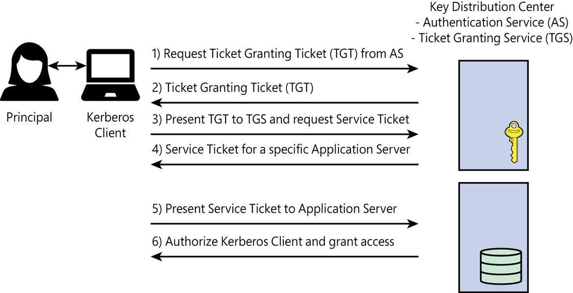
Figure 2-4 How Kerberos authentication works.
The client uses this SPN to request access. After a verification step, the TGS sends a ticket and session key to both the SQL Server and the client, respectively. When the client uses the ticket and session key on the SQL Server, the connection is authenticated by the SQL Server using its own copy of the session key.
For SQL Server to use Kerberos authentication instead of the older NTLM, the Windows domain account that runs the SQL Server service must register the SPN with the domain controller. Otherwise, the authentication will fall back to NTLM, which is far less secure. The easiest way to achieve this is to grant the service account the Write ServicePrincipalName permission in AD DS. To configure an SPN manually, you must use the Setspn.exe tool, which is built into Windows.
Note
You can also manage SPNs using the dbatools PowerShell module, available from https://dbatools.io.
Access other servers and services with delegation
Kerberos delegation enables an application such as SQL Server to reuse end-user credentials to access a different server. This is intended to solve the so-called double-hop issue, in which the TGS verifies only the first hop, namely the connection between the client and the registered server. In normal circumstances, any additional connections (the second hop) would require reauthentication.
Delegation impersonates the client by sending the client’s TGT on the client’s behalf. This in turn causes the TGS to send tickets and session keys to the original server and the new server, allowing authentication. Because the original connection is still authenticated using the same TGT, the client now has access to the second server.
For delegation to work, the service account for the first server must be trusted for delegation, and the second server must be in the same AD forest or between forests with the appropriate trust relationship.
Azure Active Directory
Azure Active Directory (Azure AD) is concerned with identity management for Internet-based and on-premises services, which use HTTP and HTTPS to access websites and web services without the hierarchy associated with on-premises AD.
You can employ Azure AD for user and application authentication—for example, to connect to Azure SQL services or Microsoft Office 365. There are no organizational units or group policy objects. You cannot join a machine to an Azure AD domain, and there is no NTLM or Kerberos authentication. Instead, protocols like OAuth, OpenID Connect (based on OAuth 2.0), SAML, and WS-Federation are used.
You can authenticate (prove who you are), which then provides authorization (permission, or claims) to access certain services, and these services might not be controlled by the service that authenticated you. Think back to network credentials. On an on-premises AD, your user credentials know who you are (your authentication) and what you can do (your authorization).
Protocols like OpenID Connect blur these lines by extending an authorization protocol (what you can do) into an authentication protocol (who you are). This works in a similar manner to Kerberos, whereby an authorization server allows access to certain Internet services and applications, although permissions are granted with claims.
Assert your identity with claims
Claims are a set of “assertions of information about the subject that has been authenticated” (https://learn.microsoft.com/azure/active-directory/develop/access-tokens#claims-in-access-tokens).
Think of your user credentials as a security token that indicates who you are, based on how you were authenticated. This depends on the service you originally connected to (i.e., Facebook, LinkedIn, Google, Office 365, or Twitter).
Inside that user object is a series of properties, or attributes, usually in the form of key-value pairs. The specific attributes, or claims, depend on the authentication service used.
Authentication services like Azure AD might restrict the amount of information permissible in a user object to provide the service or application just enough information about you to prove who you are, and to give you access to the service you’re requesting, without sharing too much about you or the originating authentication service.
Federation and single sign-on
Federation is a fancy word that means an independent collection of websites or services that can share information between them using claims. An authentication service enables you to sign in with one entity (LinkedIn, GitHub, or Microsoft) and then use that identity for other services controlled by other entities.
This is what makes claims extremely useful. If you use a third-party authentication service, that third party will make certain information available in the form of claims (key-value pairs in your security token) that another service to which you’re connecting can access without needing to sign in again, and without that service having access into the third-party service.
For example, suppose you use LinkedIn to sign into a blogging service so you can leave a comment on a post. The blogging service does not have access to your LinkedIn profile, but the claims it provides might include a URL to your profile image, a string containing your full name, and a second URL back to your profile. This way, the blogging service does not know anything about your LinkedIn account, including your employment history, because that information is not in the claims necessary to leave a blog post comment.
Log into Azure SQL Database
Azure SQL Database uses three levels of security to allow access to a database. First is the firewall, which is a set of rules based on origin IP address or ranges and allows connections to only TCP port 1433.
The second level is authentication (proving who you are). You can either connect by using SQL Authentication, with a username and password (like connecting to a contained database on an on-premises SQL Server instance), or Azure AD authentication.
Microsoft recommends using Azure AD whenever possible because it does the following (according to https://learn.microsoft.com/azure/sql-database/sql-database-aad-authentication):
Centralizes user identities and offers password rotation in a single place
Eliminates the storage of passwords by enabling integrated Windows authentication and other forms of authentication supported by Azure AD
Offers token (claims-based) authentication for applications connecting to Azure SQL Database
The third level is authorization (what you can do). This is managed inside the Azure SQL database using role memberships and object-level permissions, and works in a similar way to an on-premises SQL Server instance.
- You can read more about SQL Server security in Chapters 12 and 13.
Kerberos for Azure SQL Managed Instance
Windows Authentication for Azure AD principals, which is in preview as of this writing, enables you to connect traditional on-premises applications to an Azure SQL Managed Instance. You can set up your existing Azure AD tenant as a Kerberos realm. Then, on the AD domain, you create an incoming trust for that Azure AD realm. When a client sends a Kerberos ticket to the Azure SQL Managed Instance, the ticket is exchanged by this feature for an Azure AD token. This allows authentication for Azure AD without providing access to the internal domain.
Understand virtualization and containers
Hardware abstraction has been around for many years. In fact, Windows NT was designed to be hardware independent. We can take this concept even further by abstracting through virtualization and containers.
Virtualization. Abstracts the entire physical layer behind what’s called a hypervisor, or virtual machine manager (VMM), so that physical hardware on a host system can be logically shared between different VMs, or guests, running their own operating systems.
Containers. Abstract away not just the hardware, but the entire operating system as well. Because it does not need to include and maintain a separate OS, a container has a much smaller resource footprint—often dedicated to a single application or service with access to the subset of hardware it needs.
A virtual consumer (a guest OS or container) accesses resources in the same way as a physical machine. As a rule, it has no knowledge that it is virtualized.
Going virtual
The move to virtualization and containers has come about because in many organizations, physical hardware is not being used to its full potential, and systems might spend hundreds of hours per year sitting idle. By consolidating an infrastructure, you can share resources more easily, reducing the amount of waste and increasing the usefulness of hardware.
Certain workloads and applications are not designed to share resources, however, and misconfiguration of shared resources by system administrators might not take these specialized workloads into account. SQL Server is an excellent example of this, because it is designed to use all the physical RAM in a server by default.
If resources are allocated incorrectly from the host level, contention between the virtual consumers takes place. This phenomenon is known as the noisy neighbor, in which one consumer monopolizes resources on the host, which negatively affects the other consumers. With some effort on the part of the network administrators, this problem can be alleviated.
The benefits far outweigh the downsides, of course. You can move consumers from one host to another in the case of resource contention or hardware failure. Some orchestrator software can even do this without even shutting down the consumer.
It is also much easier to take snapshots of virtualized file systems than physical machines, which you can use to clone VMs, for instance. This reduces deployment costs and time when deploying new servers, by “spinning up” a VM template and configuring the OS and the application software that was already installed on that virtual hard drive.
Expanding on the concept of VM templates, you can also get these same benefits using containers. With containers, you can spin up a new container, which includes all the software needed to run an application, based on an image in much the same way.
Note
A container is an image that is composed from a plain text configuration file. Docker containers, for example, are composed using a Dockerfile.
Over time, the benefits become more apparent. New processors with low core counts are becoming more difficult to find. Virtualization makes it possible for you to move physical workloads to virtual consumers (now or later) that have the appropriate virtual core count, and gives you the freedom to use existing licenses, thereby reducing cost.
- David Klee writes more about this in the article “Point Counterpoint: Why Virtualize a SQL Server?” available at http://www.davidklee.net/2017/07/12/point-counterpoint-why-virtualize-a-sql-server.
While there are several OS-level virtualization technologies in use today (including Windows containers), we focus on Docker containers specifically. As for VM hypervisors, there are two main players in this space: Microsoft Hyper-V and VMware.
Provision resources for virtual consumers
Setting up VMs or containers requires an understanding of their anticipated workloads. Fortunately, as long as resources are allocated appropriately, a virtual consumer can run almost as quickly as a physical server on the same hardware, but with all of the benefits that virtualization offers. It makes sense, then, to overprovision resources for many general workloads.
Avoid overcommitting more memory than you have
Suppose you have 10 VMs filling various roles—such as Active Directory domain controllers, DNS servers, file servers, and print servers (the plumbing of a Windows-based network, with a low RAM footprint)—all on a single host with 64 GB of physical RAM.
Each VM might require 16 GB of RAM to perform properly. However, in practice, you have determined that 90 percent of the time, each VM can function with 4 to 8 GB RAM, leaving 8 to 12 GB of RAM unused per VM. You could thus overcommit each VM with 16 GB of RAM (for a total of 160 GB), but still see acceptable performance, without having a particular guest swapping memory to the drive because of low RAM, 90 percent of the time.
For the remaining 10 percent of the time, for which paging unavoidably takes place, you might decide that the performance impact is not sufficient to warrant increasing the physical RAM on the host. You are therefore able to run 10 virtualized servers on far less hardware than they would have required as physical servers.
Caution
Because SQL Server uses all the memory it is configured to use (limited by edition), it is not good practice to overcommit memory for VMs running SQL Server. It is critical that the amount of RAM assigned to a SQL Server VM is available for exclusive use by the VM, and that the Max Server Memory setting is configured correctly (see Chapter 3). This is especially critical if you use the LPIM policy.
Provision virtual storage
In the same way that you can overcommit memory, you can overcommit storage. This is called thin provisioning, in which the consumer is configured to assume that there is a lot more space available than is physically on the host. When a VM begins writing to a drive, the actual space used is increased on the host until it reaches the provisioned limit.
This practice is common with general workloads, for which space requirements grow predictably. An OS like Windows Server might be installed on a guest with 127 GB of visible space, but there might be only 250 GB of actual space on the drive shared across 10 VMs.
For specialized workloads like SQL Server, thin provisioning is not a good idea. Depending on the performance of the storage layer and on the data access patterns of the workload, it is possible that the guest will be slow due to drive fragmentation (especially with storage built on mechanical hard drives), or even run out of storage space. This can occur for any number of reasons, including long-running transactions, infrequent transaction log backups, or a growing tempdb.
It is therefore a better idea to use thick provisioning of storage for specialized workloads. That way, the guest is guaranteed the storage it is promised by the hypervisor, and there is one less thing to worry about when SQL Server runs out of space at 3 a.m. on a Sunday morning.
Note
Most of the original use-cases around containers were web and application server workloads, so early implementations did not include options for persisting data across container restarts. This is why container storage was originally considered to be ephemeral. Now that containers can be used for SQL Server, persistent storage is available using either bind points or named volumes.
When processors are no longer processors
Virtualizing CPUs is challenging, because as discussed earlier in this chapter, CPUs work by having a certain number of clock cycles per second. For logical processors (the physical CPU core plus any logical cores if SMT is enabled), each core shares time slices, or time slots, with each VM. Every time the CPU clock ticks over, that time slot might be used by the hypervisor or any one of the guests.
Just as it is not recommended to overprovision RAM and storage for SQL Server, you should not overprovision CPU cores. If there are four quad-core CPUs in the host (four CPU sockets populated with a quad-core CPU in each socket), there are 16 cores available for use by the VMs, or 32 when accounting for SMT.
Virtual CPU
A virtual CPU (vCPU) maps to a logical core, but in practice, the time slots are shared evenly over each core in the physical CPU. A vCPU is more powerful than a single core because the load is parallelized across each core.
One of the risks of mixing different types of workloads on a single host is that a business-critical workload like SQL Server might require all the vCPUs to run a large, parallelized query. If there are other guests using those vCPUs during that specific time slot and the CPU is overcommitted, those guests will need to wait.
There are certain algorithms in hypervisors that allow vCPUs to cut in line and take over a time slot. However, this results in a lag for the other guests, causing performance issues. For example, suppose a file server has two virtual processors assigned to it. Further assume that on the same host, a SQL Server has eight virtual processors assigned to it. It is possible for the VM with fewer virtual logical processors to “steal” time slots because it has a lower number allocated to it.
There are several ways to deal with this, but the easiest solution is to keep like with like. That is, any guests on the same host should have the same number of vCPUs assigned to them, running similar workloads. That way, the time slots are more evenly distributed, and it becomes easier to troubleshoot processor performance. It might also be practical to reduce the number of vCPUs allocated to a SQL Server instance so that the time slots are better distributed.
Caution
A VM running SQL Server might benefit from fewer vCPUs. If too many cores are allocated to the VM, it could cause performance issues due to foreign memory access because SQL Server might be unaware of the underlying NUMA configuration. Remember to size your VM CPU core allocation as a multiple of a NUMA node size.
The network is virtual, too
Before, certain hardware devices, such as NICs, routers, firewalls, and switches, might have been used to perform discrete tasks. But now, these tasks can be accomplished exclusively through a software layer using virtual network devices.
Several VMs might share one or more physical NICs on a physical host, but because it’s all virtualized, a VM might have several virtual NICs mapped to that one physical NIC.
This enables several things that previously might have been cumbersome and costly to implement. For example, software developers can now test against myriad configurations for their applications without having to build a physical lab environment using all different combinations.
With the general trend of consolidating VMs and containers, virtual networking facilitates combining and consolidating network devices and services into the same environment as these virtual consumers, lowering the cost of administration and reducing the need to purchase separate hardware. You can replace a virtualized network device almost immediately if something goes wrong, vastly reducing downtime.