1. Working with Excel’s Ribbon Menus

In this chapter, you are introduced to Excel’s Ribbon menu and learn the basics of working with workbooks and worksheets. Topics covered in this chapter include
→ Familiarizing yourself with the Ribbon tabs
→ Understanding contextual tabs
→ Understanding workbooks and worksheets
→ Customizing the Quick Access Toolbar
Like any other application, Excel has a basic workspace called the user interface. A user interface is the combination of screens, menus, and icons you use to interact with an application. In Excel, the user interface is primarily composed of the Ribbon menu, workbooks, and worksheets. The Ribbon is the name given to the row of tabs and buttons you see at the top of Excel. The Ribbon’s tabs and buttons bring your favorite commands into the open by showing multiple commands grouped in specific categories.
The Ribbon is made up of five basic components: the Quick Access Toolbar, tabs, groups, command buttons, and dialog launchers.
• The Quick Access Toolbar is essentially a customizable toolbar to which you can add commands that you use most frequently.
• Tabs contain groups of commands that are loosely related to core tasks. Actually, it helps to think of each tab as a category.
• Groups contain sets of commands that fall under the umbrella of that tab’s core task. Each group contains buttons, which you click to activate the command you want to use.
• Dialog launchers are activated by clicking the small arrow located in the lower-right corner of certain groups. Clicking any dialog launcher activates a dialog box containing all the commands available for a given group.
Familiarizing Yourself with the Ribbon Tabs
Each tab on the Ribbon contains groups of commands loosely related to a central task. Don’t be alarmed by the number of commands on each tab. As you go through this book, you’ll quickly become familiar with each of the common Excel commands. For now, take some time to become familiar with each of Excel’s default tabs (the way they are set up before you customize it to fit your working needs).
1. Click the Home tab. This tab contains commands for common actions such as formatting, copying, pasting, inserting, and deleting columns and rows.
2. Click the Insert tab. This tab contains commands that enable you to insert objects such as charts and shapes into your spreadsheets.
3. Click the Page Layout tab. This tab holds all the commands that enable you to determine how your spreadsheet looks, both onscreen and when printed. These commands control options such as theme colors, page margins, and print area.
4. Click the Formulas tab. This tab holds all the commands that help define, control, and audit Excel formulas.

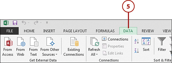
5. Click the Data tab. This tab features commands that enable you to connect to external data, as well as manage the data in your spreadsheet.
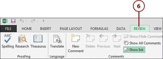
6. Click the Review tab. With commands such as Spell Check, Protect Sheet, Protect Workbook, and Track Changes, the theme of the Review tab is protecting data integrity in your spreadsheet.
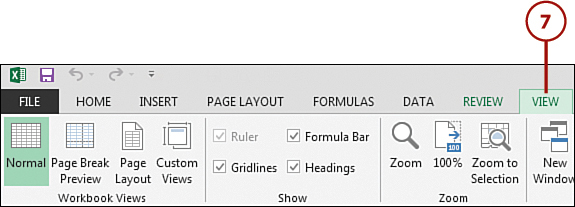
7. Click the View tab. The commands on this tab are designed to help you control how you visually interact with your spreadsheet.
8. The File tab exposes the Backstage view, where you find commands to help you open existing Excel workbooks, create new workbooks, save workbooks, apply protection, and much more. Chapter 2, “Managing Workbooks and Worksheets,” covers the File tab in detail.

If you feel the Ribbon takes up too much space at the top of your screen, you can minimize it—that is to say, you can hide the Ribbon and show only the tab names. To do this, simply right-click the Ribbon and select Unpin the Ribbon. At this point, the Ribbon becomes visible only if you click on a tab. To revert back to the default Ribbon view, right-click the Ribbon, and click the Unpin the Ribbon toggle.
Understanding Workbooks and Worksheets
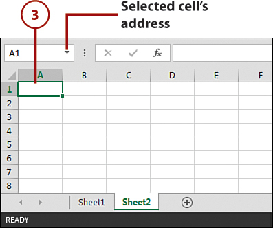
An Excel file, often referred to as a workbook, contains one or more spreadsheets, or worksheets. Each box in the worksheet area is referred to as a cell. Each cell has a cell address, which is composed of a column reference and a row reference. The letters across the top of the worksheet make up the column reference. The numbers down the left side of the worksheet make up the row reference. For example, the address of the top, leftmost cell is A1. This is because the cell is located at the intersection of the A column and row 1.
By default, Excel 2013 opens a new workbook with one blank worksheet. You can add, delete, and rename worksheets within a workbook, as needed.
Explore Worksheets
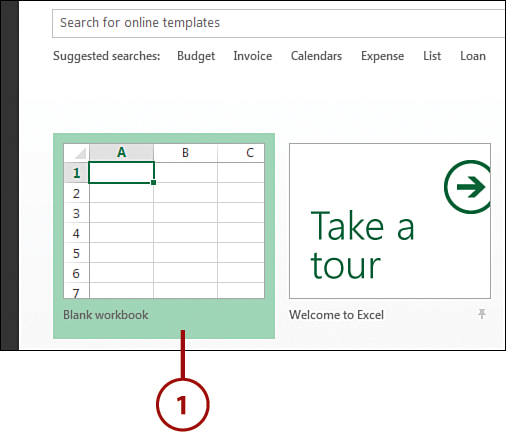
1. Open Excel and open a new Blank workbook.
2. The workbook opens with one worksheet called Sheet1. This worksheet contains cells you can use to start entering and editing data.
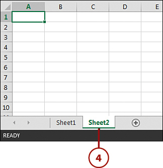
3. Click the plus icon to add a new worksheet.

4. The new worksheet is added and named Sheet2. Each time you add a worksheet, Excel gives the worksheet a default name of Sheet XX, where XX is the next sequential number.
Workbooks and Worksheets in Depth
You read more about managing workbooks and worksheets in detail in Chapter 2.
Explore Columns, Rows, and Cells
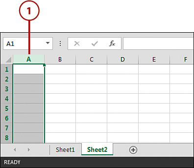
1. Click the column reference and observe how the entire column is selected.
2. Click the row reference and observe how the entire row is selected.

3. Click the cell intersecting at column A and row 1. You can select a single cell on the worksheet area.
The Big Grid
Excel 2013 has 1,048,576 rows and 16,384 columns. This means that there are more than 17 billion cells in a single Excel worksheet. So what happens if you need more than 1 million rows and more than 16,000 columns? Well, the short answer is that you’ll have to start a new worksheet.
Understanding Contextual Tabs
Contextual tabs are special types of tabs that appear only when a particular object is selected, such as a chart or a shape. These contextual tabs contain commands specific to whatever object you are currently working on.
For example, after you add a shape to a spreadsheet, a new Format tab appears. This is not a standard tab, but a contextual tab—meaning it activates only when you work with a shape.
Follow the steps in this task to add a shape and view the contextual tab.
Work with Contextual Tabs
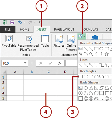
1. Open Excel and start a new blank workbook (as described earlier in the “Explore Worksheets” task). When the new workbook is open, click the Insert tab.
2. Click the Shapes command button.
3. Click the rectangle shape in the menu of shapes.
4. Click anywhere on your spreadsheet to embed your selected shape.
All Shapes and Sizes
Read more about shapes and other graphics in Chapter 7, “Working with Graphics.”
5. Click your new shape to select it, and you see the contextual tab, labeled Format, that appears any time the shape is selected.

Customizing the Quick Access Toolbar
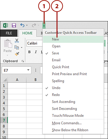
The small buttons at the top-left side of the Excel screen are known collectively as the Quick Access Toolbar. By default, the Quick Access Toolbar contains three commands: Save, Undo, and Redo. If you click the drop-down selection arrow next to the Redo button on the Quick Access Toolbar, you see that these 3 commands are only 3 of 11 available as prebuilt or built-in options. Placing a check next to any of the options that you see here automatically adds each option to the Quick Access Toolbar. So, clicking New adds the New command, and clicking Open adds the Open command. You can actually click each one of these and have all 11 options available to you in the Quick Access Toolbar. In the tasks that follow, you find out how to add commands to the Quick Access Toolbar to customize it to fit your workflow.
Add a Command to the Quick Access Toolbar
Follow these steps to add to the Quick Access Toolbar one of the commands available from the drop-down menu.
1. Click the arrow to open the Quick Access toolbar drop-down to see all the existing commands you can add.
2. Click the New command to add it to the Quick Access toolbar.
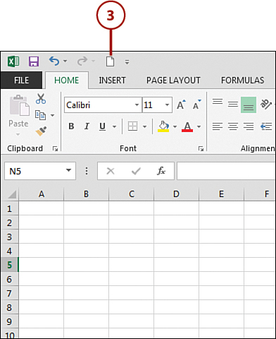
3. You now have a New icon on your Quick Access toolbar.
Moving the Quick Access Toolbar
You can move the Quick Access Toolbar under the Ribbon by right-clicking its drop-down arrow and selecting Show Below the Ribbon. This moves the entire Quick Access Toolbar under the Ribbon—closer to your worksheet.
Add Other Commands to the Quick Access Toolbar
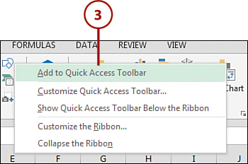
You’re not limited to only the commands available on the Quick Access Toolbar drop-down menu—you can add all kinds of commands. For example, if you often work with shapes, you can add the Shapes command to the Quick Access Toolbar.
1. Click the Insert tab.
2. Right-click the Shapes command button.

3. Click the Add to Quick Access Toolbar menu item.
Adding Entire Groups
You can add entire groups to your Quick Access Toolbar. For instance, if you often use the Illustrations group on the Insert tab, you can right-click that entire group and select the Add to Quick Access Toolbar option.
Add Hidden Commands to the Quick Access Toolbar
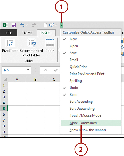
A closer look at the drop-down menu next to the Quick Access Toolbar reveals an option called More Commands. When you click this item, the Excel options dialog box opens up with the Quick Access Toolbar panel activated. This panel enables you to select from the entire menu of Excel commands, adding them to your Quick Access Toolbar. This comes in handy if you want to add some of the more obscure Excel commands that aren’t found on the Ribbon.
1. Click the Quick Access Toolbar drop-down arrow.
2. Select the More Commands option.
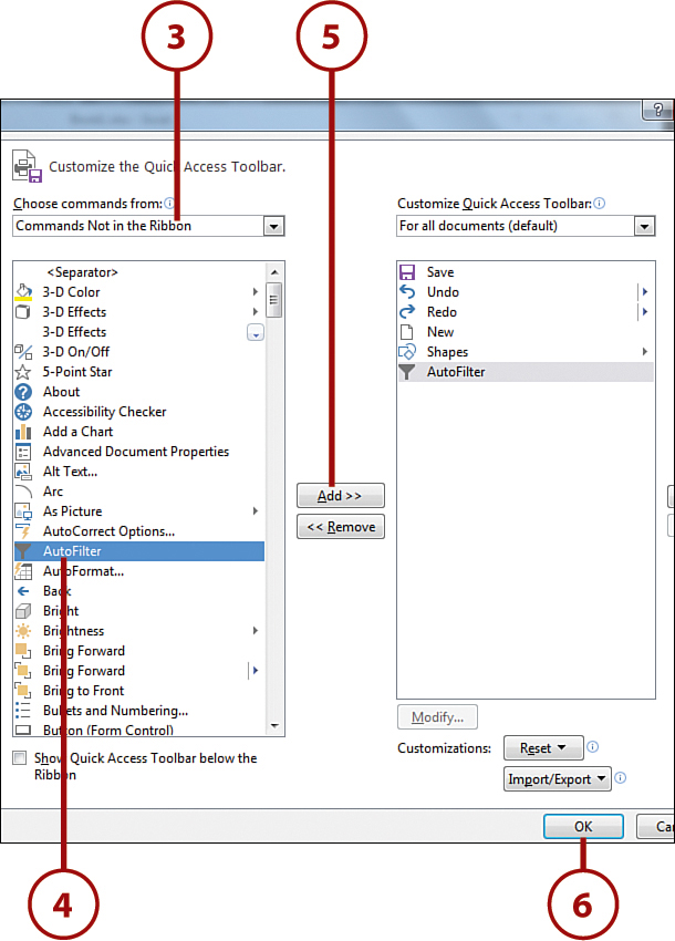
3. Choose Commands Not in the Ribbon.
4. Find and select the AutoFilter command.
5. Click the Add button.
6. Click OK to add the command to the Quick Access Toolbar.
Removing Commands
To remove a command from the Quick Access Toolbar, simply right-click it and select the Remove from Quick Access Toolbar option.