Chapter 6. Balances in Open Systems
In Chapters 3 (Section 3.4) and 4 we applied the first and second law to closed systems. Most chemical processes involve open systems that exchange mass with the surroundings, usually in the form of flow streams. These streams carry with them not only mass, but also energy and entropy. The application of the first and second law to open systems must, therefore, account for energy and entropy exchanges that take place through flow streams. A flow process may operate under steady-state or unsteady conditions. Under steady state, all properties at any given point are constant and do not vary with time (though they may vary from one point of the process to another). Steady state is the preferred mode of operation because it leads to continuous production and is simpler to maintain control. Nonetheless, unsteady-state conditions are also encountered, either during start-up and shut-down of a continuous process, or in batch processes that are designed to operate in discrete cycles. In this chapter we apply the first and second law to open systems that involve flow streams. The most general form of these balances is the unsteady-state form, from which steady state is obtained as a special condition. We then apply the energy and entropy balance to various common units encountered in chemical processes, as well as to larger processes involving multiple units. The learning objectives for this chapter are to:
1. Develop the balance equation for energy and entropy in open systems.
2. Obtain the steady-state equation as a special case of the general unsteady state balance.
3. Perform thermodynamic analysis on individual process units such as heat exchanger, turbines, pumps, compressors, and throttling valves.
4. Apply the first and second law to solve the material and energy balances in flow sheets that involve multiple units, and to analyze the operation of the process in terms of irreversible features and overall efficiency of energy utilization.
5. Perform thermodynamic analysis and preliminary design of power cycles and refrigeration units.
6. Learn to use various thermodynamic charts such as the entropy-temperature, enthalpy-entropy and enthalpy-pressure charts to perform graphical calculations of various units and processes.
6.1 Flow Streams
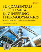
An open system exchanges mass with its surroundings. Most commonly this exchange takes place through flow streams, usually pipes, that carry material into and out of the system. Mass exchange does not have to occur through pipes. For example, the free surface of a liquid (or of an ocean) may exchange mass with the gas above it through evaporation, condensation, or absorption. However, in their majority, the situations we will encounter involve flow through pipes. Figure 6-1 gives a partial list of some common flow units encountered in chemical processes, which will be discussed in more detail in this chapter.
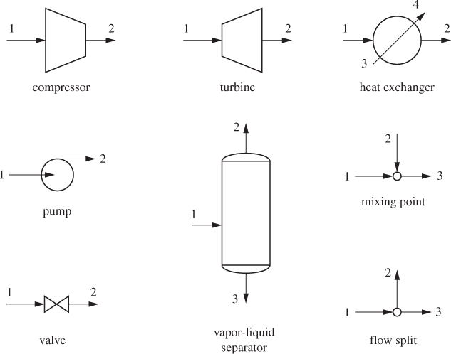
Figure 6-1: Schematic representation of some common flow equipment.
The mass flow rate in a stream will be denoted as ![]() (kg/s), with the dot indicating “rate per unit time.” Given the mass flow rate, the mass (in kg) that flows in time dt
(kg/s), with the dot indicating “rate per unit time.” Given the mass flow rate, the mass (in kg) that flows in time dt
When mass flows through a pipe, the mass flow rate can be expressed in terms of the mean velocity1 of the fluid in the pipe:
1. The flow inside a pipe is not uniform because the fluid at the center of the pipe moves faster than the fluid near the pipe walls. The velocity profile in pipes is a subject of fluid mechanics. Here, we avoid such complicating factors by considering the average velocity of the fluid over the entire cross section of the pipe.
where v is the average velocity (m/s), a is the cross-sectional area of the pipe (m2), d is the mass density (kg/m3), and V is the specific volume (m3/kg). Suppose a stream with mass flow rate ![]() exchanges the amount of heat, Q, or shaft work, Ws, per kg of fluid (i.e., the units of Q and Ws are J/kg). The rate of the energy exchange is
exchanges the amount of heat, Q, or shaft work, Ws, per kg of fluid (i.e., the units of Q and Ws are J/kg). The rate of the energy exchange is
with units of J/s, or W (watt). The amount of heat or work that is transferred within time dt is,
In the general case, the exchange rates ![]() ,
, ![]() , and
, and ![]() will vary with time. At steady state, however, all rates constant and do not vary with time.
will vary with time. At steady state, however, all rates constant and do not vary with time.
6.2 Mass Balance
Mass is a conserved quantity,2 therefore, all the mass that crosses the boundaries of a system must be accounted for. All conserved quantities satisfy the general balance equation,
2. We are excluding the possibility of mass-to-energy conversions by nuclear reaction.
The term accumulation is to be understood to represent either built up, if positive, or depletion, if negative. This balance equation applies at all times, including a small time interval dt. Consider the process shown in Figure 6-2. The system is defined by the dashed line and includes several interconnected units. For the purposes of computing the overall balance in the system, the internal details of the process are unimportant. What is important to know are the exchanges that cross the system boundaries. In the case of mass, such exchange takes place only through flow streams: mass enters through streams 1 and 2, and exits through streams 3 and 4. Applying eq. (6.7) to the system over a small time interval dt, we have
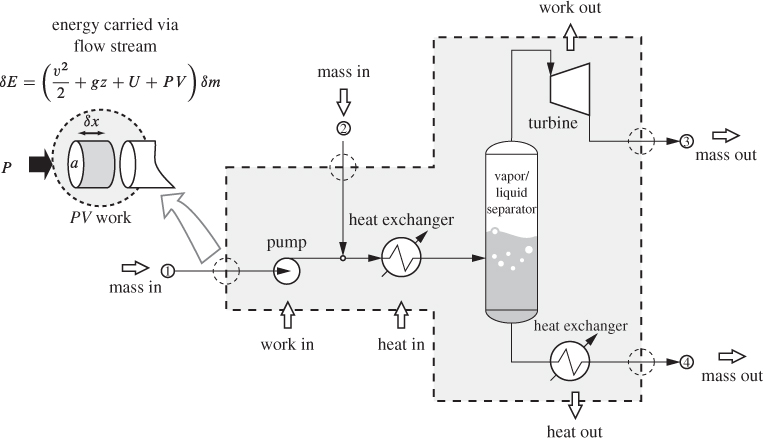
Figure 6-2: Setup for the energy balance in open system. The system is defined by the dashed line around it.
dm1 + dm2 − dm3 − dm4 = dMtot
where dMtot refers to the change in the total mass contained within the system. We divide by dt and note that the terms on the left-hand side give the flow rates of the corresponding streams:
We rewrite this result in the general and more compact form,

where ![]() is shorthand for
is shorthand for
and the summations are understood to go over all inlet and outlet flow streams. Equation (6.8) expresses the unsteady-state mass balance in terms of rates, and states that the net rate at which mass enters the system is equal to the rate at which mass accumulates inside the system. At steady state, the accumulation term is by definition zero. The steady-state form of the material balance then is,
or
This result indicates that at steady state the amount of mass that enters the system is exactly equal to the amount that exits.
Note
The Operator Δ(···)
In Chapter 3 we introduced the operator Δ to mean “final minus initial.” Here, we encounter a more general interpretation of this operator, to mean “the sum of all that goes out (via flow streams) minus the sum of all that comes in.” If we imagine the observer to move with the fluid, inlets represent the state “before” and outlets the state “after.” This interpretation of the operator applies to all extensive properties, including energy and entropy.
6.3 Energy Balance in Open System
As a conserved quantity, energy obeys the general balance equation in eq. (6.7). To construct this equation we must first identify all the exchanges of energy between system and surroundings. We begin by noting that a flow system may exchange heat and shaft work with the surroundings. Heat is exchanged via heat exchangers; shaft work can be exchanged in a number of units, for example, pumps, compressors, turbines, and the like. These units will be considered in more detail later. Here, and for the purposes of constructing the overall energy balance of the process, we will take the total (net) amount of heat that is exchanged to be ![]() , and the total (net) amount of shaft work to be
, and the total (net) amount of shaft work to be ![]() . Exchanges are defined with the usual sign convention: they are positive if they enter the system, negative if they exit. Based on this convention, the heat and work must be counted as part of the energy that goes “in.” Over a time interval dt, these amounts are
. Exchanges are defined with the usual sign convention: they are positive if they enter the system, negative if they exit. Based on this convention, the heat and work must be counted as part of the energy that goes “in.” Over a time interval dt, these amounts are
Since mass carries with it energy in various forms, energy is also exchanged via flow streams. In general, mass carries kinetic, potential and internal energy. Kinetic energy is due to the velocity of the fluid; potential energy due to gravity enters through the elevation of individual streams (not all pipes need to be at the same height); internal energy is of course an inseparable part of matter. The combined kinetic, potential, and internal energy that is carried by a mass dm, over a time interval dt, is
where v is the mean velocity in the pipe z is the elevation with respect to a reference plane, and U is the specific internal energy of the fluid at the pressure and temperature of the particular location. There is an additional energy contribution that is not immediately obvious: to introduce this element of mass into the system, we must push from the outside against the pressure P of the fluid at this point and this requires work. This requires an amount of work that must be included in the balance. To calculate this work, we assume for simplicity that the pipe has a circular cross section with area a. The mass dm then has the shape of a cylindrical plug with length dx. The force that opposes this volume element is equal to the product of the pressure times the cross section of the element, Pa, and this force must be displaced by a distance dx. The required amount of work is
dW′ = (Pa)dx = P(a dx).
The product a dx is the volume of the plug and this may be expressed in terms of the specific volume, V:
a dx = Vdm.
Combining these results, the amount of work needed to push the mass element, dm, into the system is
dW′ = PV dm.
We recognize this as a form of PV work and note that it depends on the state (pressure, specific volume) at the point of entry. For inlet streams, this represents work that is done by the surroundings; for outlet streams, it is work that is done by the system. To summarize these calculations, the energy that is carried by a mass dm via flow steams is
In the last equation we used the definition of enthalpy to combine U and PV into a single term. The net amount of energy that goes into the system is obtained by combining eqs. (6.12) and (6.14):
This net energy must be accounted for by the accumulation of energy inside the system. The accumulation is represented by the change of the total amount of internal energy in the system:3
3. In principle, a system may also accumulate kinetic, potential, or any other type of energy. Accumulation of kinetic or potential energy means that the velocity or the vertical elevation of the system changes, as in a roller coaster, or in a rocket. These modes of energy accumulation are not relevant to stationary processes such as those considered here. This leaves internal energy as the only accumulation term.
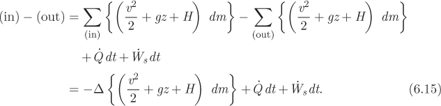
We equate the results in eqs. (6.15) and (6.16), divide both sides by dt, replace the ratio dm/dt by flow rate of the stream, ![]() , and write the final result in the form:
, and write the final result in the form:
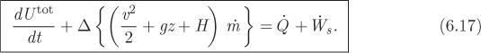
This equation gives the general unsteady-state energy balance equation in an open system. It is often referred to as the form of the first law for open systems. Below we consider a number of special cases.
Special Case: Closed System
The closed system may be considered as a special case of an open system in which all flow streams have zero flow. This means that if the mass flows are turned off, eq. (6.17) must revert to the familiar expression for a closed system. Let us confirm this result. With all mass flow rates set to zero, eq. (6.17) becomes
Multiplying both sides by dt, this becomes,
This is precisely the form of the first law for a closed system of constant volume that exchanges heat and shaft work with the surroundings (see eq. [3.10]). The reason that the PV work does not appear here is that the form of the energy balance in eq. (6.17) implicitly assumes that the system has constant volume, i.e., its boundaries are rigid and thus the system is prevented from exchanging any PV work. For an open system with movable boundaries (a rubber balloon, for example), eq. (6.17) must be amended to include PV work in addition to any shaft work.
Special Case: Steady State
For a process at steady state, the accumulation term is zero and the energy balance simplifies to
It will often be the case that the contribution of kinetic and potential energy terms is much smaller than the contribution of the other terms. Whenever this is true, the steady-state energy balance is further reduced to
where the operator Δ (![]() ) is understood to mean the sum of the quantity
) is understood to mean the sum of the quantity ![]() over all outlet streams minus the sum of the same quantity over all inlet streams. If the process has a single inlet and a single outlet stream, their mass flow rates at steady state must be equal (see eq. [6.10]). Equation (6.19) then becomes
over all outlet streams minus the sum of the same quantity over all inlet streams. If the process has a single inlet and a single outlet stream, their mass flow rates at steady state must be equal (see eq. [6.10]). Equation (6.19) then becomes
where ![]() is the common value of the flow rate. Dividing both sides by
is the common value of the flow rate. Dividing both sides by ![]() and using eqs. (6.3) and (6.4), this result becomes
and using eqs. (6.3) and (6.4), this result becomes
where ΔH = H2 − H1. This simplified form of the energy balance applies to steady-state processes with two streams (one inlet, one outlet), provided that kinetic and potential energy contributions are negligible.
6.4 Entropy Balance
Entropy is not a conserved quantity. The entropy of the universe increases as a result of irreversible processing, and the balance equation must be amended to include a generation term. We must also keep in mind that such equation must be applied, not to the system alone, but to the universe. Accordingly, the entropy balance must be written for the system and the surroundings. With these considerations in mind we return to the system shown in Figure 6-2. The starting equation is the second law, according to which entropy generation is the sum of the entropy change of the system and the surroundings:
We now consider all changes in entropy over a short time dt. For the entropy change of the system we simply write,
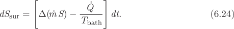
where dStot (we will drop the subscript “sys”) is the accumulation of entropy within the system. The entropy change of the surroundings has two contributions. One is through flow streams: streams 1 and 2 exit the surroundings taking entropy with them; streams 3 and 4 enter the surroundings, adding to their entropy. The entropy change due to these flows is
where Si is the specific entropy of stream i and ![]() dt is the corresponding amount of mass that flows through that stream in time dt. The second contribution to the entropy change of the surroundings comes from interactions with baths. Suppose for simplicity that all the heat that is exchanged between the system and the surroundings comes from a single bath at temperature Tbath. The amount of heat exchanged in time dt is
dt is the corresponding amount of mass that flows through that stream in time dt. The second contribution to the entropy change of the surroundings comes from interactions with baths. Suppose for simplicity that all the heat that is exchanged between the system and the surroundings comes from a single bath at temperature Tbath. The amount of heat exchanged in time dt is ![]() dt (with the sign of
dt (with the sign of ![]() based on the system), and the entropy change is
based on the system), and the entropy change is
The entropy change of the surroundings is the sum of the above contributions:

which we write in the more compact form as
The entropy generation is obtained by adding the contributions of the system and the surroundings:
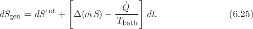
Dividing both sides by dt, this becomes
where ![]() stands for the rate of entropy generation, dSgen/dt. Equation (6.26) is the general unsteady-state entropy balance equation for a flow process that exchanges heat with a bath. If the system exchanges heat with several baths, then an additional term of the form
stands for the rate of entropy generation, dSgen/dt. Equation (6.26) is the general unsteady-state entropy balance equation for a flow process that exchanges heat with a bath. If the system exchanges heat with several baths, then an additional term of the form ![]() must be included for each bath. The general form of this equation is similar to the energy balance, eq. (6.17), with the notable difference4 that the entropy balance contains a generation term. This term represents production of entropy and obeys the inequality of the second law,
must be included for each bath. The general form of this equation is similar to the energy balance, eq. (6.17), with the notable difference4 that the entropy balance contains a generation term. This term represents production of entropy and obeys the inequality of the second law,
4. Also notice that shaft work does not appear explicitly in this equation. It is taken into account indirectly, through its effect on heat and the entropy of the streams.
In the special case of reversible process the generation term is zero and the above relationship becomes an exact equality. Two special forms of the entropy balance are examined below
Steady-State Process
At steady state the accumulation term dStot/dt is zero and the entropy equation can be solved for the generation term:
The first term on the right-hand side is the entropy change of the fluid during a pass trough the process; the second term is the entropy change of the bath during the same time. At steady state, the sum of the two constitutes the entropy change of the universe.
Reversible Adiabatic Process
For a reversible adiabatic process, ![]() and
and ![]() . The entropy balance then reduces to
. The entropy balance then reduces to
In this case, the entropy of the system is a conserved quantity (compare this equation with eq. [6.8] for the mass) since a reversible adiabatic process is also isentropic. In the special case of steady state, this result further simplifies to
which states that the total entropy of the inlet streams is equal to the entropy of the outlet streams.
In typical calculations involving irreversible processes, the unknown quantity is the entropy generation. This may be obtained from the entropy balance once the material and energy balances have been performed and the states of all streams are known. In the special case of reversible process, the rate of entropy generation is known (![]() ) and the entropy balance may be used as an additional equation in the calculation of the unknown quantities of the process.
) and the entropy balance may be used as an additional equation in the calculation of the unknown quantities of the process.
Note
Steady State versus Equilibrium
It is important to distinguish between steady state and equilibrium. In steady state, all accumulation terms (mass, energy, entropy) are equal to zero:
In strict equilibrium, the entropy generation and all exchanges between system and surroundings are zero:
The steady-state condition requires the rate of all exchanges (![]() ,
, ![]() , etc.) to be constant. Accordingly, the rate of entropy production at steady state,
, etc.) to be constant. Accordingly, the rate of entropy production at steady state, ![]() , is also constant but not necessarily zero, unless the process is reversible. A system in strict equilibrium produces no entropy and undergoes no changes in time with respect to any of its properties. For such system, the entropy generation, all accumulation terms, and the rate of all exchanges (
, is also constant but not necessarily zero, unless the process is reversible. A system in strict equilibrium produces no entropy and undergoes no changes in time with respect to any of its properties. For such system, the entropy generation, all accumulation terms, and the rate of all exchanges (![]() ,
, ![]() , etc) are zero. A reversible process produces no entropy (
, etc) are zero. A reversible process produces no entropy (![]() ) and may operate either at steady state (zero accumulation) or at unsteady state (nonzero accumulation):
) and may operate either at steady state (zero accumulation) or at unsteady state (nonzero accumulation):
By strict equilibrium we mean a state of permanent equilibrium in which there is no exchange of mass or energy between system and surroundings. This is to be contrasted with the reversible (quasi-static) process, which is allowed to exchange mass and energy with its surroundings, albeit under slow, quasi-equilibrium conditions, such that the entropy generation is zero.
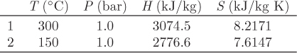
Solution The entropy balance of adiabatic steady-state process is given by eq. (6.28) with ![]() . The mass flow rate of the inlet and outlet streams are equal (by virtue of the steady-state condition on the mass balance equation); therefore, the entropy balance becomes
. The mass flow rate of the inlet and outlet streams are equal (by virtue of the steady-state condition on the mass balance equation); therefore, the entropy balance becomes
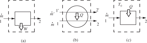
Figure 6-3: Processes with entropy generation (see examples in text): (a) work production in open system; (b) heat exchange between streams; (c); heat exchange between a stream and a heat bath whose temperature is T0.
Entropy generation. This is a steady-state adiabatic process and the entropy balance is given by eq. (6.28) with ![]() :
:

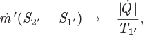
and the temperature of stream 2′ is obtained from the known enthalpy and pressure of the stream. However, when the flow rate of stream 1′2′ is very large (![]() ), we have, H2′ → H1′, and also T2′ → T1. That is, the flow rate is so high that stream 2′ exits practically at the same temperature as the inlet stream. It further follows that the entropy of the exit stream is S2′ → S1′. This poses a numerical difficulty because the quantity
), we have, H2′ → H1′, and also T2′ → T1. That is, the flow rate is so high that stream 2′ exits practically at the same temperature as the inlet stream. It further follows that the entropy of the exit stream is S2′ → S1′. This poses a numerical difficulty because the quantity ![]() (S2′ − S1′), needed in the calculation of entropy generation, is indeterminate:
(S2′ − S1′), needed in the calculation of entropy generation, is indeterminate:
6.5 Ideal and Lost Work
In Chapter 4 we introduced the ideal and lost work for a closed system. Now we extend these concepts to open systems. We return to the generic process in Figure 6-2, which we assume to run at steady state. The process exchanges a net amount of heat ![]() and a net amount of shaft work,
and a net amount of shaft work, ![]() , with its surroundings. As we did in Chapter 4, we will use a single reservoir at temperature T0 as the source and sink for all heat transfers between the system and the surroundings. The steady-state energy and entropy balance equations are
, with its surroundings. As we did in Chapter 4, we will use a single reservoir at temperature T0 as the source and sink for all heat transfers between the system and the surroundings. The steady-state energy and entropy balance equations are
Eliminating the heat term between the two equations we obtain the following expression for the work:
This equation gives the amount of work involved in converting the input streams into output streams. The term ![]() is positive and represents the lost work:
is positive and represents the lost work:
Just as in the case of closed system, it represents a penalty: it increases the work that must be consumed, if the process requires work, and reduces the amount of work that is extracted, if the process produces work. This penalty disappears only if the process is conducted reversibly. The reversible work is obtained from eq. (6.33) with ![]() :
:
It represents the maximum amount of work that can be extracted, or the minimum that must be consumed, in order to convert the input streams into output.
100 MW + 210 MW = 310 MW.
Solving for ![]() we obtain
we obtain

where ![]() (H3 − H1) is the heat with respect to stream 1. The numerical calculations are shown below for each of the two cases.
(H3 − H1) is the heat with respect to stream 1. The numerical calculations are shown below for each of the two cases.
Using ice: The amount of heat ![]() is
is
H3 − H2 = CP(T3 − T2) = (4.18 kJ/kg K)(303.15 − 298.15) (K) = 20.9 kJ/kg.

6.6 Thermodynamics of Steady-State Processes
Chemical processes consist of interconnected unit operations such as heat exchangers, pumps and compressors, separation units, chemical reactors. Generally these are flow systems with several streams carrying mass into and out of a unit. To perform mass and energy balances in such units we will apply the principles developed in the previous chapter. The units we will consider in this chapter are: heat exchangers, compression devices (pumps, gas compressors) and expansion devices (turbines and throttling valves). We will not consider chemical reactors or separation units. These are treated with the same general tools developed in the previous chapter but they require the calculation of mixture properties, which is covered in Part II. Fairly complex processes can be designed by putting together simple units; we will discuss in more detail the preliminary design of power plants, refrigerators and liquefaction processes. By “preliminary” design we refer to the calculation of the mass and energy balances of the process. As we will see, this calculation is straightforward and requires very little information about the inner workings of the device under consideration.
Flow through Pipe
The most basic process is flow of a fluid through a pipe. When a fluid flows in a pipe its motion is resisted by the viscosity of the fluid, which represents molecular “friction” between adjacent layers of fluid that move at different velocities, and also resistance from the walls, which do not move. Viscosity and wall friction represent irreversibilities that dissipate the energy of the fluid into internal energy. To maintain steady flow through a pipe, we must apply mechanical work, usually via a pump. Here we are concerned with the macroscopic energy balance that accounts for changes in the various energy terms between the inlet and outlet of the pipe. Viscosity represents a microscopic mechanism which we will not consider explicitly except as a source of entropy generation. The pipe need not be cylindrical or have constant cross section. It may also span different elevations between inlet and outlet. We will assume that the velocity of the fluid is uniform at all points on a cross section. In reality, fluid velocity near the center of a pipe is faster than near the walls. By ignoring this variation we are dealing the average velocity of the fluid through the cross section. This average velocity is defined in terms of the mass flow rate (see also eq. [6.2]), as
where V is the specific volume of the fluid, ![]() is the mass flow rate, and a is the cross-sectional area of the pipe. Noting that the product V
is the mass flow rate, and a is the cross-sectional area of the pipe. Noting that the product V![]() is equal to the volumetric flow rate (m3/s), the mean velocity is simply equal to this rate divided by the cross-sectional area.
is equal to the volumetric flow rate (m3/s), the mean velocity is simply equal to this rate divided by the cross-sectional area.
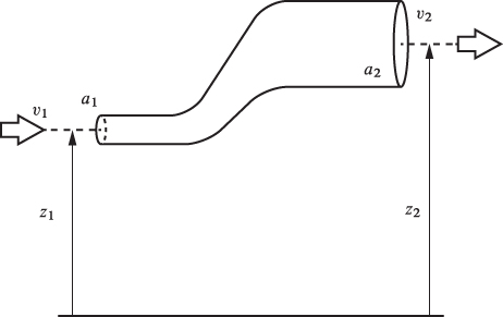
Figure 6-4: Schematic for the calculation of energy losses in flow through a pipe.
We consider now steady-state flow through a pipe, as shown schematically in Figure 6-4. The system may exchange work if a pump is present. To maintain the isothermal condition we must allow for the exchange of heat. Without such exchange, the dissipation of energy into internal energy via viscosity and wall friction would result in a temperature rise. To maintain the system at constant temperature T we will assume that heat is exchange with a bath with the same temperature as the fluid, Tbath = T. Since both the velocity and elevation change (the velocity changes due to variations of the cross-sectional area), kinetic and potential energy will be included. The steady-state energy balance is
Here, Δ(···)12 signifies the difference between inlet and outlet of the quantity in parenthesis. Since we are dealing with one stream at a steady state, the inlet and outlet have the same mas flow rate, ![]() . Dividing both sides by
. Dividing both sides by ![]() we obtain,
we obtain,
The corresponding entropy balance at steady state is

where we used the fact that the heat bath is at the temperature of the system. We divide both sides by ![]() and solve for Q:
and solve for Q:
Q = TΔS12 − TSgen
Substituting this result into the energy balance, eq. (6.37), gives
Recall eq. (5.14), which relates enthalpy and entropy in differential form:
We integrate the above differential from inlet to outlet under constant temperature,
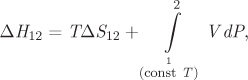
and substitute the result into (6.38):
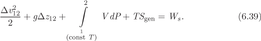
This equation now expresses the macroscopic energy balance for isothermal flow in a pipe. It may further be simplified in the special case of an incompressible fluid. In this case V is constant and the energy balance equation becomes
This form of the mechanical balance is known as the Bernoulli equation. It applies to incompressible fluids and approximately to compressible gases as long as the pressure does not vary much. The Bernoulli equation gives the mechanical work that is required to produce the desired change in velocity, elevation, and pressure between the inlet and outlet of the pipe. The term TSgen represents losses due to irreversibilities that arise from viscosity and wall friction. Its dependence on the viscosity of the fluid, the type of flow (laminar, turbulent), and the roughness of the walls is the subject of fluid mechanics and we will not consider them here in any detail. The main point we wish to make here is that these microscopic mechanisms result in dissipation of the mechanical energy of the fluid into internal energy. To see this, consider a horizontal segment of pipe (Δz12 = 0) with constant cross section (![]() ) that does not include any pumps (Ws = 0). Since Sgen is positive, the exit pressure must be lower than the inlet pressure. This pressure drop arises from the resistance to the flow due to viscosity and wall friction. Therefore, to maintain flow at sufficient pressure, it is necessary to supply work via a pump.
) that does not include any pumps (Ws = 0). Since Sgen is positive, the exit pressure must be lower than the inlet pressure. This pressure drop arises from the resistance to the flow due to viscosity and wall friction. Therefore, to maintain flow at sufficient pressure, it is necessary to supply work via a pump.

ΔP = (100 m)(0.0285649 bar/m) = 2.85 bar.
The entropy generation is calculated from the Bernoulli equation. We set Δz12 = 0 (the pipe is horizontal) and Ws = 0 (there is no pump in this segment of the pipe). Ignoring the slight change of specific volume due to the pressure drop, we will also set ![]() . Then, the entropy generation is
. Then, the entropy generation is
Comments The pressure drop is indeed small, 0.0285 bar per m of pipe length. Of course, given enough length, the pressure drop will be significant. Pressure drop also increases with increasing flow rate, as we can confirm by repeating the calculation with a higher value of ![]() . Other factors that contribute to pressure drop are elbows, valves, and other common elements of piping networks that offer resistance to flow. In general, however, the pressure drop due to flow is rather small, from the point of view that its contribution to the energy balance is small compared to that of heat exchangers, compressors, and the like. In this example, the work equivalent of the frictional losses is
. Other factors that contribute to pressure drop are elbows, valves, and other common elements of piping networks that offer resistance to flow. In general, however, the pressure drop due to flow is rather small, from the point of view that its contribution to the energy balance is small compared to that of heat exchangers, compressors, and the like. In this example, the work equivalent of the frictional losses is
TSgen = (673.15 K)(4.930 J/kg K) = 3.319 kJ/kg.
Adiabatic Mixing
The simplest way to combine streams is by bringing two or more pipes together. This is indicated as a mixing point on the process flow diagram (see Figure 6-5). For practical reasons the pressure of all streams around the mixing point is the same to avoid back flow from a high pressure stream into one at lower pressure. In some cases, mixing takes place inside a tank with or without stirring. In adiabatic mixing, no heat is exchanged between the streams and the surroundings. As a result, the temperature of the outlet stream must change to accommodate the energy of the inlet streams. The steady-state balance equation for adiabatic mixing with no shaft work is
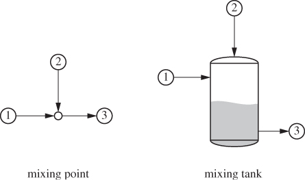
Figure 6-5: Adiabatic mixing of streams.
and the entropy balance is
Mixing is an irreversible process, as the streams that are combined will generally have different temperatures. In the special case that the temperature of all inlet streams is the same (recall that all streams have the same pressure), then all streams, including the exit stream, have the same intensive properties and the entropy generation is zero.
H1 = 83.92 kJ/kg, S1 = 0.2965 kJ/kg K.
H2 = 2870.8 kJ/kg, S2 = 7.5081 kJ/kg K.
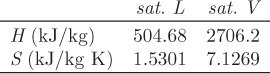
S3 = xLSL + xVSV = (1 − 0.713)(1.5301) + (0.713)(7.1269) = 5.5210 kJ/kg K.
Heat Exchanger
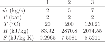
A heat exchanger is a device used to transfer heat from one fluid to another. The basic idea is simple: two fluids come into thermal contact via a conducting wall that allows heat to pass from the hotter to the cooler fluid. In this arrangement, the fluids do not intimately mix. Typically, one fluid flows inside a pipe and the other in a shell around that pipe. This design is called a shell-and-tube heat exchanger. Usually a large number of tubes are bundled together to increase the contact area and the rate of heat transfer. In terms of direction of flow, heat exchangers are classified as co- or countercurrent (Figure 6-6). In cocurrent arrangement both fluids flow in the same direction. The temperature gradient is highest at the inlet and smallest at the outlet. Given a large enough exchanger, the fluids would exit at a common temperature, corresponding to thermal equilibrium. This is not the case in practice because it would require a prohibitively large heat exchanger. In countercurrent arrangement the fluids flow in opposite directions and in this case the temperature difference between the fluids along the length of the heat exchanger is more uniform. A large variety of heat exchanger designs are covered in courses on heat transfer. For the purposes of overall energy and entropy balance, however, these design details are not important, as we will see below. Regardless of design, the driving force for the transfer of heat is the temperature difference between the two fluids at the inlet. A minimum temperature difference is required in order to accomplish the transfer at a practical rate. For our calculations we will assume as a rule of thumb a temperature difference of at least 5 °C between the temperature of the hot and cold streams.
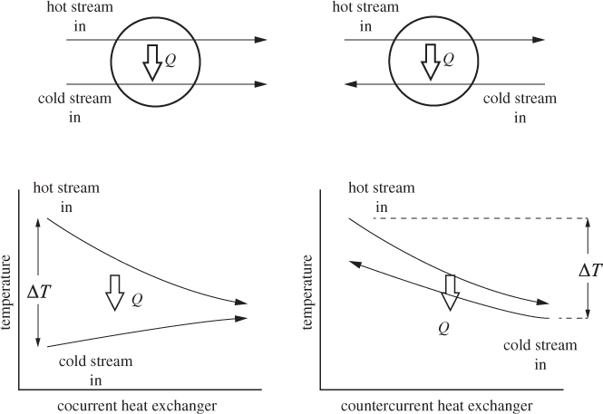
Figure 6-6: Cocurrent and countercurrent heat exchanger and their qualitative temperature profiles.
To analyze the energy transfer in the heat exchanger we take one of the streams to be the system and make the following assumptions: (a) flow is steady state; (b) kinetic and potential energy terms can be neglected; and (c) there are no heat losses to the surroundings, i.e., all heat that leaves the hot fluid is absorbed by the colder fluid. We suppose the flow rate of the inlet stream to be ![]() , and since we have steady state, this is also the same at the outlet. We will neglect variations in elevation (Δz12 = 0). Moreover, unless the diameter of the pipe changes between inlet and outlet, the velocity must be the same (
, and since we have steady state, this is also the same at the outlet. We will neglect variations in elevation (Δz12 = 0). Moreover, unless the diameter of the pipe changes between inlet and outlet, the velocity must be the same (![]() ). Finally, we set Ws equal to zero because no work is exchanged. With these assumptions, the steady-state energy balance is
). Finally, we set Ws equal to zero because no work is exchanged. With these assumptions, the steady-state energy balance is
Dividing both sides by ![]() we obtain the energy balance on a per-mass basis:
we obtain the energy balance on a per-mass basis:
The corresponding entropy balance is obtained from eq. (6.28). Dividing by ![]() we obtain the balance per unit mass of the fluid:
we obtain the balance per unit mass of the fluid:
where Tbath is the bath with which the system exchanges heat.
Q = ΔH12 = (2776.6 − 3074.5) kJ/kg = −297.9 kJ/kg.
Q = − 297.9 kJ/kg.
where ![]() ′ is the mass flow rate of cold water. We obtain
′ is the mass flow rate of cold water. We obtain ![]() ′ in terms of
′ in terms of ![]() through the energy balance. Noting that the sign of the heat must be reversed, the energy balance for the cold-water stream reads
through the energy balance. Noting that the sign of the heat must be reversed, the energy balance for the cold-water stream reads

Steam Turbine
A turbine is a device that extracts shaft work from a fluid. In its most basic form it is a fan that rotates under the action of the fluid, such as in water mills and wind mills, which have been in use for many centuries. Industrial gas turbines operate with a hot, pressurized gas, such as steam. Pressurized liquids can also be expanded to produce work and in this case the device is called an expander. The technical design details are different but the thermodynamic analysis of gas turbines and liquid expanders is done in the same way. The principle of operation is straightforward: the pressurized gas is forced to flow through converging nozzles that cause the velocity to increase. The fast-moving gas impinges on blades fixed on a rotor, which extracts shaft work in the form of rotational motion. Instead of actual nozzles, modern gas turbines utilize a set of stationary blades (stator) positioned right before the moving blades (rotor). These act as nozzles to guide the fluid onto the rotating blades. To maximize the amount of work, often multiple stages of nozzles and blades are incorporated into the same unit. Because the specific volume of an expanding gas increases, the cross section of the turbine increases in the direction of the flow.
The design and internal details of the turbine are not important when considering the overall energy balance between inlet and outlet. The operation is assumed to be adiabatic and at steady state. Variations in potential energy are unimportant (δz12 = 0). Even though the velocity of the gas varies through the turbine, the change in velocity between inlet and outlet can be neglected because it represents a small contribution to the overall balance. With these assumptions, the steady-state energy balance simplifies to
where ΔH is the enthalpy change between inlet and outlet. The entropy generation is obtained from eq. (6.28) with ![]() :
:
where ΔS is the entropy change between inlet and outlet.
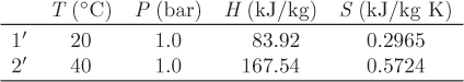
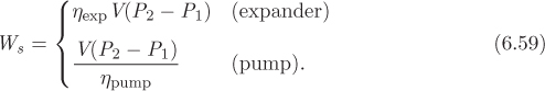
If both inlet and outlet states are known, the work is easily computed from eq. (6.46). In process design we normally know the inlet state (pressure and temperature), which is usually determined by upstream processes, and the outlet pressure, which represents a design decision. The engineer is then called to determine both the exit temperature and the work produced in the turbine. This calculation requires the efficiency of the turbine, which is defined as
where ![]() is the work for reversible expansion from the known inlet state to the known outlet pressure. This process is isentropic, since it is reversible and adiabatic. Under reversible operation the turbine produces the maximum possible work. Irreversibilities decrease the amount of work and thus the efficiency of the actual turbine is less than 100%. The efficiency of a turbine is characteristic of the device and usually available from the manufacturer. If the efficiency is known, the calculation of the turbine is done in two steps: first, we calculate the work and exit temperature for reversible operation, then we calculate the work and exit temperature for the actual operation.
is the work for reversible expansion from the known inlet state to the known outlet pressure. This process is isentropic, since it is reversible and adiabatic. Under reversible operation the turbine produces the maximum possible work. Irreversibilities decrease the amount of work and thus the efficiency of the actual turbine is less than 100%. The efficiency of a turbine is characteristic of the device and usually available from the manufacturer. If the efficiency is known, the calculation of the turbine is done in two steps: first, we calculate the work and exit temperature for reversible operation, then we calculate the work and exit temperature for the actual operation.
Reversible Operation
Let P1 and T1 refer to the inlet state and P2 to the outlet pressure. Under isentropic conditions the gas would exit at a temperature T′2 such that
This equation fixes the unknown temperature T′2. The corresponding reversible work is given by eq. (6.46):
Actual Operation
The actual work is calculated from the reversible work and the known efficiency:
The exit temperature is determined from the energy balance, eq. (6.46), which takes the form
In this equation the only unknown is T2.
The procedure is demonstrated graphically in the Mollier chart in Figure 6-7. The reversible calculation is represented by the isentropic path 12′, which on this graph is a vertical line starting at the known initial state and terminating at the known exit pressure. The actual exit state is at the same exit pressure but to the right of point 2′, corresponding to positive ΔS12 (and higher temperature than state 2′). Accordingly, the actual work, H2 − H1, is smaller than the reversible amount. The numerical details of the calculation depend on the method used for the calculation of enthalpy and entropy. This can be done using an equation of state, tabulated values, or charts. The approach will be demonstrated with examples below.
Figure 6-7: Graphical solution of turbine on Mollier graph.
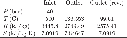
H1 = 3445.8 kJ/kg, S1 = 7.0919 kJ/kg K.
H2 = H1 + Ws = 3445.8 + (−696.31) = 2749.49 kJ/kg.
Throttling
It is often necessary to reduce the pressure of a stream before leading it to the next step of the processes. This is most easily done through a partially open valve that offers sufficient resistance to flow as to maintain the pressure difference between inlet and outlet. Clearly, there is no shaft work involved. What is the outlet temperature? To analyze this process we make a number of simplifying assumptions. First we assume there are no heat losses to the surroundings. We further assume that the velocity of the fluid that emerges at the low-pressure end of the valve is not significantly lower than the inlet velocity. Normally, a fluid moving under a large pressure difference increases its velocity (see eq. [6.39]); however, if the resistance to flow is high, the kinetic energy is dissipated into internal energy. A process that satisfies these conditions is called throttling, or Joule-Thomson expansion. The process is encountered when a pressurized fluid expands via a path of high resistance to the flow, as when a fluid passes through a partially open valve, through a porous plug, through a small crack in the walls, and the like.
To analyze this process, we apply the steady-state energy balance to a system with one inlet and one outlet, that exchanges no work or heat, and with negligible contributions from kinetic or potential energy. Under these conditions, the energy balance simplifies to
Accordingly, during throttling the enthalpy of the fluid remains constant. In typical problems we know the inlet state (pressure and temperature) and the outlet pressure. Since the outlet enthalpy is also known, pressure and enthalpy fully specify the state of the outlet.
Throttling may be viewed as expansion in a turbine that is so irreversible that no work is produced. Why should one waste the potential of a pressurized gas by throttling it rather than using a turbine to expand it? Because using a valve is much cheaper to install and maintain (no moving parts) than a turbine. Replacing a throttling valve with a turbine will increase the efficiency of a process, but the decision to replace it would have to be made on a case-by-case basis, based on cost-benefit analysis.
Sgen = S2 − S1.
Sgen ≈ 0.
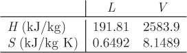
S2 = xLSL + (1 − xL)SV = (0.975)(0.6492) + (1 − 0.975)(8.1489) = 0.8357 kJ/kg K.
Sgen = S2 − S1 = 0.8357 − 0.8311 = 0.00461 kJ/kg K.
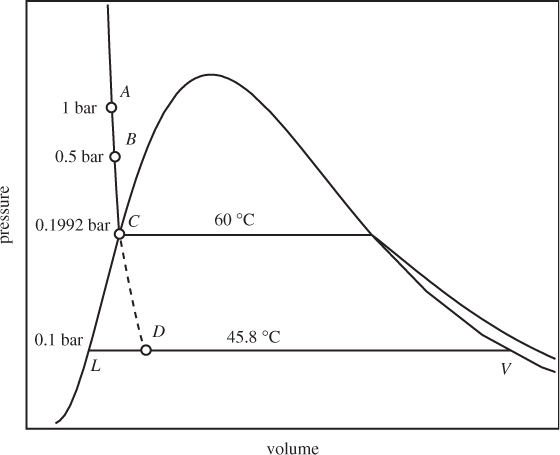
Figure 6-8: Throttling of compressed liquid (see Example 6.17).
Gas Compression
A compressor performs the opposite task of a turbine: it receives work and delivers the fluid at higher pressure. When the fluid is a liquid the device is called pump. The analysis of compressor and pumps is done on the same principles, but we will discuss each separately. There are many different designs of compressors. The axial-flow compressor is essentially a turbine working in reverse: the low pressure fluid is first accelerated by a rotating set of blades and then passes through a set of stationary blades that act as diverging nozzles and slow the flow. Multiple stages may be employed, as with turbines. Because the density of the fluid increases with pressure, the cross-sectional area of the compressor decreases in the direction of flow. Other designs use centrifugal motion, moving pistons, or helical screws to produce the compression. For the purposes of overall thermodynamic analysis, the design details are unimportant and what matters are the states of the inlet and outlet streams. We assume steady state, no heat losses to the surroundings, and negligible contribution of kinetic and potential energy terms. Under these conditions the energy balance reduces to
where ΔH is the enthalpy change between inlet and outlet. Similarly, the entropy generation is obtained from eq. (6.28) with ![]() :
:
where ΔS is the entropy change between inlet and outlet. The compressor consumes the minimum possible work under reversible operation. The actual work is higher due to irreversibilities. The efficiency of the compressor is defined as
This has the inverse form of the turbine efficiency in order to produce a number less than 100%. In the typical problem we know the inlet conditions (pressure and temperature), the outlet pressure, and the compressor efficiency. The calculation of the required work and of the exit temperature is done in complete analogy to the turbine calculation: first we compute the reversible work under the condition of isentropic operation, then we use the known efficiency to calculate the work. Finally, we calculate the enthalpy of the exit stream from the energy balance; this enthalpy and the known exit pressure are used to obtain all other properties at the outlet. These steps are demonstrated graphically on the Mollier chart in Figure 6-9.

Figure 6-9: Graphical solution of compressor on Mollier graph.
T1 = 99.6 C, H1 = 2675.4 kJ/kg, S1 = 7.3598 kJ/kg K.
T2′ = 474.626 K, H2′ = 3412.28 kJ/kg.

H2 = H1 + Ws = (2675.4) + (983.2) = 3658.07 kJ/kg.
T2 = 585.6 °C, S2 = 7.6679 kJ/kg K.
Sgen = S2 − S1 = (7.6679) − (7.3598) = 0.3091 kJ/kg K.
Expansion and Compression of Liquids
Liquids can be expanded or compressed just as gases can. For technical reasons, the design of expansion and compression units for liquids is different from that of gases, but the thermodynamics analysis is the same. A turbine for liquids is usually called an expander, and a compressor for liquids, a pump. The analysis is based on the same equations as for gases, but we treat the subject separately because the relative incompressibility of liquids allows us to use short-cut approximations for the enthalpy and entropy changes of the fluid. The starting point is eqs. (5.29) and (5.30),
which give the enthalpy and entropy in terms of the coefficient of thermal expansion, β. For both expanders and pumps, the reversible work corresponds to isentropic operation between inlet state (P1, T1) and outlet pressure (P2):
The isentropic enthalpy change is obtained from eqs. (5.29) and (5.30): we set dS = 0 in the entropy equation, solve for the term CPdT and substitute into the enthalpy equation. The result is
We integrate between inlet and outlet treating V as constant (pressure has negligible effect on the volume of liquids), to obtain
where ρ = 1/V is the density of the fluid. The actual work is calculated from the known efficiency of the device:
The enthalpy of the liquid at the exit is
H2 = H1 + Ws,
and this value, along with pressure, define the exit state. If the value of β is known, we may use eqs. (5.29) and (5.30). Alternatively, the properties at the outlet may be calculated from saturated tables by interpolation at the known enthalpy (recall that the properties of compressed liquid are to a very good approximation equal to those of the saturated liquid at the same temperature).
V1 = 0.001002 m3/kg, H1 = 83.92 kJ/kg, S1 = 0.2965 kJ/kg K.
H2 = H1 + Ws = (83.92) + (2.53) = 86.458 kJ/kg.
T2 = 20.6 °C, H2 = 86.458 kJ/kg, S2 = 0.3051 kJ/kg K.
Sgen = 0.3051 – 0.2965 = 0.0086 kJ/kg K.
6.7 Power Generation
Most industrial power generation is based on the ability of a compressed gas, often steam, to produce work through expansion in a turbine. Water from ambient conditions (a river or lake) is compressed and boiled to produce high-pressure steam, which expands in a turbine. The exhausted steam is recycled to the process to form a continuous closed loop. The basic process diagram of the power plant is shown in Figure 6-10. Here, in addition to the pump, boiler and turbine, we also encounter a condenser, which cools and condenses the exhausted steam before it is pumped again into the boiler. To see why the condenser is necessary, we examine the operation of the plant on the TS graph in Figure 6-11 (the compressed liquid region is exaggerated on this graph; in reality, lines of constant pressure lie very close to the line of saturated liquid). We trace the path of the process by starting at the pump, which compresses the liquid (state 4) to higher pressure (state 1), For isentropic compression the path on the TS graph is a vertical line moving up; if the pump efficiency is less than 100%, the actual path veers to the right, as it results in positive entropy change. The pressurized liquid is heated in the boiler to produce superheated steam (state 2), which then passes through the turbine. The exhausted stream is superheated vapor at lower pressure (condensation is to be avoided in the turbine). Since the efficiency of real turbines is less than 100%, the expansion follows a path to the right of the isentropic path, shown by a vertical dashed line. To return this stream, which is still hot, back to the pump, it must be cooled and condensed. Why not cool the exhausted steam by additional expansions? In fact, steam is usually expanded in multiple stages to maximize the amount of work. However, expansion cannot move the state to the left, toward state 4. In fact, reversible expansion can only move the state vertically down (isentropic expansion), while irreversibilities cause the state to move to the right (corresponding to positive ΔS). A condenser is indeed necessary and shows in practice that it is not possible to convert the entire amount of heat that enters the boiler into work.
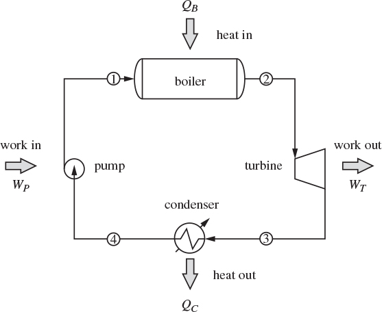
Figure 6-10: Rankine power plant.
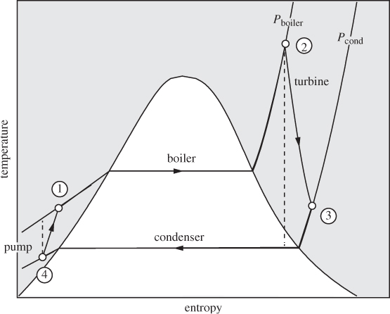
Figure 6-11: Rankine power plant on the TS graph. Dashed lines correspond to isentropic operation in the pump and turbine.
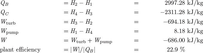
The process shown in Figures 6-10 and 6-11 is called a Rankine plant and in its basic form, shown here, operates between two pressures, a high pressure at the inlet of the turbine, and a low pressure at the exit. Ignoring pressure drop through pipes, the boiler, and the condenser, streams 1 and 2 are at the high pressure, while streams 3 and 4 are at the low pressure. In terms of energy inputs and outputs, the cycle absorbs heat in the boiler to produce work in the turbine. Part of the input heat is rejected in the condenser. A small amount of work is also consumed in the pump. The overall balance is5
5. The energy terms in this balance are expressed per unit mass of the fluid. Alternatively, they can be expressed per unit time by multiplying the above values by the mass flow rate.
where we understand QB and WP to be positive, and QC and WT to be negative. The net amount of work produced is
Since the amount of pumping work is much smaller than the work received in the turbine (see Example 6.19), there is a net production of work. The efficiency of the plant is defined as the ratio of the net work produced to the amount of heat in the boiler:
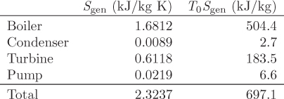
This efficiency is limited by the second law: if the heat source that provides heat to the boiler is at TB and the condenser rejects heat to a reservoir at TC, the steady-state entropy balance gives6
6. Start with the steady-state entropy balance, eq. (6.28), set Δ(![]() S) to zero because the fluid operates in a cycle, and note that the plant exchanges heat with two baths.
S) to zero because the fluid operates in a cycle, and note that the plant exchanges heat with two baths.
Eliminating QC between eqs. (6.60) and (6.63) and solving for the ratio −W/QB, which is equal to the plant efficiency, we obtain
Since both Sgen and QB are positive terms we must have,
which states that the efficiency of the plant is limited by the maximum Carnot efficiency that corresponds to the temperatures of the two heat baths. Temperature TB corresponds to the temperature of the heat sources (for example, the flame temperature of coal combustion, if this is a coal-fired plant) and must be at least equal to the temperature of stream 2, which is the hottest stream in the process. Temperature TC may be taken to be the same as T4 (the coldest temperature in the plant), or equal to the temperature of the surroundings, since the cooling medium is usually ambient water or air.7
7. In cooling towers, often seen in large power plants, the cooling is provided by the atmosphere.
Wrev = − 925.579 kJ/kg.
H3 = H2 + η Wrev = 2728.72 kJ/kg.
T3 = 126.2 °C, S3 = 7.4942 kJ/kg K.
H1 = H4 + Wpump = 425.621 kJ/kg.
T1 = 101.5 °C, S1 = 1.3245 kJ/kg K.

6.8 Refrigeration
To achieve temperatures below ambient we must use some type of refrigeration. In general, this requires work in order to maintain a temperature gradient between the desired low temperature and that of the surroundings. A common design is based on a familiar principle: if we are wet and sit by a breeze, it feels cool. This is because evaporation requires heat and this is drawn from our body, causing the temperature to drop. The breeze accelerates the evaporation rate by removing vapors from the immediate vicinity of the liquid, thus intensifying the cool feeling of coolness. However, it is the evaporation, not the breeze, that is responsible for the main effect. This situation can be replicated experimentally by expanding a liquid into the vapor-liquid region. As we saw in Example 6.17, if a compressed liquid is throttled (or expanded through a turbine) into the two-phase region, the temperature drops to the saturation temperature that corresponds to the pressure of the expanded liquid. Accordingly, the temperature is controlled by the pressure of the expanded liquid. This phenomenon forms the principle of operation of most refrigeration processes, from household refrigerators and to air-conditioning units, to industrial cryogenic processes. The basic vapor compression cycle is shown in Figure 6-12. Compressed liquid (stream 1) is throttled to lower pressure such that the state at the exit of the valve is a vapor-liquid mixture (state 2). This cold stream passes through a heat exchanger in which the vapor-liquid mixture evaporates by drawing heat from the warm stream that is to be cooled. The refrigerant exits the evaporator as saturated vapor (stream 3). To return to throttling, the vapor must be compressed. The state at the exit of the compressor is superheated vapor (state 4). To regenerate the compressed liquid, the vapor is condensed in a heat exchanger (condenser), which completes the cycle. In terms of energy exchanges, the cycle absorbs heat in the evaporator, consumes work in the compressor, and rejects heat in the condenser. The net effect is to “pump” heat from the low temperature of the evaporator to the higher temperature in the condenser through the input of work. This cycle is essentially the reverse of the Rankine power plant. The throttling valve may be replaced by an expander; this would accomplish the expansion while also producing some work, which could be used towards the compression. Most units utilize a throttling valve instead because it is much simpler to operate and maintain, but also because the amount of work that can be extracted from the expansion of a liquid is rather small.
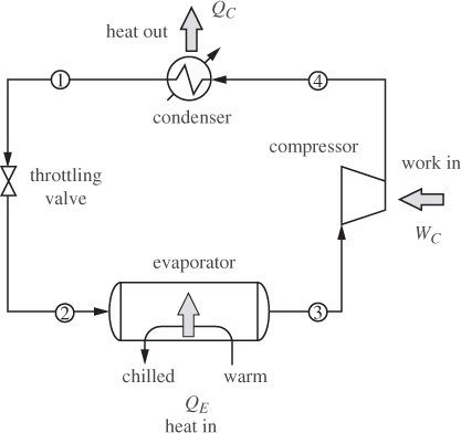
Figure 6-12: Vapor-compression refrigeration cycle.
Refrigeration cycles are often represented on the PH chart, which may also be used to perform a graphical solution of the energy balances. Figure 6-13 shows the path of the vapor compression cycle on this chart. Ignoring pressure drops in pipes and heat exchangers, the cycle operates between two pressures, a high pressure that is achieved by the compressor, and a lower pressure that is accomplished by throttling. On the PH chart throttling is represented by a vertical line at constant enthalpy. Heat transfer in the evaporator and in the condenser takes place at constant pressure. For a reversible compressor, the path would follow a line of constant entropy; for a real compressor with an efficiency less than 100%, the compressed vapor emerges hotter and to the right of the isentropic path. The temperature of the evaporator is controlled by the throttling pressure. The lower this pressure, the colder the temperature. It is generally desirable, however, to maintain the pressure in the evaporator near or above atmospheric in order to avoid the expense of vacuum equipment.
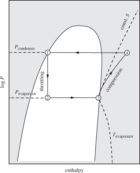
Figure 6-13: Refrigeration cycle on the PH graph.
Thermodynamic Analysis of Refrigeration
The energy balance on the refrigeration cycle is
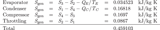
where QE is the amount of heat removed from the evaporator (QE > 0), QC is the amount of heat rejected in the condenser (QC < 0), and WC is the work for compression (WC > 0). The entropy balance is obtained by noting that the refrigerant operates as a cycle and thus does not contribute to the generation of entropy.
Treating the evaporator and the condenser as baths at temperatures TE and TC, respectively, the entropy generation is
The performance of refrigeration cycles is assessed via the coefficient of performance (cop), which is defined as the amount of heat extracted in the evaporator over the amount of work in the compressor:
This ratio represents the refrigeration capacity over the refrigeration “cost” in terms of work. Unlike the efficiency of the power plant, the coefficient of performance is not restricted to be less than one. Its maximum value is, however, limited by the second law. To determine the limiting value of the coefficient of performance, we solve the entropy balance for QC, substitute into the energy balance and solve the resulting equation for the ratio QE/W; we find:
The quantity (SgenTCTE)/QE in the denominator is positive, which implies that entropy generation decreases the coefficient of performance. The maximum value of the coefficient of performance is obtained under reversible operation. Setting Sgen = 0 we find
This is the maximum coefficient of performance and corresponds to a Carnot refrigerator that operates reversibly between temperatures TE and TC.
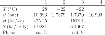
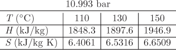
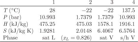
T4′ = 110.096 C, P4 = 10.993 bar, H4′ = 1848.54 kJ/kg, S4′ = 6.4067 kJ/kg K.
Wrev = 1848.54 − 1578.1 = 270.436 kJ/kg,
S2 = (0.826)(1.0896) + (1 − 0.826)(6.4067) = 2.0148 kJ/kg K.

Refrigerants
Refrigerants are classified by a code of the form RXYZ, where XYZ is a unique number assigned to the fluid. These codes are assigned by the American Society of Heating, Refrigerating and Air-Conditioning Engineers (ASHRAE). Water, for example is given the refrigerant code R718. Some common refrigerants are given in Table 6-1.8 In principle any fluid can be used as refrigerant in a vapor compression cycle, however, some physical and practical limitations apply. For example, water freezes at 0 °C, therefore it cannot be used in subfreezing temperatures. Other limitations are imposed by practical operating constraints. It is generally desirable to operate at pressures above ambient. Lower pressures require vacuum equipment, which is more expensive. A second consideration is with respect to the operation of the condenser. The temperature at the compressor exit must be at least 20 °C or so to allow the use of ambient water or air as the coolant. This temperature determines the saturation pressure in the condenser and the minimum pressure that must be achieved by compression. The saturation pressures in the evaporator and condenser set the pressures of the cycle and the demand of the compressor. For this reason, the saturation pressure is the most important property of the fluid with respect to refrigeration.
8. For an explanation of the naming algorithm see www.epa.gov/ozone/geninfo/numbers.html.
Table 6-1: Some common refrigerants and their ASHRAE designation.
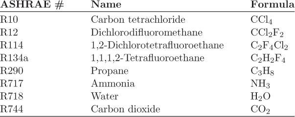
Figure 6-14 shows the saturation pressure of some common refrigerants. If we are designing a refrigeration cycle with an evaporator at −20 °C, we could select ammonia, R12 or R134, which are very similar to each other. This would place the evaporator pressure at about 1 bar and the condenser at about 10 bar, requiring a compression ratio of 10:1. Ethane, on the other hand, would not be appropriate because it would require operation between ~ 10 and 60 bar, a considerably higher pressure. If the evaporator requires much lower temperatures, say, −100 °C, ethane (normal boiling point about −89 °C) would be a good candidate. This cycle would require a pressure of about 0.5 bar in the evaporator but at least 40 bar in the condenser. If the condenser is operated at lower pressure, condensation will require refrigeration. This is often more desirable than operating a single stage up to a very high pressure. This cascade design then, uses two refrigerators, one to produce the required low temperature, and another to condense the compressed vapor of the low-temperature refrigerant.

Figure 6-14: Saturation pressure of some common refrigerants.
Note
Refrigerants and the Environment
An important consideration in choosing the refrigerant is chemical toxicity. Chlorofluorocarbons, or CFCs, have the general chemical formula CnFmCl2n+2−m and are remarkably inert. These fluids were developed after World War II and found widespread use as refrigerants (known under the trade name Freon), but also as fire retardants and as propellants in household spray cans. An unintended consequence of their inert nature is that they do not decompose easily and have long lifetimes in the atmosphere, where they participate in reactions that deplete the ozone in the stratosphere. Since the late 70s their use is being phased out. Their replacements are molecules that are not fully halogenated but contain some hydrogen. One such molecule is tetrafluoroethane, also known as HFC-134a. The ozone impact of gases is reported as its ozone depletion potential (ODP), which measures the chemical effect of the molecule relative to that of trichlorofluoromethane (R11). Another property is the global warming potential (GWP), which characterizes the impact of the gas on global warming relative to that of carbon dioxide. For a list of ODP and GWP factors of various refrigerants, see www.epa.gov/ozone/science/ods/index.html.
6.9 Liquefaction
One application of refrigeration is in the liquefaction of air, nitrogen, and other gases that under ambient conditions are above their critical temperature. There are several industrial applications for liquefied gases. The separation of air into its components by distillation is the basis for the industrial production of inert gases such as nitrogen, argon, and helium. Liquid oxygen is used as a rocket fuel; natural gas (mostly methane) is liquefied for the purposes of increasing its density for transportation and storage purposes; liquid nitrogen provides a convenient heat bath for low temperature experiments. To appreciate the magnitude of the refrigeration problem, consider the liquefaction of nitrogen. Figure 6-15 shows the qualitative PH graph of nitrogen. At ambient conditions (state A) nitrogen is a gas above its critical temperature (−144 °C). To produce liquid nitrogen at 1 bar, the temperature must be lowered to −196 °C, its normal boiling point. The system can be brought into the two-phase region by throttling from a high pressure (state D). To produce such state, the nitrogen must be compressed (state B) and then cooled under constant pressure. Part of the required cooling can be done with water, but this will only cool the hot vapor to about 25 °C (state C). Further cooling to state D requires refrigeration. This may be provided by the cold vapor that is produced at the exit of the throttling valve.
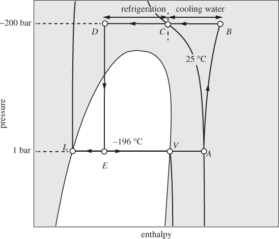
Figure 6-15: Illustration of the liquefaction of nitrogen on the PH graph (not to scale).
A process that accomplishes these steps is shown in Figure 6-16. Liquid nitrogen is produced by throttling the compressed stream 5 to 1 bar (stream 6). The liquid fraction (stream 7) is collected as the product, and the vapor (stream 8) is used to chill the compressed nitrogen vapor, after it has been cooled to room temperature by a precooler using ambient water. This vapor is then mixed with the fresh nitrogen stream and is recycled through the process. This is known as the Linde liquefaction process. There is no external refrigeration, instead, nitrogen acts as its own refrigerant. For this process to work, the compressor pressure must be fairly high so that the precooler can accomplish a significant part of the cooling. If not, as more of the heat load is shifted from the precooler to the cooler, the process reaches a point where it does not produce enough cold vapor to sustain the required temperature of stream 5.
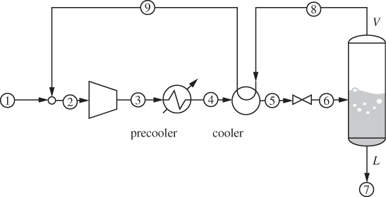
Figure 6-16: Linde process for gas liquefaction.
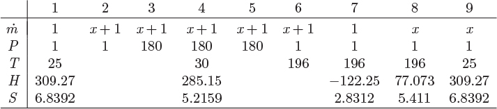
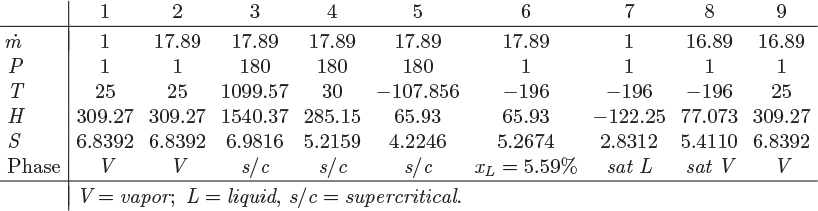
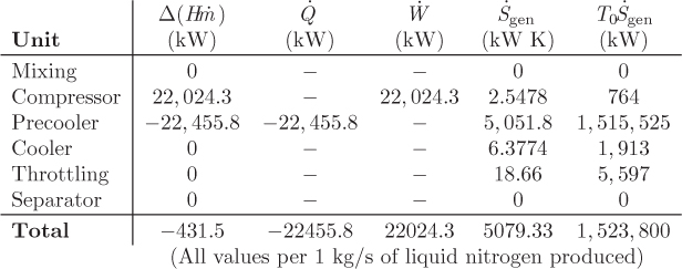
Here, ![]() is the mass flow rate in stream 8 on the basis of 1 kg of liquid nitrogen, P is in bar, T is in °C, H is kJ/kg, and S is kJ/kg K.
is the mass flow rate in stream 8 on the basis of 1 kg of liquid nitrogen, P is in bar, T is in °C, H is kJ/kg, and S is kJ/kg K.
H6 = xLHL + xVHV = (0.0559)(−122.25) + (0.9441)(77.073) = 65.9314 kJ/kg
S6 = xLSL + xVSV = (0.0559)(2.8312) + (0.9441)(5.4116) = 5.26736 kJ/kg K.
H5 = H6 = 65.9314 kJ/kg.
T5 = − 107.9 °C, S5 = 4.2246 kJ/kg K.
Qcooler = |m9H9 − m8H8| = |m5H5 − m4H4| = 3921.81 kW.
where ![]() is the amount of heat exchanged with an external heat bath and T is the temperature of that bath. Only the precooler exchanges heat with the surroundings (cooling water). Taking the temperature of cooling water to be 25 °C we set Tbath = 298.15 K.
is the amount of heat exchanged with an external heat bath and T is the temperature of that bath. Only the precooler exchanges heat with the surroundings (cooling water). Taking the temperature of cooling water to be 25 °C we set Tbath = 298.15 K.
• For every kg of liquid nitrogen produced, 16.89 kg of nitrogen must circulate through the system in a closed loop. This flow acts as the refrigerant: it is compressed, cooled, and throttled, as in usual refrigeration cycles. The only difference is that instead of using a standard evaporator to cool the incoming stream, it is directly mixed with it.
• The large recirculation flow also means the liquid fraction in stream 6 is small, only 5.6%. In this respect, the situation is somewhat different from that in Figure 6-15 in that state E (corresponding to stream 6) is much closer to state V that this figure shows. In other words, the process barely brings the state of the throttled fluid into the two-phase region. Producing more liquid would require further cooling in the cooler, and higher pressure in the compressor.
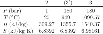
• The compression ratio (180:1) is large and the temperature at the exit of the compressor high (1100 °C). The compression should be done in stages so that each compression involves a smaller compression ratio with intercooling between stages.
• In terms of entropy production, by far the main contribution comes from the precooler. This amount was calculated assuming the cooling water to be at 25 °C. If this stream is specified in terms of flow rate, its contribution to the entropy generation would be calculated by replacing the bath term with ![]() cwΔScw, where
cwΔScw, where ![]() cw is the flow rate of this stream and ΔScw is its entropy change through the heat exchanger.
cw is the flow rate of this stream and ΔScw is its entropy change through the heat exchanger.
• Streams are always mixed at the same pressure to avoid backflows. This process is generally irreversible and results in entropy generation as the mixed streams are usually at different temperatures. In the above process, it is a lucky coincidence that streams 1 and 9 are mixed at same temperature. In this, special case mixing is a reversible process and results in no entropy production.
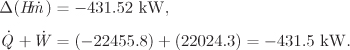
• It is generally a very good practice to include in the summary table the calculation of Δ(![]() ) for every unit and confirm that the energy balance is satisfied for all units. For example, the energy balance in the precooler was not used in the calculation because it is redundant with the other balances used. One must confirm, however, that the balance is indeed satisfied. This acts as a check of the calculation. As a further check, one should confirm the overall energy balance:
) for every unit and confirm that the energy balance is satisfied for all units. For example, the energy balance in the precooler was not used in the calculation because it is redundant with the other balances used. One must confirm, however, that the balance is indeed satisfied. This acts as a check of the calculation. As a further check, one should confirm the overall energy balance:
Note
On the Thermodynamic Analysis of Processes
The overall lesson from Example 6.23 is that flow sheets of moderate complexity, with several units and recycle streams, can be solved by hand in a systematic way, as long as the properties of the fluid are known, either from tables or from software applications. The calculation is always reduced to the energy balance around an individual unit, such as a compressor, a throttling valve, and the like. For relatively simple flow sheets, one will normally use the energy balance to calculate one unknown stream, then move serially to the next unknown stream and continue until all streams are known. With more complex flow sheets, such as the one here, several units may have to be solved simultaneously to obtain the unknown properties. For example, the separator, throttling valve, and precooler involve common unknown streams and cannot be solved as individual units. By combining such units to write an overall balance for the whole group it is sometimes possible to eliminate the intermediate unknowns. Otherwise, multiple units will have to be solved simultaneously. Once the streams are known, the energy and entropy balances are computed easily. Assumptions about baths need to be made only if a process stream exchanges heat with an unspecified stream. Though the main interest is in the energy balances, the entropy balance also provides very useful information for the sources of irreversibility. An efficient process should minimize entropy production because this leads to savings in terms of better energy utilization. Process design is beyond the scope of this book, but what should be clear is that the entropy analysis of a process is the starting point for optimizing the overall efficiency of the process.
6.10 Unsteady-State Balances
While the majority of processes encountered in plants are open processes running at steady state, there are also situations that involve unsteady-state operation. The analysis proceeds by the same general methodology as with steady-state, except that the accumulation terms are retained. However, unsteady state processes require special attention because some of the results obtained previously under steady state cannot be transferred automatically to unsteady-state processes. We examine below some typical examples of unsteady-state analysis.
Pressurizing a Tank
We consider the problem of filling a tank from a pressurized line, as shown in Figure 6-17. A main line carries the fluid at fixed pressure and temperature. A stream is drawn from this line and passes through a valve into a tank. The tank is initially at a pressure lower than that of stream 1 and it may be fully evacuated, or partially filled. As fluid fills the tank, the pressure in the tank increases until it reaches the pressure of the supply line. The valve can be closed at any point, to produce a partially filled tank. We want to find the amount (mass) of fluid and its temperature at any point during filling. We will neglect kinetic and potential energy contributions. We will also assume that the process is adiabatic. If not, additional information must be given about possible heat exchange with the surroundings. We note, however, that heat transfer is generally much slower than mass flow, therefore, even if the tank is not insulated, we may still assume that any temperature change resulting from the expansion of the gas through the valve will resist equilibration with the surroundings over the duration of the process. In this respect, the process may be modeled as approximately adiabatic. To perform balances we define the system to be the tank and the valve, shown by the dashed line in Figure 6-17. We neglect the mass of the fluid in the line and in the valve and take the entire mass M of the system to be the mass of the gas inside the tank. We will further assume that pressure and temperature inside the tank is uniform. This may be a rather crude approximation, as there is definitely flow between the point where the pipe connects to the tank and the bulk of the tank. However, such details cannot be accounted for in our formulation of the energy balance, which is macroscopic. For this reason, we will have to accept this approximation. Initially the tank contains M0 mass of the fluid at T0, P0. The main line is assumed to come from a large supply tank so that the conditions of stream 1 do not change as the tank is being filled.

Figure 6-17: Pressurizing and venting of tank.
We begin with the mass balance. With one inlet flow (![]() 1) and no outlet, eq. (6.8) becomes
1) and no outlet, eq. (6.8) becomes
Multiplying both sides by dt this becomes
The last result simply states that the increase of the mass in the system over time dt is equal to the amount of mass that crosses into the system during this time. The energy balance is
where Utot = MU is the total internal energy in the tank, and U is the specific or molar (depending on whether M is expressed in kg or mol) internal energy at the pressure and temperature of the tank. Multiplying by dt both sides of the energy balance we obtain
The last result states that all the enthalpy that is carried into the system is accounted for as internal energy. This equation can be integrated from initial conditions (Utot = M0U0, m1 = 0) up to the point that a total mass m has been introduced to the tank (Utot = MU, m1 = m). Noting that the mass in the tank at the final state is M0 + m and that H1 is constant, the result of this integration is
(M0 + m)U − M0U0 = H1m,
which can further be written as
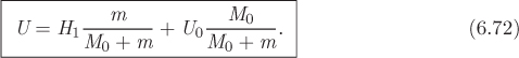
This equation specifies an intensive property in the tank (specific or molar internal energy) at the point where it has admitted an amount of mass m. An additional property must be specified to fully define the state in the tank. This will depend on the specifics of the problem. For example, if the volume Vtank of the tank is known, then the specific volume is V = Vtank/(M0 + m), and this provides the additional intensive variable for the complete specification of the state.
T1 = 250 °C, P1 = 20 bar, H1 = 2903.2 kJ/kg.
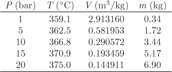
T = 366.748 °C, V = 0.290572 m3/kg.
Repeat the previous problem assuming steam to be an ideal gas with ![]() J/mol K.
J/mol K.
Venting a Tank
We consider now the opposite problem, venting a tank into the ambient surroundings. The tank contents are at pressure P and temperature T and the surroundings at P0, T0. Venting is done through a valve. Over a small time, dt, an amount of fluid, dm, leaves the tank and emerges in the surroundings. The pressure of this element at the venting point is the same as the pressure of the surroundings. Its temperature, however, is not that of the surrounding air but is determined by the process. Eventually, of course, this mass will equilibrate with the surroundings. Thermal equilibration, however, is slow and the process may be treated as adiabatics.9 We will also assume the contents of the tank to be at a uniform state, effectively ignoring the pressure gradients that cause the fluid to flow from the bulk of the tank to the entrance of the valve. Under these assumptions, the gas is throttled from the conditions in the tank (pressure P, temperature T) to pressure P0 and temperature T′ at the exit of the vent. Starting with the mass balance equation, we have
9. This is analogous to blowing air from the mouth: it comes out warm, even in a cold day, despite the fact that it is out in the open.
which says that the mass in the tank decreases by the amount withdrawn. Ignoring kinetic and potential energy effects, and setting ![]() , the energy balance is
, the energy balance is
where Utot = MU is the total internal energy in the tank, U is the specific internal energy in the tank, and H′ = H(P0, T′) is the enthalpy at the venting point. We multiply the energy balance by dt and use dm = −dM to obtain
As the tank vents, its pressure and temperature change, and so does the temperature at the exit of the vent. Accordingly, Hʹ varies with time and eq. (6.73) cannot be integrated yet until we determine how this variation is related to the state inside the tank. To establish this relationship we imagine the process to take place as follows: first an amount dm is removed from the tank; it is then throttled from pressure P, and temperature T, to the conditions at the exit of the vent. We assume now that the removal of the amount dm from the tank is done reversibly. This amounts to ignoring any pressure gradients and viscous effects in the flow of that mass from the bulk of the tank to the entrance of the valve. By removing the mass dm from the tank, the state in the tank will change. The corresponding entropy balance following this change is
where S is the specific entropy in the tank, also equal to the specific entropy carried away by the mass dm, and ![]() is the entropy generation for the removal of mass dm, which we have assumed to be zero. Expanding the differential in the right-hand side of the above equation we have
is the entropy generation for the removal of mass dm, which we have assumed to be zero. Expanding the differential in the right-hand side of the above equation we have
MdS + SdM + Sdm = 0,
and using dm = −dM, this becomes
The result states that the specific entropy in the tank remains constant at all times; it is, therefore, equal to its value at the beginning of the venting process. This provides the additional equation for the integration of the energy balance equation. We return to eq. (6.73) and work on the derivative d(MU)/dM. First, we note that this derivative expresses changes in the tank that occur at constant specific entropy. Using M = Vtank/V, where Vtank is the tank volume and V is the specific volume in the tank, we obtain a very simple result that derivative:
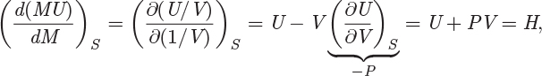
where we used eq. (5.12) to recognize the partial derivative (∂U/∂V)S as the pressure in the tank. Finally, combining this result with eq. (6.73), we obtain the desired relationship between H′ and the state in the tank:
which states that the enthalpy of the vented fluid is equal to the enthalpy in the tank at the same moment. This, along with the isentropic condition in eq. (6.74), form two equations that fully define the process:
where (P, T) is the state in the tank and (P0, T′) is the state at the exit of the vent. One may wonder why we took such a circuitous path to arrive at eq. (6.75), which, after all, expresses the familiar result that throttling is isenthalpic. One reason is that, as we saw in the problem of pressurizing a tank, under unsteady-state conditions we do not always obtain the familiar results of steady-state analysis. Moreover, the isenthalpic condition is not enough to solve this problem, we need the isentropic condition as well. Our approach shows that the assumption of reversibility in the tank leads to both conditions. And by laying out the assumptions of the calculation, we know exactly under what circumstances we may expect the solution to apply in a real situation.
Note
Pressurizing and Venting
Although venting is the reverse of pressurization, we have obtained quite different results for the two cases. The reason is that these processes are irreversible: the path for venting is not the same as the reverse of the pressurization path.


T′ = 265.3 °C.
Repeat the previous problem assuming steam to be an ideal gas with ![]() J/mol K.
J/mol K.

T′ = T = 281.8 °C.
6.11 Summary
The mathematical form of the first and second law is different for open and for closed systems. In a closed system these equations are:
where W is the PV and shaft work combined, and Δ refers to the difference between before and after. In an open system with flow streams the corresponding equations are:
Here, Ws is the shaft work only and Δ refers to the sum of all outlet streams minus the sum of all inlets. The most significant difference is that the thermodynamic property that appears inside the operator Δ is internal energy, if the system is closed, but enthalpy, if the system is open. Because the equations are different, it is important to correctly identify the system as open or closed before applying the energy and entropy balances.
With respect to open systems, we make the additional distinction between steady-state, and unsteady-state operation. At steady state the accumulation terms, dUtot/dt, dStot/dt and dMtot/dt, are zero. This reduces the energy balance from a differential equation into an algebraic equation. For this reason, steady-state processes are much simpler to calculate compared to unsteady-state processes.
Even the most complex process consists of simple units interconnected through streams. The simple units we encountered in this chapter encountered heat exchangers, pumps, compressors, turbines, throttling valves, vapor/liquid separators, and mixing points. Other common units in chemical plants are distillation columns, absorption towers, and chemical reactors. These are also analyzed by the general tools of the thermodynamics; however, they involve mixtures of multiple components, and we will postpone their discussion until we develop methods for the calculation of mixture properties.
The general strategy in working with flow sheets of low to moderate complexity is to break them down into smaller parts and apply the energy balance to one simple unit at a time with the goal to calculate the properties of all streams. Remember that if we know any two intensive properties of a stream, all other intensive properties are fixed. It is generally the practice to neglect pressure drops due to flow, at least at the preliminary stage of design. This means that the pressure in consecutive streams is taken to be the same unless the fluid passes through pumps, compressors, turbines, expanders, or throttling valves, units that are meant to change pressure. The energy and entropy balances are computed very easily once the streams are known. The purpose of the energy balance is, of course, to determine the shaft work and heat load requirements of the process. The entropy balance serves as a diagnostic tool to assess the overall efficiency of the process. By multiplying the entropy generation by a characteristic temperature T0, which we take to be that of the surroundings, we translate the irreversible features of a process into units of work. This represents the amount of work that would be gained if the underlying irreversibility were eliminated. It is not possible, nor desirable, to eliminate all irreversible features. A certain magnitude of gradients is necessary to produce practical rates in the operation of a process. However, entropy analysis provides us with a way to compare alternative designs, uncover design flaws, and optimize the overall efficiency of the process so that it makes better utilization of the available resources.
6.12 Problems
Problem 6.1: A flow process produces work using water as the working medium. The process is as follows: steam of quality 50% at 1 bar is compressed adiabatically to 20 bar; is heated isothermally by absorbing 3500 kJ/kg of heat; is expanded adiabatically to an unspecified final pressure; and is finally cooled isothermally until the steam returns to its initial state (steam of quality 50% at 1 bar). It is further reported that 53% of the heat added during the heating step is rejected during the cooling step. What is your evaluation of this process?
Problem 6.2: The power generation unit in your plant uses a hot exhaust gas from another process to produce work. The gas enters at 10 bar and 350 °C and exits at 1 bar and 40 °C. The process produces a net amount of work equal to 4,500 J/mol and it exchanges an unknown amount of heat with the surroundings.
a) Determine the amount of heat exchanged with the surroundings. Is this heat absorbed or rejected by the system?
b) Calculate the entropy change of the exhaust gas.
c) As a young and ambitious engineer you seek ways to improve the process. What is the maximum amount of work that you could extract from this system? Assume that the inlet and outlet conditions of the exhaust gas remain the same.
Additional data: Assume the surroundings to be at the constant temperature of 25 °C and the exhaust gas to be ideal with CP = 29.3 J/mol K.
Problem 6.3: You are responsible for a high-temperature process that produces two exhaust streams, stream A at 600 °C, 10 bar, with molar flow rate 100 mole/s; and stream B at 200 °C, 20 bar, with molar flow rate 50 mole/s. A young engineer in your team comes to you with an idea to utilize these streams to produce heat and work which will save costs in your process. She quickly puts together a sketch for a process that produces 220 kW of heat, 1700 kW of work, and delivers the exhaust gases as a single stream at 1 bar. The heat will be used to produce saturated steam at 1 atm by boiling the saturated liquid.
a) What is the temperature of the exit stream?
b) Should you take this idea to your superiors for further discussions?
c) Could you use the heat from this process to boil water at 10 bar?
Additional information: Assume the exhaust gases can be treated as an ideal gas with CP = 30 J/mole K.
Problem 6.4: You are in charge of a unit that produces two streams, A at 600 °C, 10 bar, with molar flow rate 100 mole/s; and B at 200 °C, 20 bar, with molar flow rate 50 mole/s. Those streams are currently throttled to 1 bar. An engineer in your team comes to you with an idea to utilize these streams to produce heat and work. She believes she can extract 1700 kW of work and 500 kW of heat that will be used to boil water at 1 bar. Her process, whose details are yet to be determined, will receive streams A and B as inlet and will have a single outlet stream that will be delivered at 1 bar.
a) What is the temperature of the exit stream?
b) Should you take this idea to your manager for further discussions?
c) Could you use the heat from this process to boil water at 10 bar?
Additional information: Assume the exhaust gases can be treated as an ideal gas with CP = 30 J/mole K.
Problem 6.5: Liquid propane boils in a constant pressure boiler to produce propane vapor at 30 bar and 245 °C. At the inlet of the boiler the propane is saturated liquid.
a) Draw a PV graph and show this process. Show all the relevant temperatures and pressures as well as the critical isotherm and the critical pressure.
b) Calculate the entropy change of propane between the inlet and outlet of the boiler. Explain your calculations and procedure clearly.
Additional data
The saturation temperature at 30 bar is 78 °C.
The heat of vaporization at 78 °C is 8780 J/mol.
The ideal-gas CP of propane vapor is 112 J/mol K.
Problem 6.6: Steam flows in a long, noninsulated pipe under a constant pressure of 2 bar. At the inlet of the pipe the temperature is 300 °C. Due to losses to the surroundings, the temperature at the exit of the pipe is 60 °C. Assume the surroundings to be at 25 °C.
a) Draw a PV graph for the steam. Show the path of the process and all the relevant pressures and isotherms.
b) Calculate the amount of heat removed from the steam.
c) Calculate the entropy change of the steam.
d) Calculate the entropy change of the surroundings. What is the entropy generation?
Problem 6.7: Steam at 5 bar, 300 °C is condensed to saturated liquid at 5 bar in a heat exchanger at a mass flow rate of 1 kg/s. Cooling is provided by water, which enters the heat exchanger at 20 °C 1 bar and exits at 60 °C. Neglecting pressure drop in pipes and heat losses to the surroundings, determine the flow rate of the cooling water, the amount of heat that is exchanged, and the rate of entropy generation.
Problem 6.8: Steam enters a cooling tower at 200 °C and exits at 60 °C. Cooling is supplied by the surroundings which are assumed to be at 30 °C. The process takes place under atmospheric pressure (1 bar).
a) Calculate the amount of heat removed from the steam.
b) Calculate the entropy change of the steam.
c) What is the entropy generation?
d) Draw a PV graph and show the path of this process.
Problem 6.9: Water at 1 bar, 20 °C is heated in a heat exchanger to produce saturated steam. The heat is provided by a stream of saturated steam at 10 bar that exits the heat exchanger as saturated liquid.
a) Calculate the amount of heat that is exchanged between the two streams.
b) Calculate the mass flow rate of the 10 bar stream.
c) Calculate the entropy generation.
Report the results per kg of liquid water entering the heat exchanger.
Problem 6.10: Stream 1 enters a tank carrying steam at 5 bar, 300 °C at the rate of 1 kg/s. The stream is cooled by adiabatic mixing with water at 5 bar, 40 °C (stream 2). If the resulting stream is a vapor-liquid mixture with quality 18%, calculate the mass flow rate of stream 2, the entropy generation, and the lost work.
Problem 6.11: A steam turbine generates power by expanding steam from 30 bar, 450 °C to 8 bar.
a) Determine the amount of work and the exit temperature if operation is reversible.
b) Repeat the calculation assuming an efficiency of 80%. How much is the lost work due to the reduced efficiency?
Problem 6.12: A thermally insulated turbine generates 750 kW of power by expanding steam from 500 C and 3.5 MPa to 200 C and 0.3 MPa.
a) What is the mass flow rate of steam through the turbine?
b) Because of failure in the insulation there is a loss of 60 kJ per kg of steam. What is the power produced by the turbine if all inlet and outlet conditions remain the same?
Assume negligible kinetic and potential energy changes.
Problem 6.13: Steam at 500 C and 40 bar passes through two turbines arranged in parallel, and their exit streams are combined into one stream. Turbine 1 has 100% efficiency, while the efficiency of turbine 2 is 75%. Both turbines exhaust at 1 bar. The stream that is formed by combining the exhausts of the two turbines is saturated vapor.
a) Determine the fraction of the total flow rate that passes through each turbine.
b) Determine the rate of entropy generation. What are the irreversible feature of this process?
Problem 6.14: A steam turbine generates 800 kW of work by expanding steam from 50 bar, 400 °C to 1 bar. At the exit of the turbine the steam contains 2% moisture.
a) Determine the flow rate of steam through the turbine.
b) Determine the efficiency.
c) Determine the rate of entropy generation in kJ/K s.
Problem 6.15: Methane passes through a compressor and is subsequently cooled in a heat exchanger. Methane enters the compressor at 1 bar, 20 °C with volumetric flow rate 30 ft3/min; it exits the heat exchanger at 10 bar, 20 °C. The compressor efficiency is 80%. Assuming methane to be in the ideal-gas state with ![]() J/mol K, do the following:
J/mol K, do the following:
a) Calculate the work in the compressor (in J/s)
b) Calculate the required heat in the heat exchanger.
c) Calculate the entropy generation.
Problem 6.16: Air is compressed in a steady-state compressor. The air enters at 1 bar, 25 °C and exits at 5 bar, 200 °C.
a) Determine the amount of work.
b) Calculate the entropy generation.
c) What is the amount of work for reversible compression of air from 1 bar, 25 °C to 5 bar?
d) What would be the temperature at the exit of the compressor in part (c)?
Assume air to be an ideal gas with Cp = 30 J/molK.
Problem 6.17: A new compressor has just been delivered to your plant. In order to check its performance you order your staff to make a test run using air. Your staff reports to you the following results: air at a flow rate of 50 mol/min was compressed from 1 bar and 25 °C to 10 bar. The temperature at the exit of the compressor was measured and found to be 450 °C.
a) What is the power (in kW)?
b) What is the efficiency? Assume air to be an ideal gas with CP = 3.5R.
Problem 6.18: During a test of a gas turbine, the following data were recorded: air at a flow rate of 50 mol/min was expanded from 10 bar and 700 °C to 2 bar. The temperature at the exit of the turbine was measured and found to be 450 °C.
a) What is the power (in kW)?
b) What is the efficiency? Assume air to be an ideal gas with CP = 3.5R.
Problem 6.19: Steam is compressed from 1 bar, 200 °C to 12 bar in a compressor operating at steady state.
a) Calculate the amount of work and the final temperature if compression is reversible.
b) Repeat the calculation if the efficiency of the compressor is 75% and report the lost work.
Problem 6.20: a) Water is throttled from 20 bar, 20 °C to 1 bar. What is the final temperature?
b) Repeat if the final pressure is 0.00706 bar.
Problem 6.21: Water at 15 bar and 20 °C is throttled to final pressure such that the temperature is 5 °C. Determine the pressure and the entropy generation. How much work could be produced if instead of throttling the final pressure is reached via expansion in a reversible expander?
Problem 6.22: a) An ideal gas (CP = 30 J/mol K) is throttled from 20 bar, 25 °C to 1 bar. What is the temperature at the exit?
b) Water is throttled from 20 bar, 25 °C to 1 bar. What is the temperature at the exit? If a vapor-liquid mixture, report the liquid fraction.
c) A vapor-liquid mixture of water containing 50% liquid is throttled from 60 °C, to 0.1 bar. What is the temperature at the exit? If a vapor-liquid mixture, report the liquid fraction.
Problem 6.23: Water is pumped at a flow rate of 2.25 kg/min from 1 bar 20 °C to 15 bar. Determine the amount of work and the temperature of water at the exit if the efficiency of the pump is 78%.
Problem 6.24: A 10 kW pump is used to pump liquid ammonia from 5 bar and 0 °C to 25 bar. The efficiency of the pump is 62%.
a) What is the mass flow rate (kg/s) delivered by the pump?
b) What is the temperature at the exit of the pump?
c) Calculate the rate of entropy generation (in kW/K).
Additional data for liquid ammonia: density = 0.64 g/cm3; CP = 1.1 kJ/kg K; β = 2.095 × 10⁻³ K−1.
Problem 6.25: A flow process utilizes steam as the working fluid. The steam, initially at 30 bar and 700 °C (state A), is cooled under constant pressure to a temperature of 380 °C (state B) and it subsequently expands adiabatically to a final pressure of 1 bar (state C) through a turbine whose efficiency is 75%.
a) Plot the path of a Mollier diagram.
b) Determine the energy balances.
Problem 6.26: A flow process that operates with steam has two inlet streams (A and B) and one outlet stream (C). Stream A is at 20 bar, 25 °C, and has a mass flow rate of 10 kg/s; stream B is saturated liquid at 20 bar and has a flow rate of 7 kg/s; stream C is at 20 bar. The process receives heat at the rate of 14,100 kW from a heat source at 250 °C.
a) What is the temperature of stream C?
b) Determine the entropy generation.
Problem 6.27: A Rankine steam power plant produces 0.5 MW of mechanical power by expanding steam from 60 bar, 700 °C, to 3 bar. The efficiency of the turbine and of the pump is 80%. Calculate the energy balances, determine the flow rate of steam, and determine the entropy generation in each unit.
Problem 6.28: The boiler of a Rankine power cycle absorbs 1000 kW of heat from a furnace at 700 °C. The power plant rejects 850 kW of heat in a river at 25 °C.
a) What is the efficiency of the cycle?
b) What is the rate of entropy generation?
c) What is the maximum possible power that could be produced by a plant given the temperatures of the furnace and the river?
Problem 6.29: The steam power plant shown in Figure 6-18 uses a two-stage turbine and one feedwater heater that regenerates the partly exhausted steam from the first turbine stage. The steam enters the turbine at 60 bar and 700 °C, and exhausts at 1 bar. Steam for the feedwater heater is extracted from the turbine at 5 bar and exits the heater as saturated liquid (stream 7), while stream 1 exits at a temperature that is 6 °C below that of stream 7. The condenser produces saturated liquid. Calculate the energy balances, the thermodynamic efficiency, and perform an entropy analysis around each unit of the process. What are the advantages of this design compared to the simple Rankine plant? Additional data: The efficiency of both stages in the turbine and of the pump is 80%.
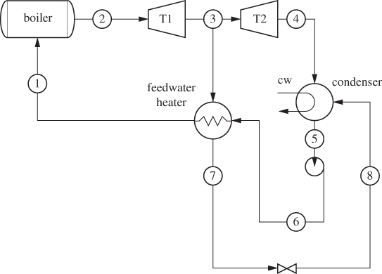
Figure 6-18: Process flow diagram for problem 6.29.
Problem 6.30: Design a vapor compression refrigeration unit using R290 as the refrigerant. The unit must be capable of pumping 1.5 refrigeration tons of heat at −25 °C. The condenser will be operated using water at 25 °C. Determine the flow rate of the refrigerant and the coefficient of performance assuming the compressor to operate with 80% efficiency. Additional information: One standard refrigeration ton is 12,000 BTU/h (3,517 W).
Problem 6.31: The process shown in Figure 6-19 is part of a chiller unit that uses water as the refrigerant. The following data are available: stream 1 is a vapor-liquid mixture at 0.5 bar; stream 5 is saturated vapor at 5 °C; stream 6 is at 500 °C; stream 7 is at 100 °C. Calculate the following on the basis of 1 kg/s of water in stream 1:
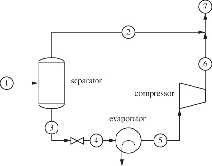
Figure 6-19: Process flow diagram for problem 6.31.
a) Calculate the energy balances.
b) Determine the rate of entropy generation and identify the irreversible units in order of significance.
c) Show the process on a qualitative PH graph.
Problem 6.32: Methyl chloride at 2 bar and 65 °C is to be liquefied under constant pressure to produce saturated liquid.
a) Calculate the ideal work for this process assuming the surroundings to be at 25 °C.
b) The liquefaction will be carried out using a refrigeration cycle with a coefficient of performance ω = 3.5. Calculate the work needed to operate this cycle.
c) What is the lost work for the cycle in part (b)?
The following information for methyl chloride is available: Saturation temperature at 2 bar: −7 °C. ΔHvap at 2 bar: 21.5 kJ/mol. CP of vapor: 38 J/mol K. Assume CH3Cl vapor may be assumed to be ideal. Is this a good assumption?
Problem 6.33: A standard vapor compression cycle uses tetrafluoroethane as the refrigerant. The refrigerant at the exit of the condenser is saturated liquid at 90 °F; at the exit of the evaporator it is saturated vapor at 0 °F. The cycle is powered by a compressor rated at 5 hp. The coefficient of performance of this cycle is 2.5.
a) How much heat is removed in the evaporator?
b) What is the flow rate of the refrigerant?
c) What is the entropy generation?
d) What is the efficiency of the compressor?
NOTE: 1 hp = 2545 Btu/h.
Problem 6.34: You are designing a refrigeration cycle that will absorb 100 W of heat at −10 °F. The cycle will use ammonia as the refrigerant in a standard vapor compression cycle. Its condenser will be cooled by air, assumed to be at 80 °F. Calculate the energy balances, determine the flow rate of the refrigerant, and calculate the entropy generation. Assume a 10 °F temperature between streams in the heat exchangers and a compressor efficiency of 80%.
Problem 6.35: An air-conditioning system, powered by solar energy, is being designed to maintain the temperature inside a house at 20 °C against a temperature of 30 °C of the surroundings. Solar panels will be used to heat water to 200 °C and this energy will be used to power the air conditioner. Considering the house, the surroundings, and the water tank to be heat reservoirs, what is the power that must be supplied to run the air conditioner per kW of heat pumped out of the house?
Problem 6.36: Ammonia is liquefied in a steady-state process by first compressing the gas and then cooling until all the ammonia condenses. The cooling takes place in a heat exchanger using water at 90 °F. The ammonia enters the compressor at 80 psia and 80 °F. The efficiency of the compressor is 80%.
a) What is the minimum pressure that we must have at the exit of the compressor in order to achieve liquefaction?
b) Calculate the amount of work in the compressor.
c) Calculate the amount of heat that must be removed by the cooling water.
Problem 6.37: Figure 6-20 shows a two-stage refrigeration cycle with two evaporating temperatures, flash gas removal, and intercooling. The cycle operates using carbon dioxide as the refrigerant. The condenser (HE1) uses cooling water at 25 °C to produce saturated liquid (stream 2). One third of the mass flow rate at 2 is diverted to stream 3 with the remainder going into stream 5. Both evaporators (HE2 and HE3) produce saturated vapor. The flash gas separator (S1) removes all the vapor at the top (stream 8) and the liquid at the bottom (stream 9). The second stage HE3 removes heat at the rate of 100 W at −40 °C. Both compressors increase the pressure of their respective incoming streams by the same factor and they both operate with an efficiency of 80%. This system must be capable of removing 100 kW of heat in evaporator HE3. Determine the flow rate of the refrigerant, the amount of work in the compressors, and the heat loads in all heat exchangers. Perform a second-law analysis and identify the unit that contributes most to the irreversible operation of this cycle. Finally, sketch a PH graph and show the states of all streams.
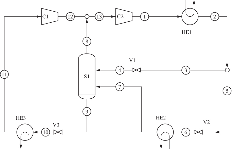
Figure 6-20: Process flow diagram for problem 6.37.
Problem 6.38: The refrigeration cycle in Figure 6-21 shows a vapor compression cycle with recirculation. The vapor-liquid separator after the throttling valve recycles the vapor to the compressor and passes the liquid to the evaporator. This process uses the refrigerant R-134a with the evaporator temperature set at −20 °C, the condenser at 30 °C, and with compressor efficiency of 75%. Determine the energy and entropy balances and compare the efficiency of this process to the simple vapor-compression cycle without recirculation.

Figure 6-21: Process flow diagram for problem 6.38.
Problem 6.39: Natural gas, which you may take to be pure methane, is liquefied in the Claude process shown in Figure 6-22. The process operates between a high pressure of 30 bar and a low pressure of 1 bar. The inlet stream is at 1 bar, 20 °C, compression is to 30 bar, stream 13 is at 3 °C, the precooler uses water to cool the compressed gas to 30 °C, streams 5 and 6 are at 8 °C, and the mass flow rate in stream 2 is 20 times larger than ![]() 1. The efficiency of the compressor and the turbine is 85%. Determine the mass, energy, and entropy balances on the basis of 1 kg of liquified natural gas, and report the actual and ideal work. Discuss the features of this process compared to the Linde process.
1. The efficiency of the compressor and the turbine is 85%. Determine the mass, energy, and entropy balances on the basis of 1 kg of liquified natural gas, and report the actual and ideal work. Discuss the features of this process compared to the Linde process.
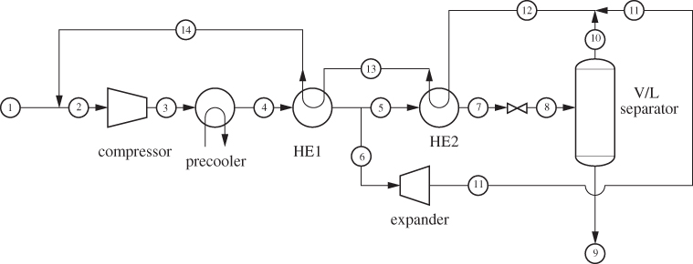
Figure 6-22: Process flow diagram for problem 6.39.
Problem 6.40: Design a Linde process to liquefy oxygen. Pure oxygen is supplied at 1 bar, 25 °C and liquid oxygen is received at 1 bar. The fluid is compressed to 150 bar in a series of compressors whose efficiency is 80%. Precooling is done by water at 20 °C. Compression in done in stages with intercooling, to maximum temperature of 200 °C. Perform the energy balance and a second-law analysis of the process.
Problem 6.41: Oxygen is compressed from 1 bar, 25 °C, to 150 bar. To avoid overheating, compression is done in stages followed by intercooling with water at 30 °C so that the temperature exiting each stage of the compressor does not exceed 200 °C. Using data from the NIST WebBook, determine the number of stages, the work in each stage, and the amount of cooling, if the efficiency of all stages is 80%.
Problem 6.42: A 3 m3 insulated tank contains steam at 1 bar, 150 °C. The tank is connected to a steam line that is maintained at 10 bar, 300 °C until the pressure in the tank is 5 bar. How much steam (kg) was transferred into the tank and what is the final temperature in the tank?
Problem 6.43: A 5 m3 insulated tank contains steam at 10 bar, 200 °C. Three kilograms of steam is removed by venting to the atmosphere (1 bar, 20 °C). What is the pressure and temperature in the tank after venting?