Chapter 4. Entropy and the Second Law
The first law, discussed in the previous chapter, expresses a fundamental principle, energy conservation. All processes observed in nature are bound to satisfy this principle. To put this differently, a process is physically impossible if it violates the first law. The opposite, however, is not true: not every process that satisfies the first law is in fact possible. Consider this familiar situation: if we throw a piece of ice in warm water and leave the system undisturbed, the ice will melt and the water will become colder. This process satisfies the first law, as the amount of energy that is absorbed by the ice is equal to the energy (heat) rejected by the warm water. Now, consider the same process in reverse: a glass of water spontaneously produces the original piece of ice floating on warm water. Such a process does not violate the first law, if all the heat that leaves the ice goes to make the rest of the water warm. Yet, this process is impossible. We can of course, separate the liquid into two parts, freeze one, heat the other, then put them together to produce the original system. However, such a process is not spontaneous; to take place it requires our intervention. By contrast, the melting of ice in the original experiment requires no such intervention whatsoever. There are numerous similar examples of processes that take place spontaneously in one specific direction but never in the opposite one: oxygen and nitrogen placed into contact with each other will mix without further interference from the outside but air does not spontaneously unmix into oxygen and nitrogen; a bouncing ball must eventually come to rest by converting its kinetic energy into internal energy, but a ball at rest will not spontaneously begin to bounce by converting some of its internal energy into kinetic energy; and so on. These situations fall under the same general paradigm: a system brought to state A and left undisturbed reaches state B; but if the same system is brought to state B and is left undisturbed, it will not reach A. Since the process A → B is observed to take place, it obviously satisfies the first law. This means that the process B → A satisfies the first law as well; yet it does not take place. We conclude that there is another principle at work that determines whether a process that satisfies the first law is indeed possible or not. This principle is known as the second law of thermodynamics and in its heart lies entropy, the most fundamental concept in thermodynamics.
What You Will Learn in This Chapter. In this chapter we formulate the mathematical statement of the second law for a closed system and learn how to:
1. Calculate entropy changes of real fluids along special paths.
2. Determine, after the fact, whether a process was conducted reversibly or not.
3. Apply the first and second law to determine if a proposed process is thermodynamically feasible.
4. Apply the notion of a cycle to determine thermodynamic efficiency.
4.1 The Second Law in a Closed System
To fix ideas, consider the following experiment: an insulated cylinder is divided by a movable wall into two compartments, one that contains a hot pressurized gas, and one that contains a colder, low-pressure gas (state A). The separating wall, which is conducting, is held into place with latches. The latches are removed and the system is left undisturbed to reach its final equilibrium state (state B), which, experience teaches, is a state of uniform pressure and temperature across both compartments. This process is spontaneous and adiabatic. Our development is motivated by the tendency of isolated systems like this to reach equilibrium. This tendency defines a preferred direction: towards the equilibrium state, never away from it. We recognize that such directionality cannot be represented by an equality; it requires an inequality so that if it is satisfied in one direction it is violated in the opposite one. At equilibrium, this inequality must reduce to an exact equality, so that the direction of change is neither forward nor backward—without this special condition, a system would never reach equilibrium. Moreover, the quantity in the inequality that fixes this direction must be such that if its change is positive in one direction, it will be negative in the opposite direction, so that the process may proceed in one direction only. It must, therefore, be a state function. Finally, since the state of a nonequilibrium system is nonuniform but consists of various parts in their own local states, the property we are after must be extensive, so that all parts of the system contribute to the determination of the direction to equilibrium. With these ideas in mind we formulate the second law as follows:
Since entropy is a state function, a small change dS is expressed as the difference S2 − S1 between two neighboring states; it follows that for a step in the reverse direction, the entropy change is S1 − S2 = −dS. In other words, if the entropy change is positive in one direction, it is negative in the opposite: the direction of the process at each step is unambiguously revealed by entropy.
Relating Entropy to Measurable Quantities
For entropy to be of any practical value, we must be able to relate it to quantities that can be measured experimentally. Here is how we develop this relationship. Since entropy is a state function, we can express it as a mathematical function of two intensive properties. We choose internal energy U, and volume V, and write S = S(U, V). This unusual choice is perfectly permissible.1 The differential of entropy in terms of these independent variables is
1. This choice of state variables is not arbitrary but guided by the process in Figure 4-1. An isolated system exchanges neither heat nor PV (or other) work with its surroundings. Its internal energy and volume, therefore, remain constant. The conditions of constant internal energy and constant volume, which appear in the partial derivatives in eq. (4.4), represent the external constraints imposed to the process depicted in Figure 4-1.
This is a general equation for the change of entropy following a differential change of state. We will apply it to a mechanically reversible process. We begin by expressing dU from the first law, dU = dQrev + dWrev, and use dWrev = −PdV:
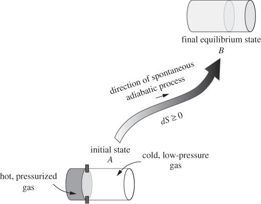
Figure 4-1: Spontaneous adiabatic process: equilibration between two parts initially held at different pressure and temperature.
dU = dQrev − PdV,
We substitute this result in eq. (4.4), which now takes the form
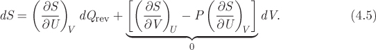
The quantity in square brackets is zero by virtue of eq. (4.2): in the special case of reversible adiabatic process (dQrev = 0) dS must be zero and the only way to satisfy this condition is if the bracketed quantity is identically equal to zero. As the last step we define the absolute temperature as the inverse of the partial derivative that is multiplied to dQrev in the above equation:
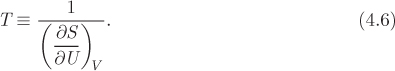
Applying this definition to eq. (4.5) we obtain an important relationship between entropy, heat and temperature:

With this result we have related entropy to measurable quantities (heat, temperature). We now have a simple methodology to calculate entropy changes between two states: connect the states with a mechanically reversible path, and compute the quantity dQrev/T along a differential step. The change of entropy between the two states is the integral of this differential over the entire path:
Since entropy is a state function, any reversible path will yield the same result. Therefore, the choice of the path is not important and this allows us to choose according to convenience. The fact that entropy, a state function, is related to heat, a path function, should be no reason for concern: different paths will yield different amounts of heat (and different increments dQrev along the way) but the integral of dQrev between two points must yield the same value regardless of path.2 Equation (4.7) also reveals the units of entropy: in extensive form it has units of energy divided by temperature (kJ/K); its intensive form is usually reported in kJ/kg K or J/mol K.
2. If still unconvinced, recall that the equation for the reversible work can be written as dV = −dWrev/P, thus relating volume (a state function) to reversible work (a path function).
Note
Entropy and Temperature
In eq. (4.6) we identified the partial derivative (∂S/∂U)v with 1/T. We rewrite this as

and adopt it as the formal definition of absolute temperature. It is not obvious why this partial derivative represents the familiar temperature, but then again, we have not provided, until now, any formal definition of temperature beyond the qualitative (“gives rise to the sensation of hot and cold”). We will establish this equivalency through demonstrations that show the above definition is fully consistent with our intuitive notions of temperature. For instance, in Example 4.15 we show that heat flows from higher to lower temperature (and not the other way around), and in Section (4.9) that temperature at equilibrium is indeed uniform throughout the system.
4.2 Calculation of Entropy
Constant-Pressure Path, No Phase Change
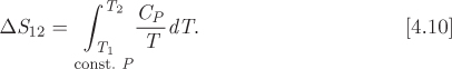
A rather simple problem is the calculation of ΔS between two states at the same pressure. To perform this calculation we devise a reversible constant-pressure path between the two states. If no phase change occurs, the heat along this path is
dQ = dH = CPdT.
With this result, eq. (4.8) becomes
This equation gives the entropy difference between two states at the same pressure but at different temperatures. Since entropy is a state function, it does not matter whether the actual process that brought the system from the initial state to the final was a constant-pressure process, some more complicated path, or even an irreversible process. The integration path used to calculate a state function between two states, and the actual path that took the system from the initial state to the final, are entirely independent.
Equation (4.10) may be expressed in simpler form by making use of the log-T mean heat capacity, introduced in eq. (3.47). Then, the entropy change is
If the heat capacity does not vary much over the temperature interval from T1 to T2, then ![]() . In this case, entropy may be calculated from eq. (4.11) with the log-T mean heat capacity replaced by CP.
. In this case, entropy may be calculated from eq. (4.11) with the log-T mean heat capacity replaced by CP.
Constant-Volume Path, No Phase Change
A similar equation can be written for a path of constant volume with no phase change. In this case the heat is
dQ = dU = CV dT
and the entropy change is

This can also be written in the simpler form,
where ![]() is the log-T mean constant-volume heat capacity.
is the log-T mean constant-volume heat capacity.
dQ = CPdT.
CP/R = a0 + a1T + a2T2,
a0 = 16.8559 a1 = − 0.0183185 a2 = 8.35939 × 10⁻⁵.
Numerical substitution with T1 = 285.15 K, T2 = 328.15 K, gives ![]() J/mol K and the corresponding entropy change is
J/mol K and the corresponding entropy change is
CP = 15.354 − 0.116117T + 0.000451T2 − 7.842 × 10⁻⁷T3 + 5.206 × 10⁻¹⁰T4,
SA ≈ SL(100 °C) = 1.307 kJ/kg K.
Entropy of Solids and Liquids
The entropy of incompressible phases (solids, liquids far from the critical point) is nearly independent of pressure. Entropy in this case depends only on temperature and may be calculated using eq. (4.10), even if pressure is not the same in the two states.
Entropy and Phase Change
The entropy of vaporization is defined as the difference between the entropy of saturated vapor and saturated liquid:
The entropy of vaporization has a simple relationship to the enthalpy of vaporization. We begin with eq. (4.8), which we apply across the tie line from saturated liquid to saturated vapor. Along this path T is constant and Q = ΔHvap. Therefore,
Consider now a point inside the vapor-liquid region (point C in Figure 4-2). It represents a mixed-phase system with a fraction xL of liquid and xV of vapor. The entropy of this state is obtained by adding the contributions of the liquid and vapor fractions:
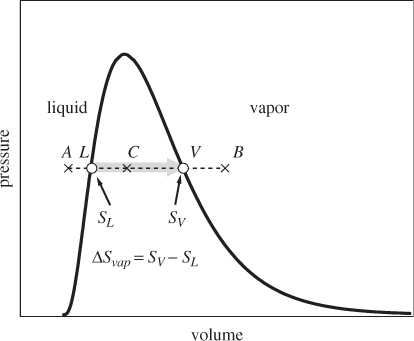
Figure 4-2: Entropy change during vapor-liquid transition.
Using xL + xV = 1 we solve this equation for xL and xV and find,
This is the familiar lever rule. It applies here because entropy is an extensive property.
SL = 1.3070 kJ/kg K, SV = 7.3541 kJ/kg K.
ΔSvap = SV − SL = (7.3541 − 1.3070) kJ/kg K = 6.0471 kJ/kg K.
CP/R = a0 + a1T + a2T2 + a3T3 + a4T4,

ΔHvap = 32883.4 J/mol.
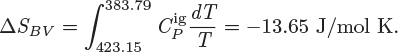
1. Cooling from initial vapor state to saturated vapor (BV). The entropy change for this part is
2. Condensation of saturated vapor to saturated liquid (VL). The entropy for this part is the negative of the entropy of vaporization:
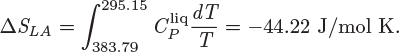
3. Cooling of saturated liquid at constant pressure (LA). The entropy change for this part is
ΔS = −13.65 − 85.68 − 44.22 = −143.55 J/mol K.
ΔS = ΔSBV − xLΔSvap = −13.65 − (0.53 × 85.68) = −59.05 J/mol K.
Entropy Change of Bath
A heat bath is a system so large that its temperature does not change in any appreciable amount when it absorbs or rejects heat. The entropy change is calculated using eq. (4.10). Since temperature is constant, the integral reduces to
where Qbath is defined with respect to the bath, that is, positive if added to the bath, negative otherwise. Usually, the bath is part of the surroundings, used as a heat source or sink for the system of interest. In situations like this, heat is calculated with respect to the system and has the opposite sign. The entropy change of the bath, expressed in terms of the heat of the system, is
where Q = −Qbath is the heat defined with respect of the system. The example below illustrates this calculation.
Tip
Entropy of Bath
In writing eq. (4.19) we assume that the heat has been calculated with reference to the system. Another way to write the same equation is in the form
with the + sign if the bath receives the heat from the system, and the − sign if it transfers it to the system. It follows that when the bath absorbs heat its entropy increases, and when it rejects heat its entropy decreases. Use this result as a check whenever you perform a bath calculation.
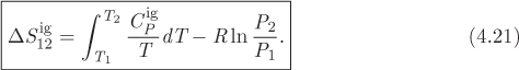
Entropy in the Ideal-Gas State
In the previous sections we demonstrated the calculation of entropy between two states at different temperature but the same pressure. The more general calculation between any two states will be presented in Chapter 5. Here, we show that such general calculation is quite simple in the special case that both states are in the ideal-gas state. Consider two states, 1 and 2, on the PT plane, as in Figure 4-3. We construct a two-step mechanically reversible path, first at constant pressure to final temperature T2 (state 2′), then at constant temperature to final pressure P2. The calculation of entropy will be performed along each step separately using eq. (4.8) and the results will be added at the end.

Figure 4-3: Path for the calculation of entropy changes in the ideal-gas state.
Along branch 12′, pressure is constant, therefore, eq. (4.10) applies:

Along branch 2′2, the process is isothermal, as well as mechanically reversible. Application of the first law gives
dUig = dQrev − PdVig.
The change in internal energy in the ideal-gas state is given by eq. (3.34), and since temperature is constant, dUig = 0. Therefore, the amount of heat is
dQrev = PdVig.
We use the ideal-gas law to write Vig = RT/P; differentiation at constant temperature gives
The heat, therefore, is
The entropy change along this step is now calculated by applying eq. (4.8) with the above result for the heat:
The entropy change between states 1 and 2 is ![]() , or,
, or,
Using the log-T mean heat capacity (see eq. [3.40]), this result can also be expressed as
The log-T mean heat capacity may be replaced by ![]() if the heat capacity does not vary much with temperature in the interval T1 to T2.
if the heat capacity does not vary much with temperature in the interval T1 to T2.
Using Tabulated Values
Finally, as a state function, entropy can be tabulated. The steam tables in the appendix include the specific entropy of water in the saturated region (liquid, vapor) and in the superheated vapor region. If tabulated values are not available, then entropy changes may be calculated from eq. (4.8). The calculation requires the amount of heat that is exchanged along the path and this is generally obtained by application of the first law. This methodology is applied below to a number of special cases.
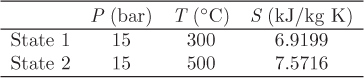
ΔS12 = S2 − S1 = (7.5716 − 6.9199) kJ/kg K = 0.6517 kJ/kg K.
4.3 Energy Balances Using Entropy
Equation (4.7) relates entropy to temperature and heat. If this equation is solved for heat, we obtain,
This equation can be used to calculate the amount of heat, provided that the process is mechanically reversible. The full amount of heat for a process is given by the integral of this differential from initial to final state:
This equation has a simple graphical interpretation on the TS graph: heat in a mechanically reversible process is equal to the area under the path (Figure 4-4). The relationship of heat to temperature and entropy is analogous to the relationship of work to pressure and volume, and further illustrates the fact that heat is a path function. Heat is positive if the path moves in the direction of increasing entropy (from left to right), and negative if the path is in the direction of decreasing entropy. If the path is closed, that is, the process is a cycle that returns the system to its initial state, the net amount of work is equal to the area enclosed inside the path. This is shown easily by noting that the area DCC′D′ in Figure 4-4 is positive, during step AB, but negative during step CD, and thus is canceled. This result applies to any closed path, not just the rectangular paths because any arbitrary closed path can be represented by a series of interconnected thin (differential) rectangular cycles. A rectangular cycle on the TS graph, operating reversibly, is known as a Carnot cycle and is discussed in more detail in Section 4.5.

Figure 4-4: Paths on the TS graph: (a) open path—this process adds heat to the system; (b) closed path (cycle)—in clockwise direction this cycles absorbs a net amount of heat equal to the area inside the cycle and produces an equal amount of work; (c) Carnot cycle; it consists of two isothermal parts, AB, CD, and two isentropic segments, BC, DA.
The TS plane offers yet another way of representing the thermodynamic state of a system. On this plane, isotherms are shown by horizontal lines, while vertical lines represent lines of constant entropy (isentropic lines). Along an isentropic line, dS = 0; according to eq. (4.7), this condition is met if a process is a mechanically reversible adiabatic process. Thus we conclude that a reversible adiabatic process is also isentropic.
Reversible Adiabatic Process in the Ideal-Gas State
The entropy of ideal gas is given in eq. (4.22). For an isentropic process, ΔSig = 0. Applying this condition to eq. (4.22) we obtain a relationship between pressure and temperature along the isentropic path:

The last result is identical to the one obtained in Section 3.8 (see eq. [3.44]). Therefore, the path of the reversible adiabatic process can be derived either through application of the first law, as was done in Section 3.4 of Chapter 3, or by applying the isentropic condition, as was done here.
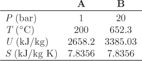
W = ΔUAB = (3385.03 − 2658.2) (kJ/kg) = 726.83 kJ/kg.

with T in kelvin. Equation [A] must be solved numerically for the final temperature. One way to do this by iteration is as follows: as an initial guess, use ![]() and calculate the final temperature from eq. [A]; using this temperature calculate a new value of
and calculate the final temperature from eq. [A]; using this temperature calculate a new value of ![]() and calculate a new temperature from eq. [A]. This procedure is repeated until temperature does not change appreciably any more. These iterations are summarized below:
and calculate a new temperature from eq. [A]. This procedure is repeated until temperature does not change appreciably any more. These iterations are summarized below:


ΔUAB = W + Q.

4.4 Entropy Generation
A system and its surroundings constitute the universe, a closed adiabatic system. For such system the inequality of the second law applies, and thus we have
According to this result, when a system undergoes a process, the net change of entropy in the system and its surroundings is positive, if the process is irreversible, or zero, in the special case of a reversible process. This nonnegative change represents a net generation of entropy,
The second law may then be expressed as
which may be stated as follows:
All processes must result in nonzero entropy generation; a process that results in negative entropy generation is not feasible.
The entropy generation for a process is calculated by combining the entropy changes of all parts of the universe that were affected by the process. Suppose that a system undergoes a differential process during which it exchanges the amount dW and dQ with the surroundings. The entropy generation is
dSgen = dSsys + dSsur ≥ 0.
Treating the surroundings as a bath at temperature T′, its entropy change is
Its precise amount depends on the temperature T′, and increases as the temperature difference between system (at temperature T) and surroundings (T′) increases.3
3. If the heat is removed from the system (dQ < 0), the temperature of the surroundings must be lower than that of the system (T′ ≤ T) and we get
If the heat is added to the system (dQ > 0), the bath temperature must be higher (T′ > T) and the same inequality holds. That is, the surroundings make the smallest possible contribution to entropy generation when the temperature is the same as that of the system.
The best case corresponds to T′ = T, such as, when the bath has the same temperature as the system:
Since dSgen ≥ 0, the above results leads to the following inequality for the entropy change of the system:
To reach these inequalities we assumed that heat transfer between system and surroundings is reversible (i.e., T = T′). If it is not, dS is even larger (according to eq. [4.27]) and the inequality is even stronger. This inequality arises from mechanical irreversibilities within the system. If all processes inside the system are done reversibly, then the inequality reduces to an exact equality and the two expressions in eq. (4.28) revert to eqs. (4.7) and (4.8), as they should.
Note
Entropy of the Universe and Irreversibility
Entropy generation is the net change of entropy in the universe as a result of a process. This total entropy can never decrease; it stays constant, if the process is reversible. Otherwise it must increase. Entropy is a state function and the monotonic increase of entropy means that the universe as a whole cannot return to its previous state, following an irreversible process. This is precisely why we refer to such processes as irreversible. Irreversibility must always be understood with respect to the entire universe. Parts of the universe can be restored to their previous states, but this can only be done at the expense of other parts, whose states must change. When expressed in such stark terms, the relentless march of entropy to ever-higher values with no possibility of return sounds as a harsh principle that imposes a severe limitation to what is possible in nature. Such arguments eventually turn into philosophical inquiries on the relationship between entropy and the irreversible passage of time, and ultimately about human perception of physical reality. It is not our intention to follow that road, fascinating as it may be. When its various implications make the meaning of entropy fuzzy, it is useful to return the starting point and interpret entropy as the physical property that points evolving systems towards their state of equilibrium.
4.5 Carnot Cycle
The first law introduces the notion that matter is a medium for energy storage: energy can be added in the form of either heat or work, and is stored as internal energy. This energy can be later extracted in the form of a combination of heat and work. This is precisely what the steam engine does: water absorbs heat and in the process it becomes pressurized steam; work is extracted through the expansion of the steam. A practical question of engineering relevance is, can all of the heat that enters the system be recovered as work? If not, what is the maximum possible fraction that can be recovered? To address the question of “maximum” work, we must first establish a baseline. This baseline is provided by the notion of thermodynamic cycle. A cycle is any process that returns the system back to the same state where it was found initially. Why use a cyclic process as a baseline? Consider the analogous problem in accounting: Two people receive loans from the bank and invest the money in various projects. To determine who made more money, the loans must be repaid first. This amounts to restoring the system (the bank) to its initial state. Neglecting to do this would lead to meaningless comparisons since the person with the largest debt could claim to be the richest of the two. The notion of the cycle requires us to consider the costs of restoring the system to its original state before we can make pronouncements of efficiency.
A special cycle of fundamental theoretical importance is the Carnot cycle, depicted graphically in the TS graph in Figure 4-5. It is a reversible cycle that consists of two isothermal branches, AB and CD, and two isentropic branches, BC and DA. The isothermal branches are one at high temperature TH, and one at lower temperature TL(TH > TL).

Figure 4-5: (a) Carnot cycle on the TS plane; (b) pictorial representation of the Carnot cycle.
The cycle may be implemented experimentally. We examine each portion of the path separately.
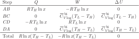
1. Isothermal step AB. This step represents reversible isothermal heating. The amount of heat in this part is given by eq. (4.24). Noting that temperature is constant, this heat is
Since SB > SA, this heat is positive and must be added to the system. This step also involves some amount of PV work (WAB), as volume changes due to heating.
2. Isentropic step BC. This step represents reversible adiabatic expansion. During this step the system produces an amount of work, WBC.
3. Isothermal step CD. This step is the reverse of that in AB and represents reversible isothermal cooling. The amount of heat is
The system also exchanges PV work (WCD) due to volume changes that occur with cooling.
4. Isentropic step DA. This is the reverse of step BC. It represents reversible adiabatic compression during which the system absorbs an amount of work, WDA.
These heat and work exchanges are indicated by the arrows in Figure 4-5 that show the direction of the exchange.
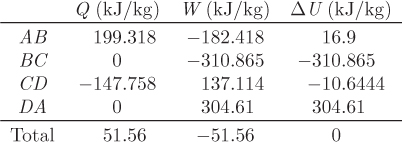
First-Law Analysis of the Carnot Cycle
The overall energy balance along the path ABCDA is
where Q and W are the net amounts of heat and work, respectively. Over a complete cycle along the path ABCDA, the system is returned to its original state; therefore, the change in internal energy is zero:
ΔU = 0.
The net amount of heat is the sum of the amounts exchanged with the two baths:
Q = QH + QL.
The net amount of work is the sum of the work exchanged in each part:
W = WAB + WBC + WCD + WDA.
If the net amount is negative, then there is net production of work; if the net amount is positive, the cycle consumes work, that is, it requires work in order to operate. In the remainder of the calculation it is the net amount of work that we will be interested in, not the individual contributions in each step.
Second-Law Analysis of the Carnot Cycle
The entropy change of the system is zero because its state is restored at the end of one cycle:
ΔSsys = 0.
The entropy of the surroundings is affected in the two baths that exchange heat with the system. The entropy change in each of these baths is given by eq. (4.19):
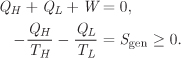
Since the Carnot cycle is reversible, the entropy generation is zero:
We solve this equation for QL, substitute the result into eq. (4.31) and solve the resulting equation for the work. We find
The heat QH is positive (see eq. [4.29]); so is the quantity in the parenthesis, because TH > TL. This makes the net work negative, in other words, work is produced by the cycle. This cycle is a heat engine: It receives heat from a source at high temperature TH and produces a net amount of work.
Thermodynamic Efficiency
In addition to producing a net amount of work, the cycle produces an amount of heat QL, which it rejects to the surroundings at the lower temperature TL. The fraction of the input heat that is converted into work is from eq. (4.33),4
4. Since W is negative, −W is the absolute value of the work produced.
Since TL < TH, the right-hand side is less than 1. We conclude that the cycle cannot convert the entire amount of heat it receives into work. Moreover, the fraction of heat that is converted into work depends only on temperature, but it is independent of the physical properties of the fluid. The Carnot efficiency, η, is defined as
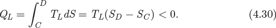
and gives the fraction of the heat that enters the Carnot cycle at the temperature of the hot reservoir that is converted into work. The remaining fraction is rejected as heat at the lower temperature TL. It is not possible to exceed the efficiency of the Carnot cycle: Given two heat reservoirs, one at TH and one at TL, the maximum fraction of the heat that enters the cycle is solely a function of the two temperatures and is given by eq. (4.35). The proof is straightforward. The entropy generation of any cycle that exchanges heat with the two reservoirs is
from which we obtain
Applying the first law on this cycle and solving for QL we obtain
0 = QH + QL + W ⇒ QL = −QH − W.
Combining the two results and solving for the ratio −W/QH we find
On the left-hand side we have the efficiency of the unspecified cycle, while on the right-hand side we have the efficiency of the Carnot cycle. That is,
with the understanding that all cycles are restricted to exchange heat with the same two reservoirs. The equal sign applies if the unspecified cycle operates reversibly. We recognize now that the Carnot efficiency is achieved when a cycle is operated reversibly between two heat reservoirs. Exceeding the Carnot efficiency is not possible because it would amount to negative entropy generation, which is equivalent to a spontaneous process that moves an isolated system away from equilibrium.
Real power plants operate differently from the Carnot cycle but the big picture is the same: An energy source at high temperature is used to supply heat to a process, whose net result is to produce an amount of work. In industrial production of power the heat source is either a fossil fuel such as coal or a nuclear fuel. In either case a chemical or nuclear reaction releases heat at an elevated temperature, which acts as the high-temperature reservoir. Invariably, part of this heat must be rejected to the surroundings but at a lower temperature. As a result, only a fraction of the heat released by the fuel is converted into work. The Carnot efficiency gives the maximum possible fraction of work that can be extracted, given the temperature of the heat source and the heat sink (usually the surroundings). The efficiency of real processes is lower than the theoretical efficiency because of irreversibilities that cannot be avoided in practice.
The technical reasons for the unavoidable rejection of heat at the lower-temperature reservoir will become more clear when we consider actual cycles in Chapter 6. The fundamental reason, however, is evident in Figure 4-5. According to eq. (4.30), the amount of heat QL is equal in absolute value to the area DCC′D′. Clearly, it is impossible to complete the cycle without rejecting this amount of heat at the lower reservoir. The area is zero only if TL is equal to absolute zero, and in this case the Carnot efficiency becomes 1. For any other value of TL, the amount of QL is nonzero and the efficiency of the cycle less than 1. In practice, TL is fixed by the temperature of the ambient surroundings. It is possible of course to produce temperatures lower than ambient using refrigeration, but we will see in Chapter 6 that this requires work and cancels the benefit from the higher efficiency of the cycle.
WDA = CV(TH − TL).

ΔU = Q + W.
Note
Entropy, Reversibility, and Real Processes
In Chapter 1 we introduced the notion of the quasi-static process and explained that such process is also reversible. The second law provides us with an independent and unambiguous way to determine whether a process is reversible or not: If entropy generation is positive, the process is irreversible; if it is zero, the process is reversible. If the entropy generation is negative, the process cannot take place as described. The only information that is required are the initial and final states of the system and of the surroundings. It is not necessary to know the path, nor how the process was conducted (quasi-statically or not). In other words, the second law allows us to characterize a process as reversible or irreversible by examining the state of the universe before and after a process. Since “quasi-static” implies “reversible” and vice versa, when a process results in entropy generation one must be able to identify gradients that give rise to irreversibilities. Similarly, if gradients are identified, one must expect an entropy analysis to show positive generation. Why are such processes irreversible? One answer to this question was given in Chapter 1, where we explained that only a quasi-static process can be reversed and retrace its exact path in either direction. The second law provides us with a different way to view this question. Since entropy is a state function, generation of entropy means that the state of the universe after an irreversible process is different. And since restoring the state of the universe would require negative entropy generation, such process is not feasible. In other words, the initial state of the universe cannot be restored following an irreversible process.
The impossibility of restoring the effects of irreversible processes may appear as a dramatic statement to some, but there is nothing controversial about it. It simply restates in quantitative terms what we know by experience to be true, namely, that spontaneous processes are driven by gradients. More specifically, they are driven by the dissipation of gradients: A hot system and a cold system exchange heat and during the process their temperatures come closer together; a pressurized gas expands against surroundings at a lower pressure and during this process the pressures come closer together; a blob of ink spreads in water and the composition of the solution becomes more uniform.5 At the end of these processes, the universe as a whole has moved closer to equilibrium by erasing some gradients that existed before. It is possible, of course, to reintroduce gradients in a uniform system: through heating and cooling we can create temperature gradients in an equilibrated system; a gas can be divided into parts of which one may be compressed, the other expanded, to produce a pressure difference; ink and water can be separated and then remixed to produce a concentrated blob. All of these processes, however, require the exchange of energy, which may only come at the expense of other gradients. In other words, to restore those parts of the universe that were affected as a result of an irreversible process is possible only by altering the state of other parts.
5. As we will learn in Chapter 10, the spreading of the ink blob is driven by gradients in the chemical potential of the ink and the water. These gradients are being erased by the diffusion process.
A reversible process is a special process that allows us to take advantage of gradients without losing them to dissipation. Suppose that an amount of heat Q must be added to a system at temperature T. This heat must be available at some higher temperature T′. Normally, we would place the two systems into thermal contact until they exchange the required amount of heat. This process is irreversible and results in positive entropy generation, as we found in Example 4.15. Here is one way to achieve this heat transfer reversibly. Operate a Carnot cycle between temperatures T′ and T such that the amount of heat that is rejected at T is equal to Q. This process accomplishes two things: It delivers the required amount of heat to the system, but also produces a certain amount of mechanical work. This work may be used to reverse the process (transfer heat from the system at T to the bath at higher temperature), or to produce other gradients elsewhere in the universe (e.g., compress a gas). From this perspective, an irreversible process represents a lost opportunity to produce work. It is this aspect of irreversibility that is of relevance in thermodynamics because it attaches a “work penalty” to irreversibility. In general, a process that produces work will produce less than the maximum possible amount, if conducted irreversibly. A process that consumes work will consume more than the minimum theoretical amount under irreversible conditions. The best case scenario (maximum amount of work produced, minimum amount of work consumed) corresponds to the minimization of entropy generation, that is, to the reversible condition, Sgen = 0.
4.6 Alternative Statements of the Second Law
The second law is expressed in many equivalent forms and different textbooks adopt different statements. We will discuss some of these in order to provide a connection to statements you may find in the thermodynamics literature and to show how these are consistent with the approach taken here.
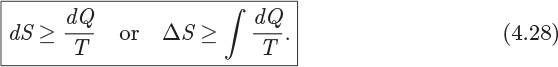
Alternative statement 1: For any change of state, the following inequality holds true:
This becomes an exact equality if the process is reversible.
We recognize this as eq. (4.28), which we derived previously. In many textbooks this is the preferred statement of the second law because the relationship between entropy and heat is immediate and does not require additional derivations. The problem with approach is that this inequality must be accepted without any physical justification. Mathematically, however, this statement is completely equivalent to our definition: for an adiabatic process, eq. (4.28) indeed reduces to eq. (4.3) and from there on, we recover all of the other results obtained in this chapter.
Two statements of historical significance are given below. One is due to Rudolph Clausius, the other due to William Thomson (Lord Kelvin) and Max Planck:
Alternative statement 2 (Clausius): It is not possible to construct a device whose sole effect is to transfer heat from a colder body to a hotter body.
Alternative statement 3 (Kelvin-Planck): It is not possible to construct a device that operates in a cycle and whose sole effect is to produce work by transferring heat from a single body.
These statements express the second law in terms of observations that may be defended through our empirical knowledge of the physical world. The Clausius statement essentially states the impossibility of spontaneous heat flow from lower temperature to higher temperature. The key condition in this statement is that such transfer cannot be “sole effect” of the device. This leaves room for refrigerators, which require work to pump heat from lower temperature to higher temperature. Absent such energy input, heat cannot travel from low to high temperature. The Kelvin-Plank statement states that the efficiency of a power cycle cannot reach 1. It can be shown that starting with either one of these statements we obtain eq. (4.2). The example below outlines the equivalence between the Clausius statement and the fundamental inequality of the second law. If these derivations sound complicated, lengthy, and indirect it is because they follow the historical development of entropy. It is a credit to the intellect of Carnot, Clausius, Kelvin, and Planck that they were able to discover entropy without the benefit of our modern understanding of thermodynamics, based only on observations of irrefutable physical behavior.

1. First, show that no cycle can exceed the efficiency of the Carnot cycle. This is done as follows. Suppose that a cycle between temperatures TH and TL < TH exceeds the efficiency of a Carnot cycle between the same two temperatures. We reverse the Carnot cycle to operate as a refrigerator and use the work produced by the super-efficient cycle to power this refrigerator. By energy balance, this arrangement is shown to transfer heat from the low-temperature bath to the high-temperature bath. Since this arrangement does not receive work from the surroundings (the work transfer from the super-efficient cycle to the Carnot refrigerator is an internal transfer when the two cycles are taken to the system), it violates the Clausius statement. Therefore, no cycle can exceed the efficiency of the Carnot.
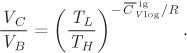
2. Next, show that the efficiency of a Carnot cycle that operates using an ideal gas as the working fluid is
This calculation was done already in Example 4.11 by applying the first law alone, that is, without making any references to entropy, which in the Clausius approach has not been defined yet.
3. Show that the integral
is independent of the integration path, that is, it represents a state function. To do this, we first point out that the equation for the Carnot efficiency can be expressed in the form
Next we consider two interconnected Carnot cycles, as in Figure 4-6. When both cycles operate in the same direction (both clockwise, or both counterclockwise), their common part is canceled and the combined cycle is represented by the outline that encloses the two cycles, a closed path. This cycle exchanges heat with four baths, two at elevated temperatures (TH1 and TH2) and two at lower temperatures (TL1 and TL2). For this combined cycle, the above relationship between amounts of heat and temperature becomes

Figure 4-6: A cycle composed of two interconnected Carnot cycles. Using enough reversible adiabatic paths close to each other, any reversible closed path can be represented by a series of Carnot cycles. Along such closed path, the integral of dQrev/T is zero (see Example 4.14).
This we write in the more compact form as
where Qrev is the amount of heat that is absorbed by the system divided by the temperature of the system (for reversible heat transfer, the temperature of the bath matches the temperature of the system), and the summation is over all heat baths with which the system exchanges heat. If the reversible adiabatic paths are drawn close enough, any arbitrary closed path can be represented by a series of infinitesimally small Carnot cycles, each of which exchanges an amount dQrev of heat with a bath at T. The previous result then is generalized to
which states that the integral of the quantity Qrev/T over a closed path is zero. This result implies that this integral, calculated between two states A and B, is independent of the integration path: if the integral did depend on the path, then going from A to B and returning back to A through different paths would yield a different result each time. But as we showed already, the integral must be zero along any closed path. We conclude that the integral of dQrev/T is independent of the path, therefore, it must be a state function. This defines entropy:
4. The efficiency of an irreversible cycle operating between temperatures TH and TL, is less than that of the Carnot cycle between the same two temperatures. This condition is equivalent to the inequality
which, carried through the previous derivation leads to
This can also be written as
For this result to be true along any closed path, we must have
But the right-hand side is dS; therefore, this result reads
For an adiabatic process, this becomes
Note
Carnot Cycle and the “Work Value” of Heat
From an end-user perspective we can understand that heat and work are not equivalent in the sense that work is more highly valued than heat. Suppose we are given an amount of heat Q at temperature T. How much work can we extract from that amount? If we have access to a reservoir at lower temperature T0 (and the surroundings are always a convenient choice), then we can build a cycle between T and T0 and feed the amount Q into it to produce work. In this sense, the temperature difference is equivalent to a voltage difference in an electric circuit, or elevation difference in a gravitational system (a river flowing to sea level from a mountain spring), and provides an opportunity to produce work. If the power cycle is reversible, the fraction of heat that is converted into work is the Carnot efficiency, 1 − T0/T. The balance will appear as heat that is rejected at T0; this amount can no longer be converted into work unless a reservoir at an even lower temperature becomes available. In this sense, the “work value” of the amount of heat Q is
There are two important observations to make here: first, that the work value is always less that the amount of heat itself; and second, that the work value of heat depends on the temperature at which the heat is available and increases with increasing temperature. Sometimes we express this second point by saying that the quality of heat decreases as its temperature gets closer to that of the surroundings. The practical conclusion is that the usefulness of heat depends on its temperature. For example, if 100 kJ is available at 40 °C, we could use it to melt ice but not to boil water. That is, this heat is not as useful at 40 °C as it would be at, say 200 °C.
4.7 Ideal and Lost Work
We now want to answer the following question: How much work is necessary to change the state of a fixed amount of a substance from some initial state A to a final state B? Work is, of course, a path function, so the answer must depend on the specific path. Let’s say that the change of state requires the consumption of work. Clearly, there is no upper limit to the amount of work that can be consumed because we can always devise arbitrarily long paths to reach the final state. But is there a minimum amount of work that is needed to produce this change? The answer must be yes, because, even if the change of state can be achieved entirely through heating with no direct input work, that heat has a corresponding price in terms of work.
To perform this calculation we adopt a path that takes the system from the initial to the final state using a single reservoir at T0 for all heat exchanges. This reservoir can be used either as sink or as a source of heat. We can do that by setting up a cycle between T0 and the system at T: If the heat transfer is in the direction of the lower temperature, the cycle will operate as an engine and will produce some work; if the transfer is in the direction of the higher temperature, then work will have to be consumed to move the heat against the temperature difference. Starting with the first law we have
ΔU = Q + W,
where W is the net amount of work and includes the work in the cycle operating between the system and the reservoir. By second law, the entropy generation is
where ΔS is the entropy change of the system and −Q/T0 is the entropy change of the surroundings. We solve the second law for Q, substitute into the first law and solve for the work:
Since entropy generation is always positive, the term T0Sgen adds to the work that must be done. The minimum amount of work corresponds to Sgen = 0, or to a reversible process. This amount of work is called ideal:
and depends on the initial and final states and also on the temperature of the reservoir—but not on the path of the process. The term T0Sgen, which represents extra work that must be done due to irreversibilities, is called lost work:
Returning to eq. (4.38) we may express the actual work W in terms of the ideal and lost work in the simple equation,
If the change of state requires work to take place (e.g., W > 0), the ideal work represents the minimum amount that must be consumed. If the change of state produces work (e.g., W < 0), the ideal work represents the maximum amount (in absolute value) that can be produced. In both cases, the lost work represents a penalty due to irreversibilities. If the process consumes work, the lost work is an extra amount that must be offered. If the process produces work, the lost work subtracts from the amount that could be produced.6 In this sense, “lost” work refers to a lost opportunity to produce more work.
6. Recall that the lost work is always positive but work produced in negative. Then, the actual work produced can be written as
The corresponding equation for a process that consumes work is
In this form it is clear that the lost work always represents a penalty.
ΔUAB = Q + W ⇒ Q = ΔUAB − W,
Q = (2582.9 − 3386.1) kJ/kg − (−1200) kJ/kg = 396.8 kJ/kg.

−W ≤ T′ΔS − ΔU.
−W ≤ (473.15 K) × (7.6147 − 8.1557) (kJ/kg K) − (2582.9, − 3386.1) kJ/kg = 547.2 kJ/kg.
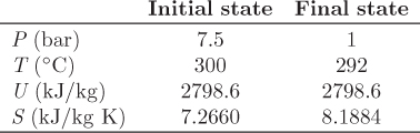
Sgen = ΔSsur + ΔSsys = 0 + (8.1884 − 7.2660) kJ/kg K = 0.9224 kJ/kg K.

4.8 Ambient Surroundings as a Default Bath—Exergy
The ideal work for a process that changes the state of the system depends on the temperature of the surroundings, which play the role of heat source and heat sink for all the heat requirements of the process. In most situations, heat will usually be available at an elevated temperature, for example, at the flame temperature produced when natural gas is burned. One must observe, however, that even natural gas must first be brought from ambient conditions to the conditions of the flame, and this requires some additional effort and the expenditure of energy. More generally we should view the surroundings as a baseline state to which all other states tend if left unattended. If we leave a cup of hot coffee or a glass of iced water on the kitchen table, both will equilibrate with the temperature of the surroundings. And a car tire, given enough time, will leak and equilibrate with the pressure of the ambient air. These processes are driven by the tendency of systems to reach equilibrium. It is possible, of course, to remove a state from ambient conditions, but this now requires energy: to make hot coffee we must burn a fuel, to make iced water we need to power a refrigerator, to blow air in a tire we need a compressor. How much work is needed to remove a unit mass of a substance from ambient conditions T0, P0, to final temperature T and pressure P? The answer is given by the ideal work for the state change (T0, P0) → (T, P):
W = (U − U0) − T0(S − S0).
For an expanding system (P > P0), this is the work that can be extracted from the process. For a system under compression (P < P0), it is the work required for the compression. Part of that work, −P0(V − V0), to be specific, is associated with PV work on the surroundings. In expansion, this is the work to push the surroundings by (V − V0); in compression, this is work done by the surroundings towards the compression. If we subtract this work from the ideal work above we are left with the work that is available to us, the human operators of the process. We call this work exergy, or available work, or simply availability:
The term exergy derives from “ex(ternal)” and ergon (Greek for “work”) and implies the useful amount of work that can be extracted from the process, if the process produces work (by contrast, “energy,” which derives from en (Greek for “in”) and ergon, refers to the total amount of stored energy). The term available work refers to the same idea. Equation (4.42) summarizes in a concise way the “attractive pull” of the surroundings. A system at the state of the surroundings has zero exergy and indeed, it is in no position to produce any work. To produce a deviation from this default state we must consume work. Though not immediately obvious from this equation, the exergy is always positive, which means that work must be supplied to the system in order to remove it from the pull of the surroundings.

Exergy, Entropy Generation, Lost Work
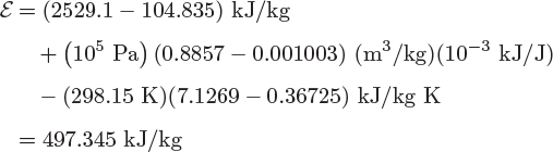
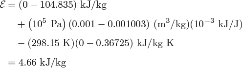
Exergy is the ideal work to bring the system from ambient conditions to the current state (excluding the PV work associated with the surroundings). It is also equal to the maximum amount of useful work that can be produced when the state reverts to ambient. More generally, if the state changes from (T1, P1) to (T2, P2), the corresponding reversible work is the change in exergy between the two states:
Wrev = ε2 − ε1.
If the process is done reversibly, then the above reversible work is also equal to the actual work. In practice, irreversibilities will cost a work penalty equal to T0Sgen that adds to work that must be supplied, and subtracts from the work that can be produced. Exergy, therefore, offers a way to assess the magnitude of irreversibilities, and in that sense it is equivalent to an analysis based on entropy generation. The use of exergy is common in processes whose main focus is to produce mechanical or electrical work. In the study of chemical processes we will use entropy generation as a way to assess irreversibilities and we will report the results in terms of lost work, T0Sgen, because then entropy generation is translated into units of work, which makes it much easier to appreciate its magnitude.
4.9 Equilibrium and Stability
We started this chapter by postulating the existence of entropy based on the undisputable observation that isolated systems have the tendency to reach a state of equilibrium. We return to this idea to show that entropy, via the second law, specifies in precise terms what we mean by equilibrium. To draw this connection, we start with eq. (4.9) to express the bracketed expression in eq. (4.5) in the form,
With this and eq. (4.6), the differential of entropy in eq. (4.4) is written in the simpler form,
Let us now revisit the process in Figure 4-1. The system consists of two compartments, I and II, that can exchange energy via the partition, which is conducting and movable. The energy and volumes of the two parts satisfy the conditions
UI + UII = UI+II = constant,
VI + VII = VI+II = constant,
which follows from the fact that the overall system is insulated and its volume is constant. We may view the equilibration process between the two compartments as an exchange of energy (i.e., by changing the temperature in each compartment) and volume (by moving the partition) under the conditions that the total energy and volume are constant. Suppose that the amount of energy δU and the amount of volume δV are transferred from side II to side I. The entropy change in each compartment and in the total system are obtained from eq. (4.43):
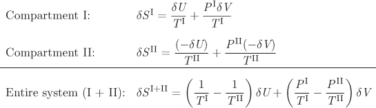
If this transfer of energy and volume causes the entropy of the entire box to increase (i.e., δSI+II > 0), it means that the system is still on its way to equilibrium. At equilibrium, δSI+II = 0. For δSI+II to be zero for small but arbitrary transfers of energy and volume between the two compartments, the multipliers of δU and δV in the above equation must be zero:

from which it also follows that
PI = PII.
We conclude from these equations that when the system reaches equilibrium, temperature and pressure must be uniform throughout the system. That is, entropy, as defined above, leads to the correct equilibrium conditions of thermal and mechanical equilibrium.
Equilibrium Conditions at Constant Temperature and Pressure
In an isolated system (constant energy, constant volume, and constant number of moles), the equilibrium state is the state that maximizes entropy:
(ΔS ≥ 0)U, V, n.
In many practical situations we are dealing, not with isolated systems, but with systems that interact in various ways with their surroundings. An important case is a closed system that interacts with a bath at temperature T under constant pressure P. To study the equilibrium conditions for such a system, we apply the second law to the system and its surroundings:
Using Q = ΔH (recall that the process occurs under constant pressure), this becomes
TΔS − ΔH = TSgen.
We now introduce a new thermodynamic property, the Gibbs free energy, G, which we define as follows:
For an isothermal process, such as the one considered here, the change in the Gibbs free energy is
Combining these results we obtain
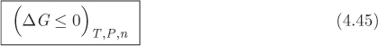
ΔG = −TSgen ≤ 0.
This result states that during the process the Gibbs free energy decreases (ΔG is negative) until equilibrium is reached, at which point G does not change any more (ΔG is zero). In other words, the Gibbs free energy at equilibrium is at a minimum. Mathematically,
This result is the mathematical condition of stable equilibrium. It may not be immediately obvious how it is possible to minimize G while keeping T, P and n constant. After all as a state function, the Gibbs free energy is fixed once T, P and n are specified. Here are some problems where the minimization of the Gibbs free energy is relevant:
• When a pure system can exist in more than one phases, as when the equation of state has multiple roots, the stable phase is identified as the one with the lowest Gibbs free energy. This is discussed in more detail in Chapter 7. In this case, both phases are at the same pressure and temperature, but each has its own value of the Gibbs free energy. The stable phase is the one with the lower Gibbs free energy.
• When a multicomponent system consists of multiple coexisting phases, the compositions in each phase are such that the Gibbs energy is the lowest possible. This is the basis for the calculation of multicomponent phase equilibrium and is discussed in Chapter 10.
• When a mixture is brought to conditions that species can react to produce new species, the equilibrium composition is the one that minimizes the Gibbs free energy.7 This application is discussed in Chapter 14.
7. In this case it is the total mass (or number of atoms), rather than the number of moles that remains constant.
The inequality in eq. (4.45) is an equivalent statement of the second law. In its original formulation, the second law specifies the equilibrium state of an isolated system (i.e., one of constant Utot, Vtot, and ni) as the state that maximizes entropy. If the system is by its temperature, pressure and moles, the equilibrium state corresponds to minimum Gibbs free energy. Other equivalent criteria can be developed depending on the variables that are used to fix the overall system. These statements are summarized below by the inequalities shown below, in which the superscript tot is dropped for simplicity:
where, A is the Helmholtz free energy, defined as
Here is how to read these results: if we fix temperature (via a bath) and the total volume of a closed system, the equilibrium state minimizes the Helmholtz free energy (eq. [4.46]); if we fix entropy and pressure, the equilibrium state corresponds to minimum enthalpy (eq. [4.47]); if we fix entropy and volume, the equilibrium state corresponds to minimum internal energy (eq. [4.48]). Of these, eq. (4.45) is the most important inequality and the one that we will use repeatedly throughout the rest of this book.
Note
Thermodynamic Potentials
According to the above results, the equilibrium state minimizes a thermodynamic function, G, A, H, or U, depending on the variables that are used to specify the overall state of the system. These inequalities introduce a direct analogy with the potential energy of mechanical systems. In mechanical systems, equilibrium may be interpreted in terms of the potential energy function. If Φ(x) is the potential energy as a function of distance x, the force is
Mechanical equilibrium corresponds to a point of zero force, that is, to a point where the slope of the potential with respect to distance is zero. For stable equilibrium the shape of the potential must be convex, that is, a point of minimum in the potential function. Then, any deviation from that point produces a force that points in the direction of decreasing potential, and thus brings the system back to the minimum. The mathematical requirements for the minimum are
The first condition ensures a point of extremum (minimum or maximum), and the second condition ensures that the extremum is a minimum. The Gibbs free energy plays the role of a thermodynamic potential function at fixed temperature and pressure. By analogy to the mechanical system, the mathematical conditions that define a stable equilibrium state at constant pressure and temperature are:
Equation (4.50) expresses the equilibrium condition (zero “force”), and eq. (4.51) the condition for stability (equilibrium point is at a minimum).
4.10 Molecular View of Entropy
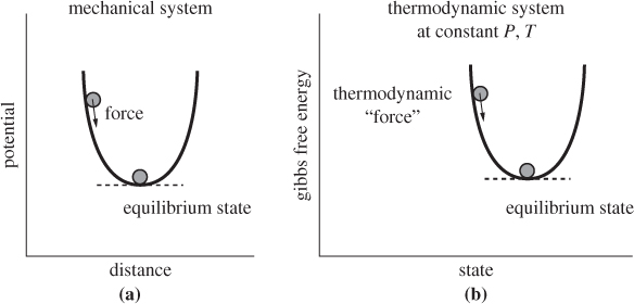
Figure 4-7: Gibbs free energy as a thermodynamic potential.
All of the previous developments of entropy and equilibrium arise from a macroscopic point of view, that is, from the perspective of someone who observes phenomena through their effect on measurable quantities such as pressure, temperature, and the like. It is a fair question to ask, what happens microscopically that gives rise to these macroscopic observations? How do the laws of physics allow a system to approach equilibrium but prevent it from moving away from it? For a molecular perspective we have to turn to statistical thermodynamics. As we mentioned before, a statistical treatment is beyond the scope of this book but this section is offered as a brief glimpse to the physical nature of entropy and the microscopic phenomena responsible for the effects of the second law.
Let us consider again the irreversible expansion experiment: a rigid, insulated tank is divided into two parts that are at different pressures and different temperatures. The partition is removed and the system is allowed to reach an equilibrium state in which pressure and temperature is uniform throughout. It is not very difficult to see the physical mechanism by which pressure becomes equalized. When there is a pressure differential, more molecules cross from the high-pressure part to the low pressure part than in the reverse direction, which cause a net transfer of mass from high pressure to low pressure and a corresponding decrease of the pressure difference. The equilibration of temperatures works in a similar manner: Molecules in hot regions have higher velocities and transfer some of their energy through collisions to slow moving molecules from colder regions of the system. Nature in other words works in ways that tend to erase gradients and ultimately produce equilibrium states characterized by uniform conditions. We view this state as one of higher disorder compared to what we had initially. Right after the partition is removed but before the system has had a chance to establish equilibrium, all the high-pressure molecules are on one side of the tank. This is a state of relatively high order because we know where to look for hot or cold molecules. At equilibrium, molecules are mixed and could be anywhere in the tank. This order/disorder picture may be easier to follow if we assume that the second half of the tank is evacuated before the partition was removed. We view the final state as one of higher disorder because we are less certain where a molecule is, since there is more space where the molecules can be found. The case can be made that spontaneous processes always lead to more disorder. In this view, entropy becomes a measure of disorder.
Statistical mechanics provides us with a precise way to define disorder. In an isolated system of fixed size (volume and mass) and energy, it is in principle possible to enumerate the different instantaneous configurations of molecules inside the system. For example, one configuration can be obtained by placing molecules at random positions in the available space and give each an arbitrary velocity but in such a way that the total energy is equal to the value specified initially. Other configurations can be obtained by shifting around the positions of the molecules and by redistributing the energy among them. Disorder can now be defined as the number of different configurations that are possible under the given conditions, i.e., under the specified size and total energy contained in the system. The larger the number of configurations, the larger the disorder, in the sense that our uncertainty as to which configuration is actually materialized at any point in time increases as the number of possibilities increases. Avoiding for the moment the question of how one could really count the apparently infinite number of such configurations, if that number is Ω, then the entropy of an isolated system is
where kB is Boltzmann’s constant. It can be shown that eq. (4.52) is equivalent to the familiar entropy. Here, rather than a proof, we will provide a demonstration to connect this expression to more familiar results. Viewing entropy as a measure of disorder, there are two contributions that must be accounted for: one comes from changes in the number of ways that the total energy of the system can be divided among all molecules, and the other comes from changes in the number of ways to arrange these molecules in space. We will focus on an isothermal process in the idealgas state. Since energy in the ideal-gas state depends only on temperature, the only contribution we need to consider is that due to the number of arranging molecules in space. To enumerate the number of ways that we can arrange N molecules in a box of volume Vtot we divide the volume of the box into a grid of volume elements of size v0, where v0 is the volume of one molecule, as shown in Figure 4-8. This gives M = Vtot/v0 number of grid elements. From combinatorial algebra we learn that the number of ways to place N identical molecules in M boxes is8
8. You can verify this result by explicitly counting the ways for some small N and M, say, N = 2, M = 4.
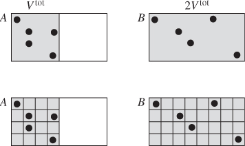
Figure 4-8: Molecular snapshots of a system of molecules at volume Vtot, temperature T (A) and volume 2Vtot, temperature T (B). To enumerate the ways of arranging the molecules in the available volume we subdivide space into a grid of volume elements.
In typical thermodynamic systems N and M are very large numbers, of the order of 1023, give or take a few quadrilion. For such large integers the logarithm of the factorial can be replaced by the following limiting expression,
Taking the logarithm of eq. (4.53), using the above limit we obtain
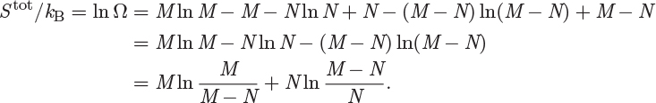
In the ideal-gas state molar density is very low, in other words, there are many more volume grid elements than there are molecules. This means that M ≫ N, and leads to the conditions ln(M/(M − N)) → lnM/M = 0 and ln((M − N)/N) → ln(M/N). Using these results, the entropy takes the form

The number of moles, n, is n = N/NA, where NA is Avogadro’s number. Recalling that R = NAkB, we obtain

where V = Vtot/n is the molar volume and c = v0NA is a constant. Let us now calculate the difference in entropy when the volume changes from V1 to V2. Using the above equation, the entropy change is
If we further write V2/V1 = P1/P2 (recall that both states are at the same temperature), we obtain the familiar result for isothermal entropy change in the ideal-gas state:
The point of this exercise is to show that eq. (4.52), whose basis is entirely molecular, produces the same final result for entropy as the classical macroscopic treatment.
Entropy and Probabilities
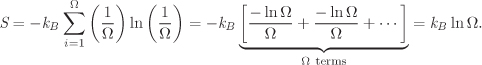
Statistical mechanics provides a more general expression for entropy: if a system can exist in many microscopic states i = 1, 2, ···, Ω, and if the probability to find the system in microstate i is pi, then the entropy of the system is
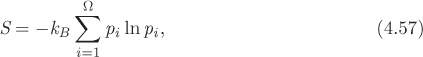
where kB is Boltzmann’s constant and with the summation running through all microscopic states. By “microscopic state” we mean a molecular “snapshot” in time, namely, a specific arrangement of positions and velocities for all molecules. This equation embodies the probabilistic nature of entropy. Equation (4.52) is a special case of eq. (4.57) that is obtained if all microscopic states are equally probable (see Example 4.21). Equation (4.57) gives precise mathematical meaning to the qualitative notion of “disorder,” which should be understood in a probabilistic sense: a system is in a state of higher disorder if the number of possible states where it can be found, weighted by the factor −pi ln pi, increases.9 Statistical mechanics also teaches how to evaluate the probability of microstates in different situations; this, however, is beyond the scope of our treatment.
9. According to eq. (4.57), entropy increases not just by the number of available microstates but by −pi ln pi per microstate. Microstates that are highly probable contribute more than those that have a lower probability.
4.11 Summary
In this chapter we have dealt with two basic problems: One has to do with the various consequences of the second law; the second has to do with how to calculate entropy. We summarize them in reverse order.
Calculation of Entropy
• The basic formula for the calculation of entropy is eq. (4.7),
according to which, entropy is obtained by integrating the quantity dQ/T along a reversible path. The general procedure is to calculate dQ by applying the first law along a step of the process. In the special case that the path is one of constant pressure, the calculation is performed using the heat capacity according to eq. (4.10):
This equation applies provided that there is no phase change. If a phase change does occur, the entropy of vaporization must be included. Since entropy is an extensive property, the usual forms of the lever rule apply.
• Entropy calculations in the ideal-gas state are straightforward. The entropy change between any two states in the ideal gas is
These equations summarize the various ways by which we can calculate entropy. Of course, entropy may also be obtained from thermodynamic tables, if available.
Consequences of the Second Law
The second law imposes an important limitation to all processes in nature: The entropy change in the universe may be zero or positive, but not negative. This requirement points a process always in the direction of equilibrium and has several important implications:
• Unless a process is conducted reversibly, it changes the universe in an irreversible way: the state of the universe cannot be fully restored following such process.
• A process that results in negative entropy generation is not feasible. This is a useful check when we design processes on paper.
• A thermal gradient has the potential to produce work. If an amount of heat is available at temperature TH, a fraction of that heat can be converted into work. The maximum possible fraction that can be converted is given by the Carnot efficiency:
where TL is a lower temperature. The Carnot efficiency refers specifically to a cycle operating between two temperatures, TH and TL.
4.12 Problems
Problem 4.1: Calculate the entropy change of steam between states P1 = 36 bar, T1 = 250 °C, and P2 = 22 bar, T2 = 400 °C by direct application of the definition of entropy. Hint: devise a path of constant pressure followed by a path of constant volume that connects the two states; use tabulated values of U and H to calculate the required heat capacities.
Problem 4.2: A 2 kg piece of copper at 200 °C is taken out of a furnace and is let stand to cool in air with ambient temperature 25 °C. Calculate the entropy generation as a result of this process. Additional data: The CP of copper is 0.38 kJ/kg K.
Problem 4.3: A bucket that contains 1 kg of ice at −5 °C is placed inside a bath that is maintained at 40 °C and is allowed to reach thermal equilibrium. Determine the entropy change of the ice and of the bath. Additional information: CP,liq = 4.18 kJ/kgK, CP,ice = 2.05 kJ/kgK, ΔHfusion = 334 kJ/kg.
Problem 4.4: To convince yourself that the entropy of a bath changes even though its temperature remains unchanged, consider the following case: A tub that contains water at 40 °C receives 100 kJ of heat. Calculate the final temperature of the water and its entropy change if the mass of the water in the tub is:
a) 1 kg.
b) 10 kg.
c) 1000 kg.
d) Compare your results to the calculation ΔS = Qbath/Tbath. What do you conclude? (For water use CP = 4.18 kJ/kg K.)
e) Prove that when the mass of the bath approaches infinity the entropy change of the bath is

Hint: Recall that ln x ≈ x − 1 when x ≈ 1.
Problem 4.5: Ethanol vapor at 0.5 bar and 78 °C is compressed isothermally to 2 bar in a reversible process in a closed system.
a) Draw a qualitative PV graph and show the path of the process. Mark all the relevant pressures and isotherms.
b) Calculate the enthalpy change of the ethanol.
c) Calculate the entropy change of the ethanol.
d) What amount of heat is exchanged between the ethanol and the surroundings during the compression?
Assume that ethanol vapor is an ideal gas with CP = 45 J/K mol. The saturation pressure of ethanol at 78 °C is 1 bar.
Problem 4.6: One mol of methanol vapor is cooled under constant pressure in a closed system by removing 25000 J of heat. Initially, the system is at 2 bar, 200 °C.
a) Determine the final temperature.
b) Calculate the entropy change of methanol.
Additional data: boiling point of methanol at 2 bar: 83 °C; heat capacity of vapor: 60 J/mol K; heat capacity of liquid: 80 J/mol K; heat of vaporization at 2 bar: 36740 J/mol.
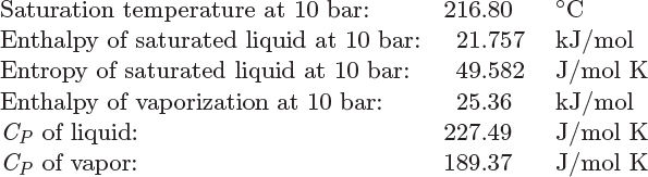
Problem 4.7: Calculate the entropy of toluene in the following states:
a) 10 bar, 300 °C
b) Vapor-liquid mixture at 10 bar with quality 25%.
c) 10 bar, 20 °C.
d) 15 bar, 20 °C.
The following data are available:
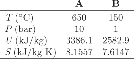
Problem 4.8: Steam is compressed by reversible isothermal process from 15 bar, 250 °C, to a final state that consists of a vapor-liquid mixture with a quality of 32%.
a) Calculate the amount of work.
b) Calculate the amount of heat that is required to maintain isothermal conditions. Is this heat added or removed from the system?
Problem 4.9: Steam in a closed system is compressed by reversible isothermal process in a heat bath at 250 °C, starting from an initial pressure of 15 bar. During the process, the steam transfers 2000 kJ/kg of heat to the bath. Determine the final state and the amount of work involved.
Problem 4.10: Steam in a closed system is compressed by reversible isothermal process in a heat bath at 250 °C, starting from an initial pressure of 15 bar. During the process, the steam receives 400 kJ/kg of work. Determine the final state and the amount of heat exchanged with the bath.
Problem 4.11: Steam at 1 bar, 150 °C, is compressed in a closed system by reversible isothermal process to final pressure of 20 bar. Determine the amount of work and the entropy change of the steam and of the heat bath that is used to maintain the process isothermal.
Problem 4.12: Steam at 1 bar, 150 °C is compressed in a closed system by reversible adiabatic process to final pressure of 20 bar. Determine the final temperature and the amount of work.
Problem 4.13: Nitrogen is compressed adiabatically in a closed system from initial pressure P1 = 1 bar, T1 = 5 °C to P2 = 5 bar. Due to irreversibilities there is an entropy generation equal to 4.5 J/mol K.
a) Calculate the temperature at the end of the compression.
b) Calculate the amount of work. How does it compare to the reversible adiabatic work?
Assume nitrogen to be an ideal gas under the conditions of the problem. Is this a reasonable assumption?
Problem 4.14: Methanol at 2 bar and 65 °C expands isothermally to 0.2 bar through a reversible process.
a) Draw a qualitative PV graph and show the path of the process. Mark all the relevant pressures and isotherms. The process is conducted in a closed system.
b) Calculate the enthalpy change of the methanol.
c) Calculate the entropy change of the methanol.
d) What amount of heat is exchanged between the methanol and the surroundings during the compression?
Assume that the vapor phase is an ideal gas with CP = 45 J/mol K. The boiling point of methanol at 1 bar is 65 °C.
Problem 4.15: Calculate ΔS for steam from 250 °C, 0.05 bar to 250 °C, 6 bar assuming steam to be an ideal gas. Compare to the value in the steam tables.
Problem 4.16: a) Calculate the amount of work necessary for the reversible isothermal expansion of 1 kg of steam from 10 bar to 5 bar at 400 °C.
b) Calculate the amount of heat associated with this process.
Problem 4.17: A rigid insulated tank is divided into two parts, one that contains 1 kg of steam at 10 bar, 200 °C, and one that contains 1 kg of steam at 20 bar, 800 °C. The partition that separates the two compartments is removed and the system is allowed to reach equilibrium. What is the entropy generation?
Problem 4.18: A young engineer notices in her plant that 1-kg blocks of brick are routinely removed from a 800 °C oven and are let stand to cool in air at 25 °C. Conscious about cost-cutting and efficiency, she wonders whether some work could be recovered from this process. Calculate the maximum amount of work that could be obtained. The CP of brick is 0.9 kJ/kg K. Can you come up with devices that could extract this work?
Problem 4.19: A Carnot cycle operating between 600 °C and 25 °C absorbs 1000 kJ of heat from the high-temperature reservoir. The work produced is used to power another Carnot cycle which transfers 1000 kJ of heat from 600 °C to a reservoir at higher temperature TH.
a) Calculate the amount of work exchanged between the two cycles.
b) Calculate the temperature TH.
c) Calculate the amount of heat that is transferred to the reservoir at TH.
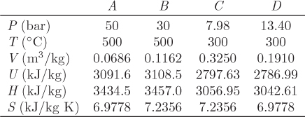
Problem 4.20: A Carnot cycle operates in a closed system using steam: saturated liquid at 20 bar (state A) is heated isothermally until it becomes saturated vapor (state B), expanded by reversible adiabatic process to 10 bar (state C), partially condensed to state D, and finally compressed by reversible adiabatic process to initial state A.
a) Obtain the properties (T, P, V, U, H, and S) at the four states, A, B, C, and D, and summarize the results in a table.
b) Calculate the amount of heat and work involved in each of the four legs of the process.
c) Calculate the net amount of work that is produced.
d) Calculate the ratio of the net work over the amount of heat absorbed at the high temperature of the cycle. How does this value compare to the theoretical efficiency of the Carnot cycle that is calculated based on the two operating temperatures?
Problem 4.21: A Carnot cycle using steam in a closed system operates between 700 °C and 500 °C. During the isothermal step the steam expands from 20 bar to 10 bar. Perform the energy and entropy balances, calculate the efficiency, and compare to the theoretical value.