
Chapter 7. VLE of Pure Fluid
At the vapor-liquid boundary, a single-phase system splits into two phases,1 each with its own properties (molar volume, enthalpy, entropy, etc.). The precise conditions under which phase splitting occurs is an important problem in thermodynamics. Up to this point we have relied on tabulated values and empirical equations, such as the Antoine equation, to establish the relationship between saturation temperature and pressure. In this chapter we develop a connection between the conditions at saturation and the equation of state. The key thermodynamic property that makes this connection possible is the Gibbs energy.
1. A pure substance can form up to three coexisting phases.
The learning objectives for this chapter are to:
1. Calculate the properties of two-phase systems.
2. Use the equation of state to construct the complete phase diagram of a pure fluid.
7.1 Two-Phase Systems
A system at saturation consists of a mixture of two phases. The extensive properties of the mixture are calculated by the lever rule. For the generic property F,
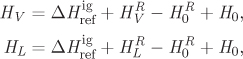
where FL and FV are the properties (specific or molar) of the saturated phases and xL, xV, are the fractions (mass or mole) in each phase (xL + xV = 1). The properties of the saturated phases are calculated by the methods discussed in Chapter 5. The enthalpy of the saturated phases may be calculated from eq. (5.62),
where ![]() and
and ![]() are the residual properties of the saturated phases. These may be calculated from an equation of state, using the liquid root of the compressibility equation for the saturated liquid, and the vapor root for the saturated vapor. The difference between HV and HL is equal to the enthalpy of vaporization. Noting that all other terms on the right-hand side except for
are the residual properties of the saturated phases. These may be calculated from an equation of state, using the liquid root of the compressibility equation for the saturated liquid, and the vapor root for the saturated vapor. The difference between HV and HL is equal to the enthalpy of vaporization. Noting that all other terms on the right-hand side except for ![]() and
and ![]() are common to both equations, the enthalpy of vaporization is simply equal to the difference of the residual terms:
are common to both equations, the enthalpy of vaporization is simply equal to the difference of the residual terms:
The same arguments apply to the entropy of vaporization, for which we find
These results are of practical importance because they allow us to calculate the enthalpy and entropy of vaporization from the equation of state.
Tc = 282.35 K, Pc = 50.418 bar, ω = 0.0866.
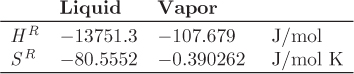
ΔHvap = (−107.679) − (−13751.3) = 13643.6 J/mol,
ΔSvap = (−0.390262) − (−80.5552) = 80.1649 J/mol K.
ΔHvap = 481370 kJ/kg = 13504.4 J/mol.


HV = (2906.5) + (−1802.27) − (−107.679) = 1211.91 J/mol.
HL = (2906.5) + (−10318.7) − (−107.679) = − 7304.48 J/mol.
H = (0.32)(1211.91) + (1 − 0.32)(−7304.48) = − 4579.24 J/mol.
7.2 Vapor-Liquid Equilibrium
Away from the saturation point a fluid exists as a single phase, either liquid or vapor. The saturation point is a special state where the fluid can form both phases, which coexist in equilibrium with each other, both at the same temperature and pressure. We want to determine the precise conditions that define the saturation point. For this we turn to the Gibbs free energy and in particular to eq. (4.45), which states that the equilibrium state of a system at constant T, P, and n is such that the Gibbs free energy is at a minimum. We imagine the following experiment: a fixed number of moles of a fluid is placed in a closed system at such pressure and temperature as to form two phases. The pressure and temperature are then maintained constant (for example, using a movable piston and a heat bath). Suppose that we take a small number of δn moles and transfer them from the liquid to the vapor. The new state is also an equilibrium two-phase system and since the Gibbs free energy is at a minimum, this transfer should cause no change in the total Gibbs free energy of the system. However, the Gibbs free energy of the individual phases changes because G is an extensive property and depends on the number of moles. Specifically, the Gibbs free energy of the liquid changes by −GLδn and that of the vapor by +GVδn. For the total Gibbs free energy to remain constant regardless of the number of moles that are transferred, we must have
This important result states that, while the various molar properties (V, H, S, etc.) are different in the vapor and the liquid, the molar Gibbs free energy is the same in both phases.
Note
Chemical Potential
Equation (7.4) is one of the most important results in equilibrium and places the molar Gibbs energy alongside with pressure and temperature. We may now express the conditions of equilibrium in a single component by stating that pressure, temperature, and molar Gibbs free energy must be uniform throughout the entire system, regardless of the number of phases present.2 For this reason, the molar Gibbs free energy of pure component is also known as chemical potential (symbol μ) because it is the thermodynamic potential of the chemical species at constant T, and P: if the chemical potential in one phase is higher than in another phase, the species will migrate into the phase with the lowest chemical potential; if the chemical potential is the same in two or more phases, then the species can exist with equal probability in any of these phases.
2. Although in the derivation we assumed a vapor-liquid system, the same arguments apply to equilibrium in general, regardless of the number of phases that are present. This is because eq. (4.45) is a general statement of equilibrium and is not restricted with respect to the number or type of phases.
For a pure species, “chemical potential” and “molar Gibbs free energy” are synonymous. For mixtures, as we will find out in Chapter 8, there is a distinction as each component in the mixture has its own chemical potential. With reference to pure species we will continue to use the name “Gibbs free energy” and the symbol G. With reference to a species in a mixture we will use the term chemical potential and the symbol μi.
Clausius-Clapeyron Equation
One consequence of practical significance is that eq. (7.4) provides a relationship between saturation pressure and temperature. To extract this relationship, we return to eq. (5.17), which gives the differential of the Gibbs free energy. We write this equation for the saturated vapor and liquid:
dGV = −SV dT + VV dPsat,
dGL = −SL dT + VL dPsat.
Because the difference between GV and GL is zero, we must have dGV − dGL = 0. Taking the difference between the two equations we have
0 = –ΔSvapdT + (VV − VL)dPsat
and using ΔSvap = ΔHvap/T the result becomes
This is an exact relationship between temperature and pressure at saturation. A practical result is obtained if we make the approximation that the liquid molar volume is negligible compared to the vapor volume (i.e., VV − VL ≈ VV), and that the vapor volume can be calculated by the ideal-gas law (i.e., VV ≈ RT/Psat). Both approximations are acceptable at pressure well below the critical, and both become poor close to the critical point. Using these approximations, the relationship between temperature and saturation pressure becomes
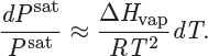
The final approximation is to treat the enthalpy of vaporization as constant. Integrating from (T′, Psat′) to (T, Psat), we obtain the Clausius-Clapeyron equation:
The enthalpy of vaporization is not constant, of course, it decreases with temperature and vanishes at the critical point. Therefore, the above result should be treated as an approximation over short temperature intervals. Despite its approximate nature, the Clausius-Clapeyron equation is useful in that it allows us to calculate the saturation pressure at a temperature, if its value is known at another. According to this equation, the logarithm of the saturation pressure is a linear function of inverse temperature with slope −ΔHvap/R. Saturation pressure is often plotted in semi-log axes against 1/T. In this form the resulting graph is approximately linear.
Antoine Equation
The Clausius-Clapeyron equation can be written as
where A and B are constants. This form suggests that the saturation pressure could be empirically fitted to such linear form. This linearity is, however, subject to the same assumptions used in the derivation, and its validity is limited. To obtain a better empirical fit, a third constant is introduced to write
This is the form of the Antoine equation. It is an empirical equation used to fit experimental data. Its mathematical form, however, is not arbitrary but represents an empirical modification of the Clausius-Clapeyron equation, which turns out to be fairly accurate over an extended range, compared to the equation it is based on. Even so, the Antoine equation cannot accurately fit the entire subcritical region of a fluid.
7.3 Fugacity
The starting point of phase equilibrium is eq. 7.4, which establishes the equality of the molar Gibbs energy of the phases that are present. In this Section we will obtain alternative forms of that equation that are suitable for calculations. First, we express the Gibbs free energy in terms of its residual
G = Gig + GR.
This equation can be written for the liquid and for the vapor. The ideal-gas term is the same in both phases because it depends only on temperature and pressure, which are the same in both phases. We conclude then that the residual Gibbs free energies of the two phases are also equal:
This equation is equivalent to eq. (7.4) but has the advantage that it involves residual properties, whose calculation does not require a reference state. To further streamline the calculation of phase equilibrium we introduce a new property, fugacity, using the following definition:
where ϕ is the fugacity coefficient and is given by
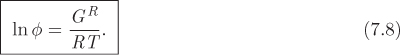
Since the residual Gibbs energy is the same in both phases, the fugacity at saturation satisfies the conditions:
The equality of fugacities is an alternative statement of the necessary and sufficient condition for phase equilibrium and the basis for all such calculations, whether we are dealing with pure substances or with mixtures. By contrast, the equality of the fugacity coefficients is a special result and applies to pure substances only.
Fugacity in the Ideal-Gas State
The limiting values of these properties in the ideal-gas limit follow easily by noting that GR = 0 in this limit:
The fugacity in the ideal-gas limit is equal to pressure, and the fugacity coefficient is equal to unity.
Relationship to the Gibbs Free Energy
The fugacity, an auxiliary property, is related to the Gibbs free energy, the fundamental thermodynamic property at equilibrium. To establish this relationship, first we write the Gibbs energy in the form,
We now take the difference between the Gibbs free energy of two states on the same isotherm:
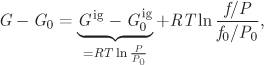
where G, Gig and f refer to state at T, P, while G0, ![]() and f0 refer to state T, P0. Using RTlnP/P0 for the isothermal change of the ideal-gas Gibbs energy between pressures P and P0, the final result is
and f0 refer to state T, P0. Using RTlnP/P0 for the isothermal change of the ideal-gas Gibbs energy between pressures P and P0, the final result is

This establishes the relationship between Gibbs free energy and fugacity, and shows that if we know one of these properties, the other one can be easily obtained. Taking the differential of the above equation at constant temperature, and using eq. (5.17) for dG, the differential of fugacity is
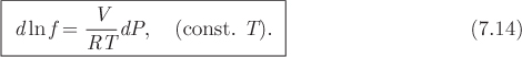
We will use this equation to obtain the variation of fugacity along an isotherm.
Note
Why Fugacity
Fugacity is equivalent to the Gibbs free energy with respect to defining the conditions of phase equilibrium. It offers two practical conveniences over the Gibbs free energy: (a) it does not require a reference state and (b) it has a well-defined (and simple) value in the ideal-gas state. By contrast, the Gibbs free energy requires a reference state, and its value in the ideal-gas state (P → 0) approaches −∞. The name fugacity comes from the Latin fugere (“to flee”) and refers to the tendency of species to “escape” to the more stable phase. It is best to think of fugacity as a defined quantity associated with the Gibbs free energy.
7.4 Calculation of Fugacity
Fugacity is a central property in phase equilibrium. Below we discuss several alternative methodologies that may be used to obtain the fugacity of pure component.
Compressed Liquids—Poynting Equation
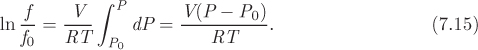
In the compressed liquid region the molar volume is essentially independent of pressure. Equation (7.14) can then be integrated easily to obtain a relationship between the fugacity of a liquid at two different pressures on the same isotherm. With V and T constant, the result is
The term in the right-hand side is known as the Poynting factor. This equation is valid to incompressible phases in general (liquids away from the critical point, and solids in general). A practical result is obtained if we choose the initial state to be the saturated liquid at the given temperature:
where Psat is the saturation pressure, VL, is the molar volume of the saturated liquid, and fL is its fugacity. Using fL = ϕsatPsat, the final result is

This equation allows us to obtain the fugacity in the compressed liquid region from tabulated values at saturation.
f = ϕsatPsat × (1.075) = 0.034 bar.
Using Tabulated Properties
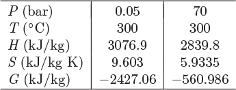
The fugacity is related to the Gibbs energy, which in turn is related to the enthalpy and entropy. It is possible, therefore, to calculate it from tabulated values of H and S. The calculation is demonstrated with the following example.
G = H − TS.
Using the Compressibility Factor
Equation (7.14) gives the fugacity in differential form in terms of volume. It is useful to express this equation in terms of the compressibility factor. Subtracting the term d ln P = dP/P from both sides of that equation we obtain
which we rewrite as
By integration from the ideal-gas state (Z = 1, ϕ = 1) along an isotherm we obtain
According to this result, the fugacity coefficient can be obtained from an integral that involves the compressibility factor. The compressibility factor may be calculated from an equation of state, from tables, or it may be obtained experimentally.
A useful result is obtained if we restrict our attention to the part of the isotherm that is described by the truncated virial equation:
Since the second virial coefficient depends only on temperature and integration along an isotherm, the result is
Using BP/RT = Z − 1, this may be written in a simpler form as
This very simple approximation gives the correct answer in the ideal-gas state and is valid as an extrapolation to pressures sufficiently low that the compressibility factor may be approximated as a linear function of pressure.
f = (0.803)(70 bar) = 56.2 bar.
Fugacity from Generalized Graphs
The residual Gibbs energy can be calculated from the residual enthalpy and entropy. Accordingly, all the methods developed for the residual enthalpy and entropy may be used to calculate GR, and from eq. (7.8) the fugacity coefficient. A quick estimate can be obtained from generalized correlations. Instead of calculating HR and SR individually from Pitzer/Lee/Kesler graphs, separate graphs have been prepared that give the fugacity coefficient by the Pitzer expression,
where (ln ϕ)(0) and (ln ϕ)(1) are universal functions of reduced temperature and pressure. Figure 7-1 shows the term (ln ϕ)(0) calculated by the Lee-Kesler method, as a function of reduced pressure and temperature. This term represents the fugacity coefficient of a simple fluid (ω = 0) and qualitatively resembles the fugacity graph of any pure fluid. All isotherms radiate outward from the ideal-gas state (Pr = 0, ϕ = 1). Isotherms in this region are approximately linear in pressure, as expected on the basis of eq. (7.18). Subcritical isotherms intersect the saturation line and change direction as they pass from one phase into the other. Because ϕL = ϕV at saturation, there is no jump in the value of the fugacity coefficient, however, the slope of the isotherm changes abruptly at this point. The saturation line terminates at the critical point (Pr = Tr = 1). Supercritical isotherms do not intersect with the saturation line. Figure 7-2 shows graphs of (ln ϕ)(0) and (ln ϕ)(1) over an extended range of pressures. Notice that the correction term, (ln ϕ)(1), has a jump across the phase boundary. Since this term is only a correction to a fugacity coefficient, not a fugacity coefficient in itself, the shape of this graph does not convey any physical meaning.
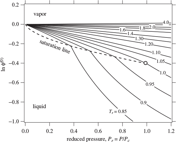
Figure 7-1: Generalized graph for (ln ϕ)(0). The dashed line is the saturation line between vapor and liquid.
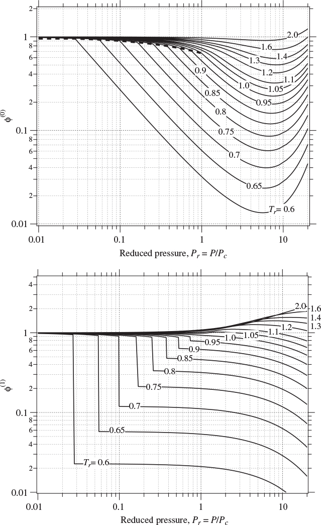
Figure 7-2: Generalized graph for (ln ϕ)(0) and (ln ϕ)(1) (extended range of pressures).
Fugacity from Cubic Equations of State
Writing the residual Gibbs energy as GR = HR − TSR, the fugacity coefficient is expressed as
Therefore, the calculation of the fugacity coefficient by a cubic equation of state does not require much in terms of additional computations, since the required expressions for the residual enthalpy and entropy have been obtained already. In particular, the result for the Soave-Redlich-Kwong and the Peng-Robinson equation are
• Soave-Redlich-Kwong

• Peng-Robinson
In both cases the dimensionless parameters A′ and B′ are given by:
This calculation requires the compressibility factor at the pressure and temperature of interest. If the polynomial equation for Z has three real roots, the proper root must be selected based on the phase of the system.
−0.00216488 + 0.0924639Z − Z2 + Z3 = 0,
Z1 = 0.0401352, Z2 = 0.0599377, Z3 = 0.899927.
ϕ = 0.908246,
f = (0.908246)(15 bar) = 13.62 bar.
7.5 Saturation Pressure from Equations of State
We encountered the following equalities between properties of saturated phases of pure component:
These are equivalent statements of phase equilibrium in a single-component system and any one of them can be used to study equilibrium. Mathematically, the equilibrium criterion is an equation that establishes the relationship between pressure and temperature at saturation:
ϕV (T, Psat) = ϕL(T, Psat).
If temperature is fixed, the saturation pressure may be obtained by solving this equation. This allows us to calculate the saturation pressure via the equation of state of the fluid. Subcritical isotherms from cubic and other analytic equations of state exhibit a metastable/unstable loop (Figure 7-3). The liquid part of the isotherm is represented by the steep branch, labeled AB on this figure, and the vapor part by the gentler branch CD. Points B and C mark the minimum and the maximum of the isotherm. The unstable part of the isotherm between points B and C has been removed. The problem now becomes to locate points L and V, which mark the saturated phases. Numerically, we seek a pressure such that the fugacity coefficients at L and V are the same. This may be done by trial and error. We guess a pressure and solve for the compressibility factor. In this region, there are always three real roots. We use the smallest root to calculate the fugacity coefficient of the liquid and the largest root to calculate the fugacity coefficient of the vapor. If the two fugacity coefficients are not equal, we pick another pressure and repeat until ϕL and ϕV agree to within an acceptable tolerance.

Figure 7-3: Determination of saturation pressure of ethylene using the SRK equation of state.
The fugacity coefficients calculated by this procedure are shown in Figure 7-4. Branches AB and CD correspond to the same ones on the PV isotherm. The liquid fugacity coefficient at high pressures (point A) starts from small values, and increases with decreasing pressure. The fugacity coefficient of the vapor starts at 1 at low pressures and decreases approximately linearly with increasing pressure. At some point the two branches intersect. This defines the saturation point. Figure 7-4 represents a graphical determination of the saturation pressure.
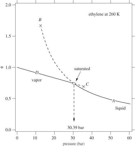
Figure 7-4: Fugacity coefficient of ethylene based on the SRK. Branches AB and CD correspond to the same ones in Figure 7-3.
Note
Stability
As discussed in Chapter 2 (see Section 2.7) the system is mechanically stable over the entire liquid and vapor branches, AB and CD. This means that over the range of pressures bracketed by the pressure of points B and C the system may exist as either vapor or liquid. In regions where a system may exist in more than one phase that satisfies the criteria for stability, the system adopts the most stable phase, rendering the other phases metastable. When two phases are equally stable we obtain the saturation point, namely, a state where two (or more) phases exist in equilibrium with each other. We may identify the stable and metastable phases by comparing their fugacity. Suppose we follow the ϕ isotherm starting from point D. Initially, the compressibility equation has a single root and the only possible phase is the vapor. Beginning with some pressure, the compressibility equation has three real roots, indicating that a liquid phase is possible. However, the fugacity coefficient of this liquid is higher than that of the vapor: the liquid phase is metastable, meaning less stable than the vapor at the same pressure and temperature. A metastable phase may materialize briefly, but thermal fluctuations will eventually cause the system to revert to the more stable phase. At saturation, both phases have the same fugacity coefficient. Past this point, the situation is reversed: the liquid phase is more stable than the vapor because its fugacity coefficient is lower. In all cases the most stable phase is the one with the lower fugacity coefficient. This also means that the more stable phase has lower Gibbs energy, lower residual Gibbs energy and lower fugacity, compared to the metastable phase.3
3. To reach this conclusion we write G = Gig + GR. Since both phases are the same pressure and temperature, the term Gig is common in both phases. Then, the phase with the lower fugacity coefficient has the lower residual Gibbs free energy and also the lower molar Gibbs free energy.
7.6 Phase Diagrams from Equations of State
At this point we have reached one of the main goals we set out to achieve: obtain the properties of a pure fluid at any temperature and pressure. The two pieces of information that make this calculation possible are the equation of state and the ideal-gas heat capacity as a function of temperature. The equation of state allows the calculation of all residual properties and the determination of the phase boundary, namely of the saturation pressure and the properties of the saturated phases. Thus we have the tools to compute the entire phase diagram of the pure fluid. This calculation is demonstrated with the example below.
Z1 = 0.1104, Z2 = 0.2244, Z3 = 0.6651.
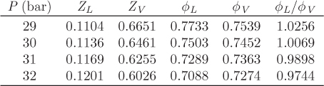
Psat = 30.39 bar.
1. Fix temperature.
2. Calculate the saturation pressure.
3. Fix pressure.
4. Determine the phase of the system at the given pressure: if P < Psat, the phase is vapor; if P > Psat the phase is compressed liquid; if P = Psat, the system is saturated.
5. Solve for the compressibility factor. If three real roots, pick according to the phase.
6. Calculate the residual properties as usual.
7. Calculate the ideal-gas parts of enthalpy and entropy.
8. Combine the ideal gas and residual parts to obtain the absolute properties.
9. Change the pressure and return to step 4 to repeat the calculation.
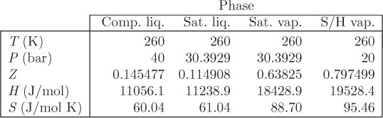
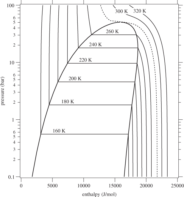
Figure 7-5: Pressure enthalpy graph of ethylene calculated from the Soave-Redlich-Kwong equation (see Example 7.10).
7.7 Summary
In this chapter we developed the theoretical tools for the study of saturated phases, namely, phases that coexist in equilibrium with each other. The fundamental property is the Gibbs free energy, which has the same value in both phases. This fundamental equality is the basis of all the results obtained in this chapter. Fugacity and the fugacity coefficient are auxiliary variables introduced for convenience. They are both related to the Gibbs free energy but are more convenient to work with because they do not require a reference state. In addition, they reduce to very simple expressions in the ideal-gas state.
An important conclusion in this chapter is that all properties of a pure fluid at saturation can be calculated from the equation of state. The equation of state, therefore, along with the ideal-gas heat capacity, provide a complete description of the thermodynamics of a pure fluid. Between the tools developed in the last two chapters we can calculate properties as a function of pressure and temperature at any point of the phase diagram. This benefit comes with one caveat: an accurate equation of state must be available for the fluid of interest. The equations of state discussed here are relatively simple and require a small number of specific properties of the components, namely, critical pressure, critical temperature, and acentric factor. It is quite impressive that such equations provide fairly accurate estimates of various properties. However, the use of these equations should be restricted to normal fluids. Even then, before a serious calculation is undertaken, the equation of state must be rigorously tested against known properties of the fluid. Only then may it be trusted to provide accurate results.
7.8 Problems
Problem 7.1: A pure fluid is described by the Antoine equation
with P in bar and T in kelvin. How much heat is required to evaporate 1 mol of that liquid at 25 °C?
Problem 7.2: Use the steam tables to obtain the fugacity coefficient and ideal Gibbs free energy of steam at 200 bar, 500 °C.
Problem 7.3: a) Calculate the chemical potential of solid acetylene at its triple point. The reference state is the saturated liquid at the triple point.
b) Calculate the change in the chemical potential of the vapor when the pressure is reduced from 1.3 atm to 0.1 atm at the constant temperature of −84 °C.
c) State and justify your assumptions.
Additional data at the triple point: Ttriple = −84 °C, Ptriple = 1.3 atm, Vsolid = 34 cm3/mol, Vliq = 42.7 cm3/mol, Vvap = 12020 cm3/mol.
Problem 7.4: a) Estimate the fugacity of CO2 ice (dry ice) at its triple point (216.55 K, 5.17 bar).
b) Calculate the fugacity of CO2 ice at 216.55 K, 70 bar.
Additional information: density of dry ice: 97.5189 lb/ft3.
Problem 7.5: Use the Lee-Kesler tables to calculate the chemical potential of benzene at the following states:
a) critical point.
b) saturated liquid at 200 °C.
c) 200 °C, 45 bar.
Additional data: The reference state is the ideal gas at 562.1 K, 48.9 bar. The saturation pressure at 200 °C is 14.3 bar.
Problem 7.6: a) A 45-L tank contains 13.5 mol of an unknown gas at 200 °C, 10 bar. Estimate as best as you can the fugacity of the gas.
b) Half of the gas is removed from the tank while maintaining the temperature at 200 °C. Determine the fugacity of the gas that remains in the tank.
Problem 7.7: Use the Pitzer correlation and the Lee-Kesler ϕ tables to calculate the fugacity of ethane at the following states:
a) 1 bar, 40 °C.
b) 50 bar, −70 °C.
Problem 7.8: A fluid that is gas under ambient conditions is stored in a 2 m3 tank. The amount of the gas in the tank is 150 mol. Estimate the fugacity of the gas. State your assumptions clearly.
Problem 7.9: Over a limited range of pressures, an unspecified gas obeys this equation of state,
where a is constant.
a) Derive an expression for the fugacity coefficient.
b) At 30 °C, 1 bar, the compressibility factor of this gas is 0.88. Estimate its fugacity.
c) Calculate the residual Gibbs energy of the gas at 30 °C 1 bar.
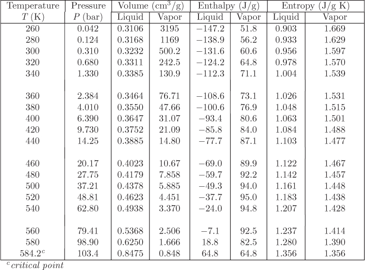
Problem 7.10: The attached table from Perry’s Handbook gives some properties of argon. Using data from this table estimate the following:
a) The fugacity at 300 K, 1 atm (state A).
b) The fugacity of the saturated liquid at 90 K (state B).
c) The ideal-gas Gibbs energy, Gig, of the saturated liquid at 90 K.
d) The fugacity at 50 atm, 90 K (state C).
e) Draw a qualitative PV graph and show the states A, B, and C of the previous parts.
At atmospheric pressure and 300 K, the properties of argon are ρ = 0.0406 mol/L, H = 13919 J/mol, S = 154.82 J/mol K. (see Perry and Chilton, Chemical Engineers’ Handbook 5th ed. (New York: McGraw-Hill, 1973), p. 3-159.)
Problem 7.11: Use the tabulated properties of Br in the table below to do the following:
a) Fugacity at 1 bar, 300 K.
b) Fugacity coefficient of saturated liquid bromine at 1 bar.
c) Fugacity and fugacity coefficient at 150 bar, 300 K.
Note: You may not use generalized correlations for this problem. Use only data given here and make any assumptions you deem appropriate or necessary.
Data for Br2 from Perry’s Handbook, 5th ed., p. 3-159, p. 2-222, Table 2-38
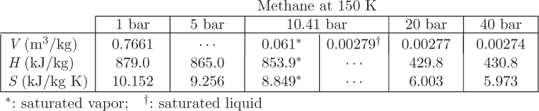
Problem 7.12: Your company faxed you the following table with data for methane at 150 K. A few entries are missing (denoted by “…”) because the fax machine is running out of ink.
a) Is it acceptable to assume ideal-gas state at 1 bar, 150 K? Justify your answer.
b) Calculate the fugacity of saturated liquid at 150 K.
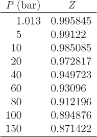
c) Calculate the residual Gibbs energy at 150 K, 60 bar.
d) Calculate the ideal-gas Gibbs energy at 150 K, 60 bar.
Problem 7.13: The table below gives the compressibility factor of ethane at 500 K.
Use this information to obtain the fugacity of ethane at 100 bar, 500 K.
Problem 7.14: The table below shows data for the proprietary molecule X. Use these data to calculate the fugacity of this compound at the following conditions:
a) Saturated vapor at 160 °F.
b) At 200 psi, 160 °F.

Additional data. The critical pressure of this compound is above 500 psi.
Problem 7.15: Some properties of saturated isobutane at 5 bar are given below:
Tsat(5 bar) = 310.5 K, VL = 0.00201585 m3/kg, VL = 0.0783803 m3/kg
Use this information to calculate the following:
a) The fugacity and fugacity coefficient at 0.1 bar, 310.5 K.
b) The fugacity and fugacity coefficient of saturated liquid at 5 bar.
c) The fugacity and fugacity coefficient at 310.5 K, 40 bar.
d) List and justify all of your assumptions.
Problem 7.16: a) Use the SRK equation of state to calculate the saturation pressure of ethane at −58.5 °C.
b) Use the SRK equation to construct the PV graph of ethane. Show isotherms at T = −58.5 °C and T = Tc.
Problem 7.17: Your R&D department works on a proprietary fluid X for which only limited data are disclosed. Among the available information is that the SRK equation at T = 383.3 K, P = 8 bar gives three real roots for Z. These roots and the corresponding residual properties calculated at each value of the three values of Z are listed below:
Based on this information alone, how big of a tank would be needed to store 120 mol of this fluid at T = 383.3 K, P = 8 bar?
Problem 7.18: Use the SRK equation to obtain the saturation pressure of propane at 350 K. Perform the calculation as follows:
a) Determine the highest pressure at which the vapor phase is stable (P1).
b) Determine the lowest pressure at which the liquid is stable (P2).
c) Plot the fugacity coefficient of the vapor starting from a pressure close to the ideal-gas state up to the highest pressure where the vapor is stable. On the same graph make a plot of the fugacity coefficient of the liquid starting from the lowest pressure where the liquid is stable up to some pressure into the compressed-liquid region.
d) Identify the saturation pressure as the pressure where the liquid and vapor fugacity lines cross. How does this result compare with the literature value for the saturation pressure of propane at 350 K?
Problem 7.19: Write a numerical procedure to systematically calculate the saturation pressure of a fluid using the SRK equation of state at a given temperature T. This can be done as follows: First, determine the highest pressure at which the vapor is stable (P′) and the lowest pressure at which the liquid is stable (P″) at temperature T. The saturation pressure is located between these two values. Start with a pressure P between P′ and P″. Obtain the three roots of the compressibility equation at P, T, and use the smallest root to calculate the fugacity of the liquid phase, and the largest root to calculate the fugacity of the vapor phase. If the fugacity of the liquid is lower than the fugacity of the vapor, choose a lower pressure (why?); otherwise choose a higher pressure. Repeat the calculation with the new pressure and continue until the fugacity of the vapor is nearly the same as that of the liquid. Note: At low temperatures P″ may be negative. In this case the saturation pressure is bracketed between P = P′ and P = 0.
a) Use your program to calculate VL, VV, ΔHvap, and ΔSvap of propane at 350 K.
b) Use your program to make a plot of the vapor-liquid boundary on the PV graph.
Problem 7.20: Use the program you wrote in Problem 7.19 to construct a PH graph for propane using as reference state the saturated liquid at 350 K. You may do this as follows: First, obtain the residual enthalpy of the saturated liquid at 350 K. Next, calculate Psat, and the residual enthalpy and entropy of the saturated liquid and saturated vapor at various temperatures between Tc and 250 K. Using these residuals and the specified reference state, calculate the absolute enthalpy of the saturated phases. Plot Psat versus HL and on the same graph plot Psat versus HV. This will give the vapor-liquid boundary. To add isotherms, first tabulate H at various pressures. Start at a pressure close to the ideal-gas state and calculate the enthalpy. If the compressibility equation has three real roots, use the largest one, since the calculation is done for the vapor. Increase the pressure in small steps and repeat the calculation until you reach Psat. Past P = Psat, use the smallest root, since the calculation is now done for the liquid. The isotherm is obtained by plotting the results of this calculation as P versus H.
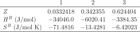
Problem 7.21: The SRK equation gives the following results for toluene at T = 383.3 K, P = 8 bar:

In this table, the first row gives the three roots of the cubic equation for Z, the second row gives the corresponding values of HR, and the third row gives the corresponding values of SR.
a) Report the enthalpy, entropy, and Gibbs energy of toluene at T = 383.3 K, P = 8 bar using as reference state the ideal-gas state at 383.3 K, 40 bar.
b) Calculate the fugacity and the fugacity coefficient at T = 383.3 K, P = 8 bar.
c) Calculate the fugacity at 383.3 K, 40 bar.
Additional data for toluene: Mw = 92.141 g/mol, ω = 0.262, Tc = 591.8 K, Pc = 41.06 bar; boiling point at 1 atm: 383.8 K.