
3. Design to Scale Out Horizontally
Within our practice, we often tell clients that “Scaling up is failing up.” What does that mean? In our minds, it’s pretty clear: We believe that within hyper growth environments it is critical that companies plan to scale in a horizontal fashion through the segmentation of workloads. The practice or implementation of that segmentation often looks like one of the approaches we described in Chapter 2, “Distribute Your Work.” When hyper growth companies do not scale out, their only option is to buy bigger and faster systems. When they hit the limitation of the fastest and biggest system provided by the most costly provider of the system in question they are in big trouble. Ultimately, this is what hurt eBay in 1999, and we still see it more than a decade later in our business and with our clients today. The constraints and problems with scaling up aren’t only a physical issue. Often they are caused by a logical contention that bigger and faster hardware simply can’t solve. This chapter discusses the thoughts behind why you should design your systems to scale horizontally, or out, rather than up.
Rule 10: Design Your Solution to Scale Out—Not Just Up
What do you do when faced with a rapid growth of customers and transactions on your systems and you haven’t built them to scale to multiple servers? Ideally you’d investigate your options and decide you could either buy a larger server or spend engineering time to enable the software to run on multiple servers. Having the ability to run your application or database on multiple servers is scaling out. Continuing to run your systems on larger hardware is scaling up. In your analysis, you might come to the decision through an ROI calculation that it is cheaper to buy the next larger server rather than spend the engineering resources required to change the application. While we would applaud the analytical approach to this decision, for very high-growth companies and products it’s probably flawed. The reason is that it likely doesn’t take into account the long-term costs. Moving from a machine with two 64-bit dual-core processors to one with four processors will likely cost proportionally exactly what you get in improved computational resources (~2x). The fallacy comes in as we continue to purchase larger servers with more processors. This curve of cost to computational processing is a power law in which the cost begins to increase disproportionally to the increase in processing power provided by larger servers (see Rule 11). Assuming that your company continues to succeed and grow, you will continue to travel up the curve in costs for bigger systems. While you may budget for technology refreshes over time, you will be forced to purchase systems at an incredibly high price point relative to the cheaper systems you could purchase if you had built to scale horizontally. Overall, your total capital expenditures increase significantly. Of course the costs to solve the problem with engineering resources will also likely increase due to the increased size of the code base and complexity of the system, but this cost should be linear. Thus your analysis in the beginning should have resulted in a decision to spend the time up front changing the code to scale out.
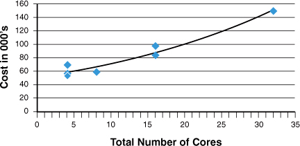
Using an online pricing and configuration utility from one of the large server vendors, the graph in Figure 3.1 shows the cost of seven servers each configured as closely as possible to one another (RAM, disk, and so on) except for the increasing number of processors and cores per processor. Admittedly the computational resource from two dual-core processors is not exactly equivalent to a single quad-core, but for this cost comparison it is close enough. Notice the exponential trend line that fits the data points.
In our experience with more than a hundred clients, this type of analysis almost always results in the decision to modify the code or database to scale out instead of up. That’s why it’s an AKF Partners’ belief that scaling up is failing up. Eventually you will get to a point that either the cost becomes uneconomical or there is no bigger hardware made. For example, we had a client who did have some ability to split their customers onto different systems but continued to scale up with their database hardware. They eventually topped out with six of the largest servers made by their preferred hardware vendor. Each of these systems cost more than $3 million, totaling nearly $20 million in hardware cost. Struggling to continue to scale as their customer demand increased, they undertook a project to horizontally scale their databases. They were able to replace each of those large servers with four much smaller servers costing $350,000 each. In the end they not only succeeded in continuing to scale for their customers but realized a savings of almost $10 million. The company continued to use the old systems until they ultimately failed with age and could be replaced with newer, smaller systems at lower cost.
Most applications are either built from the start to allow them to be run on multiple servers or they can be easily modified to accommodate this. For most SaaS applications this is as simple as replicating the code onto multiple application servers and putting them behind a load balancer. The application servers need not know about each other, but each request gets handled by whichever server gets sent the request from the load balancer. If the application has to keep track of state (see Chapter 10, “Avoid or Distribute State,” for why you will want to eliminate this), a possible solution is to allow session cookies from the load balancer to maintain affinity between a customer’s browser and a particular application server. Once the customer has made the initial request, whichever server was tasked with responding to that request will continue to handle that customer until the session has ended.
For a database to scale out often requires more planning and engineering work, but as we explained in the beginning this is almost always effort well spent. In Chapter 2, we covered three ways in which you can scale an application or database. These are identified on the AKF Scale Cube as X, Y, or Z axis corresponding to replicating (cloning), splitting different things (services), and splitting similar things (customers).
“But wait!” you cry. “Intel’s co-founder Gordon Moore predicted in 1965 that the number of transistors that can be placed on an integrated circuit will double every two years.” That’s true. Moore’s Law has amazingly held true for nearly 50 years now. The problem with this is that this “law” cannot hold true forever, as Gordon Moore admitted in a 2005 interview.1 Additionally, if you are a true hyper growth company you are growing faster than just doubling customers or transactions every two years. You might be doubling every quarter. Relying on Moore’s Law to scale your system, whether it’s your application or database, is likely to lead to failure.
Rule 11—Use Commodity Systems (Goldfish Not Thoroughbreds)
Hyper growth can be a lonely place. There’s so much to learn and so little time to do that learning. But rest assured, if you follow our advice, you’ll have lots of friends—lots of friends that draw power, create heat, push air, and do useful money making tasks—computers. And in our world, the world of hyper growth, we believe that a lot of little low-cost “goldfish” are better than a few big high-cost “thoroughbreds.”
One of my favorite lines from an undergraduate calculus book is “It should be intuitively obvious to the casual observer that <insert some totally nonobvious statement here>”. This particular statement left a mark on me, primarily because what was being discussed was neither intuitive nor obvious to me at the time. It might not seem obvious that having more of something, like many more “smaller” computers, is a better solution than having fewer, larger systems. In fact, more computers probably means more power, more space, and more cooling. The reason more and smaller is often better than less and bigger is twofold and described later in this chapter.
Your equipment provider is incented to sell you into his or her highest margin products. Make no mistake about it, they are talking to you to make money, and they make the most money when they sell you the equipment that has the highest or fattest margin for them. That equipment happens to be the systems that have the largest number of processors. Why is this so? Many companies rely on faster, bigger hardware to do their necessary workloads and are simply unwilling to invest in scaling their own infrastructure. As such, the equipment manufacturers can hold these companies hostage with higher prices and achieve higher margins. But there is an interesting conundrum within this approach as these faster, bigger machines aren’t really capable of doing more work compared to an equivalent number of processors in smaller systems. On a per-CPU basis, there is an inefficiency that simply hasn’t been solved for in these large machines. As you add CPUs, each CPU does slightly less work than it would in a single CPU system (regardless of cores). There are many reasons for this, including the inefficiency of scheduling algorithms for multiple processors, conflicts with memory bus access speeds, structural hazards, data hazards, and so on.
Think about what we just said carefully. You are paying more on a CPU basis, but actually doing less per CPU. You are getting nailed twice!
When confronted with the previous information, your providers will likely go through the relatively common first phase of denial. The wise ones will quickly move on and indicate that your total cost of ownership will go down as the larger units draw less aggregate power than the smaller units. In fact, they might say, you can work with one of their partners to partition (or virtualize) the systems to get the benefit of small systems and lower power drain. This brings us to our second point: We must do some math.
It might, in fact, be the case that the larger system will draw less power and save you money. As power costs increase and system costs decrease, there is no doubt that there is a “right size” system for you that maximizes power, system cost, and computing power. But your vendors aren’t the best source of information for this. You should do the math on your own. It is highly unlikely that you should purchase the largest system available as that math nearly never works. To figure out what to do with the vendors’ arguments, let’s break them down into their component parts.
The math is easy. Look at power cost and unit power consumption as compared to an independent third-party benchmark on system utilization. We can find the right system for us that still fits the commodity range (in other words hasn’t been marked up by the vendor as a high-end system) and maximizes the intersection of computing power with minimal power and space requirements. Total cost of ownership, in nearly all cases and when considering all costs, typically goes down.
On the topic of virtualization, remember that no software comes for free. There are many reasons to virtualize (or in the old language domain or partition) systems. But one never virtualizes a system into four separate domains and ends up with more system processing power and throughput than if you had just purchased four systems equivalent to the size of each domain. Remember that the virtualization software has to use CPU cycles to run and that it’s getting those cycles from somewhere. Again, there are many reasons to virtualize, but greater system capacity in a larger domained system as compared to smaller equivalently sized systems is a fallacy and is not one of them.
What are the other reasons we might want to use commodity systems as compared to more costly systems? We are planning to scale aggressively and there are economies to our rate of scaling. We can more easily negotiate for commodity systems. While we might have more of them, it is easier to discard them and work on them at our leisure than the more expensive systems that will demand time. While this may seem counterintuitive, we have been successful in managing more systems with less staff in the commodity (goldfish) world than in the costly system (thoroughbred) world. We pay less for maintenance on these systems, can afford more redundancy, and they fail less often due to fewer parts (CPUs, for example) on a per-unit basis.
And, ultimately, we come to why we call these things “goldfish.” At scale, these systems are very inexpensive. If they “die,” you are probably incented to simply throw them away rather than investing a lot of time to fix them. “Thoroughbreds” on the other hand represent a fairly large investment that will take time to maintain and fix. Ultimately, we prefer to have many little friends rather than a few big friends.
Rule 12—Scale Out Your Data Centers
The data center has become one of the biggest pain points in scaling for rapidly growing companies. This is because data centers take a long time to plan and build out and because they are often one of the last things that we think about during periods of rapid growth. And sometimes that “last thing” that we think about is the thing that endangers our company most. This rule is a brief treatment of the “how” and “why” to split up data centers for rapid growth.
First, let’s review a few basics. For the purposes of fault isolation (which helps create high availability) and transaction growth, we are going to want to segment our data using both the Y and Z axes of scale presented in Rules 8 and 9, respectively. For the purposes of high availability and transaction growth, we are going to want to replicate (or clone) data and services along the X axis as described in Rule 7. Finally, we are going to assume that you’ve attempted to apply Rule 40 and that you either have a stateless system or that you can design around your stateful needs to allow for multiple data centers. It is this segmentation, replication, and cloning of data and services as well as statelessness that are the building blocks for us to spread our data centers across multiple sites and geographies.
If we have sliced our data properly along the Z axis (see Rule 9), we can now potentially locate data closer to the users requesting that data. If we can slice data while maintaining multitenancy by individual users, we can choose data center locations that are near our end users. If the “atomic” or “granular” element is a company, then we might also locate next to the companies we serve (or at least the largest employee bases of those companies if it is a large company).
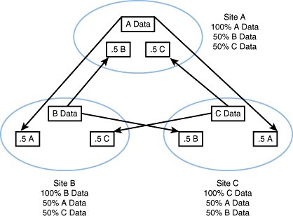
Let’s start with three data centers. Each data center is the “home” for roughly 33% of our data. We will call these data sets A, B, and C. Each data set in each data center has its data replicated in halves, 50% going to each peer data center. Assuming a Z axis split (see Rule 9) and X axis (see Rule 7) replication of data, 50% of data center A’s customers would exist in data center B, and 50% would exist in data center C. In the event of any data center failure, 50% of the data and associated transactions of the data center that failed will move to its peer data centers. If data center A fails, 50% of its data and transactions will go to data center B and 50% to data center C. This approach is depicted in Figure 3.2. The result is that you have 200% of the data necessary to run the site in aggregate, but each site only contains 66% of the necessary data as each site contains the copy for which it is a master (33% of the data necessary to run the site) and 50% of the copies of each of the other sites (16.5% of the data necessary to run the site for a total of an additional 33%).
Figure 3.2. Split of data center replication
To see why this configuration is better than the alternative, let’s look at some math. Implicit in our assumption is that you agree that you need at least two data centers to stay in business in the event of a geographically isolated disaster. If we have two data centers labeled “A” and “B” you might decide to operate 100% of your traffic out of data center A and leave data center B for a warm standby. In a hot/cold (or active/passive) configuration you would need 100% of your computing and network assets in both data centers to include 100% of your Web and application servers, 100% of your database servers, and 100% of your network equipment. Power needs would be similar and Internet connectivity would be similar. You probably keep slightly more than 100% of the capacity necessary to serve your peak demand in each location to handle surges in demand. So let’s say that you keep 110% of your needs in both locations. Anytime you buy additional servers for one place, you have to buy them for the next. You may also decide to connect the data centers with your own dedicated circuits for the purposes of secure replication of data. Running live out of both sites would help you in the event of a major catastrophe as only 50% of your transactions would initially fail until you transfer that traffic to the alternate site, but it won’t help you from a budget or financial perspective. A high-level diagram of the data centers may look as depicted in Figure 3.3.
Figure 3.3. Two data center configuration, “hot and cold” site

But with three live sites, our costs go down. This is because for all nondatabase systems we only really need 150% of our capacity in each location to run 100% of our traffic in the event of a site failure. For databases, we still need 200% of the storage, but that cost stays with us no matter what approach we use. Power and facilities consumption should also be at roughly 150% of the need for a single site, though obviously we will need slightly more people, and there’s probably slightly more overhead than 150% to handle three sites versus one. The only area that increases disproportionately are the network interconnects as we need two additional connections (versus 1) for three sites versus two. Our new data center configuration is shown in Figure 3.4, and the associated comparative operating costs are listed in Table 3.1.
Figure 3.4. Three data center configuration, three hot sites


One great benefit out of such a configuration is the ability to leverage our idle capacity for the creation of testing zones (such as load and performance tests) and the ability to leverage these idle assets during spikes in demand. These spikes can come at nearly anytime. Perhaps we get some exceptional and unplanned press, or maybe we just get some incredible viral boost from an exceptionally well-connected individual or company. The capacity we have on hand for a disaster starts getting traffic, and we quickly order additional capacity. Voila!
As we’ve hinted, running three or more sites comes with certain drawbacks. While the team gains confidence that each site will work as all of them are live, there is some additional operational complexity in running three sites. We believe that, while some additional complexity exists, it is not significantly greater than attempting to run a hot and cold site. Keeping two sites in sync is tough, especially when the team likely doesn’t get many opportunities to prove that one of the two sites would actually work if needed. Constantly running three sites is a bit tougher, but not significantly so.
Network transit costs also increase at a fairly rapid pace even as other costs ultimately decline. For a fully connected graph of sites, each new site (N+1) requires N additional connections where N is the previous number of sites. Companies that handle this cost well typically negotiate for volume discounts and play third-party transit providers off of each other for reduced cost.
Finally, we expect to see an increase in employee and employee related costs with a multiple live site model. If our sites are large, we may decide to collocate employees near the sites rather than relying on remote-hands work. Even without employees on site, we will likely need to travel to the sites from time to time to validate setups, work with third-party providers, and so on. The “Multiple Live Site Considerations” sidebar summarizes the benefits, drawbacks, and architectural considerations of a multiple live site implementation.
Rule 13—Design to Leverage the Cloud
Cloud computing is part of the infrastructure as a service offering provided by many vendors such as Amazon.com, Inc., Google, Inc., Hewlett-Packard Company, and Microsoft Corporation. Vendor-provided clouds have four primary characteristics: pay by usage, scale on demand, multiple tenants, and virtualization. Third-party clouds are generally comprised of many physical servers that run a hypervisor software allowing them to emulate smaller servers that are called virtual. For example, an eight processor machine with 32GB of RAM might be divided into four machines each allowed to utilize two processors and 8GB of RAM.
Customers are allowed to spin up or start using one of these virtual servers and are typically charged by how long they use it. Pricing is different for each of the vendors providing these services, but typically the break-even point for utilizing a virtual server versus purchasing a physical server is around 12 months. This means that if you are utilizing the server 24 hours a day for 12 months you will exceed the cost of purchasing the physical server. Where the cost savings arise is that these virtual servers can be started and stopped on demand. Thus, if you only need this server for 6 hours per day for batch processing, your break-even point is extended for upward of 48 months.
While cost is certainly an important factor in your decision to use a cloud, another distinct advantage of the cloud is that provisioning of the hardware typically takes minutes as compared to days or weeks with physical hardware. The approval process required in your company for additional hardware, the steps of ordering, receiving, racking, and loading a server, can easily take weeks. In a cloud environment, additional servers can be brought into service in minutes.
The two ideal ways that we’ve seen companies make use of third-party cloud environments is when demand is either temporary or inconsistent. Temporary demand can come in the form of nightly batch jobs that need intensive computational resources for a couple of hours or from QA cycles that occur for a couple days each month when testing the next release. Inconsistent demand can come in the form of promotions or seasonality such as “Cyber Monday.”
One of our clients makes great use of a third-party cloud environment each night when they process the day’s worth of data into their data warehouse. They spin up hundreds of virtual instances, process the data, and then shut them down ensuring they only pay for the amount of computational resources that they need. Another of our clients uses virtual instances for their QA engineers. They build a machine image of the software version to be tested and then as QA engineers need a new environment or refreshed environment, they allocate a new virtual instance. By utilizing virtual instances for their QA environment, the dozens of testing servers don’t remain unused the majority of the time. Yet another of our clients utilizes a cloud environment for ad serving when their demand exceeds a certain point. By synchronizing a data store every few minutes, the ads served from the cloud are nearly as up to date as those served from the collocation facility. This particular application can handle a slight delay in the synchronization of data because serving an ad when requested, even if not the absolutely best one, is still much better than not serving the ad because of scaling issues.
Think about your system and what parts are most ideally suited for a cloud environment. Often there are components, such as batch processing, testing environments, or surge capacity, that make sense to put in a cloud. Cloud environments allow for scaling on demand with very short notice.
Summary
While scaling up is an appropriate choice for slow to moderate growth companies, those companies whose growth consistently exceeds Moore’s Law will find themselves hitting the computational capacity limits of high-end, very expensive systems with little notice. Nearly all the high-profile services failures about which we’ve all read have been a result of products simply outgrowing their “britches.” We believe it is always wise to plan to scale out early such that when the demand comes, you can easily split up systems. Follow our rules of scaling out both your systems and your data centers, leveraging the cloud for unexpected demand and relying on inexpensive commodity hardware and you will be ready for hyper growth when it comes!
Endnotes
1 Manek Dubash, “Moore’s Law is dead, says Gordon Moore,” TechWorld, April 13, 2005, www.techworld.com/opsys/news/index.cfm?NewsID=3477.