
Aeroacoustic testing and instrumentation
Abstract
Most experimental testing in aeroacoustics is carried out using wind tunnels. Unless information is required at full scale about a large vehicle or application, running a wind tunnel is usually far less expensive than conducting a field test. It also provides a more controlled environment that can be particularly useful when insight into the fundamental physics is desired. Wind tunnel testing is the focus of this chapter. Some of the different wind tunnel configurations used for low Mach number experimental work are described, as are the acoustic corrections that must be applied to most wind tunnel measurements. This chapter concludes with an overview of some pressure and velocity measurement techniques often used in aeroacoustic testing.
Keywords
Wind tunnels; Acoustic and aerodynamic corrections; Sound and flow measurement
Aeroacoustic predictions must depend to some degree on assumptions or simplifications concerning the physics of sound sources and details of their modeling. Experimental testing provides the most direct way to observe sources, infer their physics, and provide quantitative results against which prediction methods can be validated.
Most experimental testing in aeroacoustics is carried out using wind tunnels. Unless information is required at full scale about a large vehicle or application, running a wind tunnel is usually far less expensive than conducting a field test. It also provides a more controlled environment that can be particularly useful when insight into the fundamental physics is desired. Wind tunnel testing is the focus of this chapter. Some of the different wind tunnel configurations used for low Mach number experimental work are described, as are the acoustic corrections that must be applied to most wind tunnel measurements. This chapter concludes with an overview of some pressure and velocity measurement techniques often used in aeroacoustic testing.
10.1 Aeroacoustic wind tunnels
The ideal aeroacoustic wind tunnel is one that can accurately reproduce the aerodynamics of the device or flow configuration of interest while providing capability for the measurement of the far-field sound that it generates with the minimum of background noise. Accuracy in aerodynamics at low Mach number implies a low-turbulence and closely uniform free stream, model Reynolds numbers that realistically represent the application of interest (which are usually high), and small predictable interference corrections. Aerodynamic interference refers to the differences between the desired flow and the modeled flow which result from the finite extent of the wind tunnel stream. Small corrections allow larger models to be used and thus lead to higher achievable Reynolds numbers.
The standard wind tunnel configuration for aerodynamic studies is the closed test section. Parallel, or nearly parallel, rigid test section walls guide the flow over the model. This type of test section has been in use since at least the time of the Wright brothers and is extremely well understood. Interference corrections are well known and comparatively small and allow for the use of quite large models compared to the test section size. Such wind tunnels can be used for acoustic measurements. Microphones may be placed in the flow using aerodynamic mounts and nose cones or mounted on, or recessed within, the wind tunnel walls. The QinetiQ 5 m wind tunnel at Farnborough in the United Kingdom is a classic example of one such facility. The 5 m×4.2 m test section, with a model under test, is shown in Fig. 10.1. Acoustic measurements in this facility have included the use of arrays of microphones embedded in the hard surface of the test section ceiling. This facility, built in the 1970s, is used for testing up to a Mach number of 0.33 and can be pressurized up to 3 atm. This allows for independent control of test Mach number and Reynolds number.

To reduce acoustic reflections and reverberation, the walls of a closed test section wind tunnel may be treated, such as has been done in the NASA Glenn 9- by 15-Foot Low-Speed Wind Tunnel [1]. Fig. 10.2 shows the test section of this tunnel which is used extensively for testing the aeroacoustics of aircraft propulsion systems, including model turbofans and propellers. The photograph shows a number of in-flow microphones surrounding a model engine as well as, to the left of the picture, a traversable microphone rake. Treatment applied to the test section walls to reduce acoustic reflections, covered by metal perforate panels, is also visible.

The performance of microphones or a microphone array in a closed test section facility can be substantially improved by shielding it from the flow to minimize pressure fluctuations produced by turbulence which can overwhelm the acoustic pressure signal. A common arrangement is to recess the microphone array into a shallow cavity in one of the test section walls, covered with an acoustically transparent membrane. This approach was pioneered by Jaeger and coworkers at NASA Ames [2] who found that very light, plain weave Kevlar fabric provided a suitable covering, being both acoustically transparent and strong enough to stand up to extended exposure to the flow. Fig. 10.3 shows an example of such a recessed array in the closed test section of the Virginia Tech Stability Wind Tunnel.

Useful acoustic measurements in closed test section wind tunnels are easier in large facilities, where the acoustic far field can be reached within the test section, and in the investigation of louder sources that are not overwhelmed by reverberation or background facility noise. Dominant sources of background noise are usually the wind tunnel fan, turning vanes, and the roughness noise from walls both up- and downstream of the test section. Microphones placed in the flow, or on the test section walls, may be directly exposed to such parasitic sources.
A much more optimal arrangement from an acoustic perspective is the open-jet test section. Here the test section walls are partially or completely eliminated, and the free stream is projected as a jet across an anechoic chamber. The model is then placed in the jet so that the sound it produces radiates through the jet shear layer into the chamber where microphone instrumentation is placed. Free-jet tunnels come in a variety of arrangements. One example is the Quiet Flow Facility (QFF) at NASA Langley Research Center [3], shown in Figs. 10.4 and 10.5. Air is supplied from a low-pressure fan through a diffuser, including a set of acoustic splitters to suppress noise from the fan, and into a plenum. Air from the plenum is accelerated to test speed through a contraction and exhausted into a large anechoic chamber through a vertical 2×3-foot nozzle (pictured in Fig. 10.4). For the experiment shown in Fig. 10.4 [4], an airfoil model is mounted in the jet between two large end plates attached to the nozzle exit. The jet is allowed to diffuse over the height of the anechoic chamber where it is exhausted to atmosphere through a large duct (Fig. 10.5).


This type of open-circuit arrangement can produce extremely quiet flow conditions and is especially suited to smaller facilities. Flow losses associated with the acoustic treatment used to remove the fan noise can be minimized by arranging for low flow speeds in the bulk of the air delivery system. The exhaust system can be placed sufficiently far from the nozzle to keep speeds low here also and thus minimize parasitic noise generation. The NASA facility also has vibration isolation and ventilation of the anechoic chamber to minimize structure-borne noise and to prevent instability as the flow exhausts from the chamber.
For larger facilities it becomes more important to recover the kinetic energy of the jet. Such facilities thus usually have a closed circuit arrangement and a collector designed to receive the jet back into the tunnel duct with minimum loss. Figs. 10.6 and 10.7 show the test section and layout of the DNW-NWB low-speed wind tunnel with its open-jet configuration [5]. The 3.25 m×2.80 m nozzle that launches the jet is visible to the left of this photograph. Six meters downstream the somewhat larger collector is visible to the right of the picture. This is designed to operate well even with lifting models in the jet [6]. The entire arrangement is enclosed within a large anechoic chamber.


In general, the design of this type of facility requires some care. Impingement of the jet shear layer on the collector surfaces may produce significant noise and, through resonance with the rest of the tunnel circuit, can generate large-scale flow pulsations known as pumping. Test models that substantially deflect the jet can exacerbate these problems. Pumping has been eliminated at the DNW-NWB [7] by introducing a sudden change in the cross-sectional area of the flow path just ahead of the drive fan (see Fig. 10.7). This produces a discontinuity in the acoustic impedance which acts to suppress resonances.
While the open-jet test section arrangement can provide a near optimal solution to the acoustic goals of a wind tunnel test, this configuration can suffer from large aerodynamic interference effects depending on the size of the model compared to the test section. These may limit the accuracy of the aerodynamic data obtained so that separate test runs in different wind tunnels or test sections may be needed to adequately characterize both aerodynamic and acoustic performance. In airfoil testing the aerodynamic interference is primarily produced by the deflection of the jet. To a first level of approximation the effect of this is to reduce the angle of attack experienced by the airfoil from the geometric value implied by the airfoil chord line and the test section axis to an angle that accounts for the distortion of the wind tunnel flow. In closed wall tunnels, the dominant correction is referred to as the blockage. This is characterized as a change in the effective free stream velocity U∞ compared to the actual speed of the on-coming flow. Blockage also produces a smaller angle of attack error.
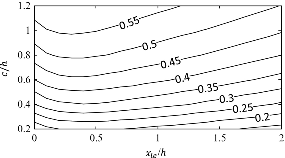
To predict corrections for an open-jet test section usually requires a numerical calculation of some type. Figs. 10.8 through 10.10 show example calculations. Fig. 10.8B is a schematic of a NACA 0012 airfoil in an open jet wind tunnel test section. The airfoil is placed at a geometric angle of attack of 5 degrees in the center of a free jet with its leading edge a distance xle downstream of the nozzle exit of height h. A two-dimensional panel method [8] is used to calculate the flow around the airfoil and the associated deflection of the jet boundaries, these being modeled as surfaces of constant pressure. The best match between the computed airfoil pressure distribution and a parallel free flight calculation is then used to determine the corrected angle of attack and free stream velocity.

Fig. 10.9 shows the corrections to angle of attack, (α′−α)/α′, and free stream velocity ![]() computed as functions of chord length to test section height ratio c/h for a free jet with xle/h=1. Also shown are these corrections computed using a similar method for a closed test section (Fig. 10.8A). In these ratios α and U∞ denote the effective angle of attack and free stream velocity, whereas α′ and
computed as functions of chord length to test section height ratio c/h for a free jet with xle/h=1. Also shown are these corrections computed using a similar method for a closed test section (Fig. 10.8A). In these ratios α and U∞ denote the effective angle of attack and free stream velocity, whereas α′ and ![]() denote the geometric angle of attack and nominal facility free stream. Note that closed test section corrections for airfoils can be accurately estimated analytically using well-established methods [9].
denote the geometric angle of attack and nominal facility free stream. Note that closed test section corrections for airfoils can be accurately estimated analytically using well-established methods [9].

 . Symbols: Δ, closed test section; ○, free-jet test section with xle/h=1; and □, hybrid test section with L/h=2.
The airfoil in the open-jet test section experiences almost no blockage effect (Fig. 10.9B), compared to a correction of a few percent in the closed test section. The interference effect on angle of attack is, however, several times that of the closed test section and, in an absolute sense, very large. For example, an airfoil placed in a free jet requires a correction to angle of attack of over 30% if the chord length is half of the test section width, or larger. Unfortunately, this error is also a function of the positioning of the model relative to the nozzle exit, as shown in Fig. 10.10 where it has been plotted as a function of both xle and c/h. Changing the airfoil profile significantly from a NACA 0012 airfoil section also noticeably affects the correction.
A significant problem with the size of the angle of attack effect is that it can change the character of the flow and thus render the fundamental assumptions of the aerodynamic correction invalid, namely, that the effects of the test flow boundaries are inviscid and in the aerodynamic far field. If this happens, then no effective angle of attack can be found where the pressure distribution resembles that produced in free flight [10]. In such a circumstance there is no other option than to reduce the size of the model relative to the jet or abandon the quantitative relationship of the test to conditions independent of the wind tunnel configuration. Such a test can still be of value, of course, if the goal of the experiment is fundamental scientific insight into phenomena still present in the wind tunnel flow or the validation of a computational method that is used to simulate both the free jet and the model mounted within it.
A third type of configuration used in aeroacoustic testing is the hybrid anechoic tunnel (Fig. 10.11). Here the hard walls of the closed test section are replaced with acoustically transparent walls (termed acoustic windows), generally made from Kevlar fabric. Acoustic instrumentation is placed in an anechoic chamber or chambers external to the acoustic windows. The acoustic windows contain the flow and thus limit the aerodynamic interference, at the same time as enabling sound measurements in the acoustic far field in much the same way as for a free jet.

Fig. 10.11 shows the layout of the hybrid acoustic test section of the Virginia Tech Stability Wind Tunnel [11]. This facility has a square test section 1.83 m on edge. The side walls of the test section consist of 4.21-m long 1.83-m high acoustic windows. Sound generated in the flow passes through these windows into two large anechoic chambers that sit to either side of the test section. The floor and ceiling of the test section include treated flow surfaces designed to minimize acoustic reflections. Fig. 10.12 shows an airfoil model mounted vertically in this test section, as well as a phased microphone array system placed in one of the anechoic chambers to measure the airfoil trailing edge noise. Figs. 10.13 and 10.14 show other implementations of this concept at the 2 m×2 m wind tunnel at the Japan Aerospace Agency (JAXA) in Tokyo, and the Anechoic Flow Facility at the Naval Surface Warfare Center, in Carderock, Maryland. The JAXA facility is configured similarly to the Virginia Tech Stability Tunnel, with the exception that only the starboard-side Kevlar acoustic window is backed by a full anechoic chamber. The comparatively shallow space-saving chamber on the port side serves, primarily, as an acoustic absorber.


The Carderock facility represents a somewhat different arrangement used to contain the 8-foot diameter jet of this otherwise conventional open-jet wind tunnel. The setup shown is for a surface flow noise test on a large model that divides the test section into left and right halves. The facility has an octagonal nozzle necessitating segmented acoustic windows.
The basic idea behind the hybrid configuration is to combine the better features of closed and free-jet test-section configurations for aeroacoustic testing. From the aerodynamic perspective, enclosing the jet in Kevlar walls reduces interference corrections to closed-test section levels. That is not to say that closed-test section methods can be used without modification to estimate corrections, as the porosity and flexibility of the acoustic windows are both significant factors in determining these. Corrections require a test section flow simulation that incorporates these effects. Fig. 10.9 shows example calculations of interference effects for a NACA 0012 airfoil (Fig. 10.8C) computed using an inviscid panel method coupled with a membrane solver and porosity model [11]. Even for large c/h the angle of attack corrections remain small. Free-stream velocity corrections are the same size as those for a closed test section. As evidenced in Fig. 10.15, these corrections are almost independent of the length of the acoustic windows relative to the test section height L/h, for L/h greater than about 2. Note that the angle of attack correction actually passes through zero for c/h≅0.5. This is because there are two contrary influences on this parameter—the porosity of the acoustic windows (which tends to lower angle of attack) and their flexibility (which tends to increase blockage and thus angle of attack). The much lower interference effects compared to a free jet permit testing of substantially larger models, and thus a higher range of Reynolds numbers.

The acoustic windows of a hybrid test section eliminate the need for a jet collector (and eliminate any noise it might generate) and permit a much longer test section compared to its width. Acoustic instrumentation can also be placed much closer to the flow, and thus the sources of interest, than it can be for a jet (Fig. 10.12A). The net effect of these two attributes is that a phased microphone array placed close to the outside of an acoustic window receives sound from a comparatively long stretch of the flow making it easier to distinguish the sounds produced from a model placed at the center of the test section from the parasitic noise sources of the wind tunnel, which appear at the ends of the test section. These acoustic benefits are balanced against the necessity of accounting for acoustic losses for sound transmission through the windows (see Section 10.2.4) and, at frequencies greater than about 15 kHz, the presence of some parasitic noise generated by the flow over the acoustic window material.
10.2 Wind tunnel acoustic corrections
When sound measurements are made in the anechoic chamber surrounding the test section of an open-jet or hybrid anechoic wind tunnel, the sound produced in the flow must cross a shear-layer as it propagates from model to microphone. The shear layer reflects some of the sound and refracts the remainder, bending the otherwise direct path of propagation to the microphone. This changes the amplitude of the sound and its apparent directivity. Some of the amplitude change results from the increased distance traveled by the refracted waves and from the distortion of the wave field produced by the refraction. In a hybrid anechoic tunnel additional amplitude attenuation is produced by the insertion loss of the acoustic window.
We begin by ignoring the shear layer thickness and a possible acoustic window, deferring discussion of these effects to later in this section. Without these complications this situation is amenable to mathematical analysis which provides formulae that can be used to correct sound measurements back to what would have been measured in the absence of the shear layer.
10.2.1 Shear layer refraction
In preparation for addressing this problem, consider a plane sound wave propagating through still air. The wave has a complex pressure amplitude ![]() , a frequency ω and thus a wavenumber, in the direction of propagation, of k=ω/co. The wave will produce a small in-phase velocity fluctuation in the direction of propagation with an amplitude
, a frequency ω and thus a wavenumber, in the direction of propagation, of k=ω/co. The wave will produce a small in-phase velocity fluctuation in the direction of propagation with an amplitude ![]() , referred to as the particle velocity. In terms of the acoustic momentum equation, Eq. (3.3.5), we have
, referred to as the particle velocity. In terms of the acoustic momentum equation, Eq. (3.3.5), we have

and s is distance along the path of propagation. Thus the amplitude of the particle velocity fluctuation is
Now consider plane waves encountering an infinitely thin shear layer, as shown schematically in Fig. 10.16. The shear layer is perpendicular to the x2 direction and separates a uniform flow of velocity U=U∞i in the x1 direction from stationary air. The sound waves incident on the shear layer originate from within the flow and have wavefronts defined by the spherical polar angles θi and ψi. The sound propagates perpendicular to these fronts at speed co at the same time as being swept downstream by the flow at U∞i. A portion of the sound is reflected from the shear layer back into the flow. The reflected sound field has the same form as the incident field except that its component of propagation perpendicular to the shear layer is reversed and thus θr=−θi. The remaining sound is transmitted through the shear layer and appears on the other side as plane wavefronts propagating along the direction defined by the angles θt and ψt. There is no convection on this side of the shear layer.

The relationship between the transmitted, reflected, and incident sound is determined by ensuring that these sound fields are consistent where they meet at the shear layer. The sound waves impose pressure variations on the shear layer and associated out-of-plane motion due to the vertical component of the acoustic particle velocity. These variations take the form of a surface wave that moves across the shear layer tracking the acoustic wavefronts that produce it. The reflection mechanism requires that the incident and reflected waves be in phase at the shear layer. The transmitted and incident/reflected waves must also be in phase here, since otherwise there would be no way for the pressure and surface motions to be consistent across the shear layer.
First we will match the velocity of propagation of the surface wave with the transmitted sound wave. The transmitted sound wave propagates at the sound speed co, and the distance between successive wavefronts in the direction of propagation is the wavelength λ. Since the direction of propagation makes an angle θt to the shear layer, the distance between the wavefronts where they meet with the shear layer is λs=λ/cos θt. The surface wave must therefore travel at a speed Us=co/cos θt to match the propagation of the transmitted sound, and thus the velocity of the surface wave expressed in terms of components in the x1 and x3 directions is
For the incident wave we must also add the convection by the mean flow and so, in terms of the incident wave angles,

We see that the surface wave speed can also be expressed as Us=co/cos θt+U∞cos ψi. Matching components in Eqs. (10.2.3), (10.2.4), we have
and

where M=U∞/co. Solving these equations gives the angles of the transmitted sound wave in terms of those of the incident sound wave

and, conversely, for the angles of the incident sound wave

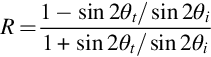
These equations constitute Snell's law for shear layer refraction. To determine the amplitude of the transmitted sound compared to the incident we use the fact that the pressure fluctuations and deflections of the shear layer implied by the incident and reflected wave must be consistent with those implied by the transmitted wave. Using subscripts “i,” “r,” and “t” to denote incident, reflected, and transmitted we have that, for the pressure,

where k=ω/c∞, x2=h identifies the shear layer, and we have matched the wavenumbers at the shear-layer interface. At the interface the pressure must match so
and thus C=A+B. Defining the reflection and transmission coefficients as ![]() and
and ![]() Eq. (10.2.9) becomes
Eq. (10.2.9) becomes
We must also consider the displacement of the shear layer ξ normal to the flow associated with the surface wave. For a harmonic sound wave, the displacement of the shear layer will be sinusoidal and have the form
This must match the acoustic particle velocity on either side of the layer in the x2 direction. In the stationary air outside the flow we have, from Eq. (10.2.2),

Inside the flow, the sound wave is being convected at speed U∞, and so we must use the convective derivative to get the displacement velocity. We also have to account for the fact that the acoustic particle velocity of the reflected wave is reversed compared to that of the incident wave. Thus the displacement velocity is,

so

Using Snell's law (Eq. 10.2.8) and combining the above expressions to eliminate D gives
Dividing through by A to evaluate R and T, we obtain,
which in combination with Eq. (10.2.10) implies

and
Eqs. (10.2.14), (10.2.15), along with Eqs. (10.2.7), (10.2.8), first derived in two-dimensions by Ribner [12], completely define refraction effects for the case of a thin shear layer. These expressions have been derived for plane waves and a flat shear layer. However, they can equally well be taken to represent arbitrarily small portions of a nonplanar sound field or curved shear layer, and thus the results can also be applied locally to much more general situations. Exactly how the above relations are employed to correct measured noise data will depend on the specifics of an experimental setup.
10.2.2 Corrections for a two-dimensional planar jet
Consider the arrangement shown in Fig. 10.17. The figure shows an acoustic source at location S in a wind tunnel flow of velocity U∞ located a distance h inside the shear layer. The sound is being measured at location M, outside the shear layer at a distance and angle rm and θm from the source. Because of refraction, the measured sound arrives indirectly at M via the point R. Note that the angles θi and θt in Fig. 10.17 correspond to those in Fig. 10.16. The plane of the shear layer is perpendicular to the plane MRS. We wish to correct the measurement for the effects of the shear layer. In other words, we wish to know the true directivity angle θc (which also gives the corrected observer distance rc=H/sin θc), the amplitude of the acoustic pressure ![]() that would have been measured at point C if the flow had been unbounded, and the difference in the corresponding arrival time of the sound waves τm−τc. We need to know these in terms of θm and the measured pressure amplitude
that would have been measured at point C if the flow had been unbounded, and the difference in the corresponding arrival time of the sound waves τm−τc. We need to know these in terms of θm and the measured pressure amplitude ![]() and the geometrical parameters h and H.
and the geometrical parameters h and H.

To obtain the true directivity angle θc we note first that
To eliminate θt we first use Snell's law (Eq. 10.2.7) for ψi=0 to give

Next, we relate θi and θc using the kinematics of the sound propagation in the flow. Consider the point S′ (Fig. 10.17) located at the apparent center of the spherical wave arriving at point R on the shear layer. The time taken for this wave to propagate to R from the source is h/(cosin θi), and in this time its center has convected downstream a distance hM/sin θi between S and S′. We therefore have
which is solved using tangent half-angle identities to give,
Eqs. (10.2.19), (10.2.17), (10.2.16) are simple to evaluate analytically in reverse, i.e., to determine θm from θc given M and h/H. An iterative method is needed to determine θc from θm. For these calculations it is useful to rearrange Eq. (10.2.17) as
where the square root takes the sign of sec θi. Simpler relationships exist for limiting cases. In the limit of H/h→∞, θm=θt and the relationship becomes

and, as H/h→1 we simply recover that θc=θm.
The correction to the receiving angle is plotted as a function of Mach number in Fig. 10.18A for H/h=2. Corrections become particularly large in the forward arc and as the Mach number is increased. However, for M≤0.2 they are less than 10 degrees and roughly constant with θm over the central portion of the arc between θm of 45 and 135 degrees where most measurements are made. Fig. 10.18B shows the same correction plotted as a function of H/h for M=0.2. The correction increases with increasing distance of the observer from the flow. Eq. (10.2.20) representing the limit H/h→∞ only serves as an accurate approximation for H/h greater than about 5.

With θc determined, the difference in the time of arrival of the measured signal at M and its hypothetical arrival across the flow at C is given by differencing the propagation times from point R

where θt and θi can be determined from Eqs. (10.2.16), (10.2.17).
To determine ![]() we must account for both the loss of pressure amplitude in transmission through the shear layer (Eq. 10.2.14) and the difference in the spreading of the sound field between R and M as compared to R and C. In the absence of the shear layer the acoustic wave-fronts remain spherical, and so the square of the pressure amplitude is inversely proportional to the square of the propagation distance from the source, i.e.,
we must account for both the loss of pressure amplitude in transmission through the shear layer (Eq. 10.2.14) and the difference in the spreading of the sound field between R and M as compared to R and C. In the absence of the shear layer the acoustic wave-fronts remain spherical, and so the square of the pressure amplitude is inversely proportional to the square of the propagation distance from the source, i.e.,

Where, consistent with the Snell's law analysis above, we are using ![]() and
and ![]() to denote the amplitude of the incident and transmitted sound pressure for the shear layer at R, respectively. Determining
to denote the amplitude of the incident and transmitted sound pressure for the shear layer at R, respectively. Determining ![]() is more involved because we must account for the change in the spreading that occurs with refraction. Fig. 10.19 illustrates the method. We consider the sound passing through an elemental area dx1dx3 at R expanding out the area dx′1dx′3 at M. From Fig. 10.19,
is more involved because we must account for the change in the spreading that occurs with refraction. Fig. 10.19 illustrates the method. We consider the sound passing through an elemental area dx1dx3 at R expanding out the area dx′1dx′3 at M. From Fig. 10.19,


Note that dθt as drawn in Fig. 10.19 is negative, resulting in the minus sign that appears inside the first bracket. Since the square of the sound pressure varies inversely with the cross-sectional area, and since the elemental areas at R and M make equal angles to the ray RM, then

where the derivatives are evaluated at R. To determine the derivatives of θt and ψt, we first consider position where a general sound ray (i.e., one not confined to the x1 x2 plane) passes through the shear layer in terms of θi and ψi, Fig. 10.20, which is


Differentiating these expressions with respect to θi and ψi, differentiating Snell's law for these angles (Eq. 10.2.8) with respect to θt and ψt, using the chain rule, and evaluating for ψt=0 give


where ζ2≡(1−M cos θt)2−cos2 θt. Since the same process yields ∂x3/∂θt=∂x1/∂ψt=0, the derivatives of θt and ψt needed for Eq. (10.2.24) are simply the reciprocals of Eqs. (10.2.26), (10.2.27), and thus
Finally, from Eqs. (10.2.28), (10.2.22), (10.2.14) we obtain

which can be rewritten as

This amplitude correction is plotted in Fig. 10.21A as a function of the angle of the sound measurement θm and Mach number for H/h=2. Over much of the rearward arc ![]() is <1 (i.e., negative in terms of dB), primarily because the shear layer transmission coefficient T is greater than1 here. Over the forward arc, however, the spreading effect dominates making the corrected pressure amplitude significantly greater than that measured, particularly as the Mach number is increased above 0.2. Increasing the distance of the microphone from the shear layer, i.e., increasing H/h, tends to magnify the corrections as shown for M=0.2 in Fig. 10.21B. At Mach numbers of 0.3 and less, microphone measurements made close to θm=90 degrees require no significant amplitude correction. In interpreting Figs. 10.18 and 10.21, it is important to note that space limitations and the extent of the flow often constrain acoustic measurements to directivity angles between θm of 45 and 135 degrees. Note that Eq. (10.2.30) and the directivity corrections introduced starting at Eq. (10.2.16) were first derived by Amiet [13,14].
is <1 (i.e., negative in terms of dB), primarily because the shear layer transmission coefficient T is greater than1 here. Over the forward arc, however, the spreading effect dominates making the corrected pressure amplitude significantly greater than that measured, particularly as the Mach number is increased above 0.2. Increasing the distance of the microphone from the shear layer, i.e., increasing H/h, tends to magnify the corrections as shown for M=0.2 in Fig. 10.21B. At Mach numbers of 0.3 and less, microphone measurements made close to θm=90 degrees require no significant amplitude correction. In interpreting Figs. 10.18 and 10.21, it is important to note that space limitations and the extent of the flow often constrain acoustic measurements to directivity angles between θm of 45 and 135 degrees. Note that Eq. (10.2.30) and the directivity corrections introduced starting at Eq. (10.2.16) were first derived by Amiet [13,14].

The results of the above analysis allow for two important physical observations concerning the refraction phenomenon that we have not yet commented on. First, for incident wave angles θi sufficiently close to 180 degrees (i.e., directed toward the oncoming flow), the sound can suffer total internal reflection and no transmitted wave is produced. In this situation the magnitude of the right hand side of Eq. (10.2.7) is >1 so that there is no solution for θt. Indeed, we can infer from this expression that for transmission to occur we must have

Fig. 10.22 shows this bound plotted as a function of Mach number, total internal reflection occurring for angles to the right of the lines drawn. The effect clearly grows with Mach number, but even for a Mach number of 0.15 it is not possible to receive sound outside the flow propagating into the wind, closer than 30 degrees from the oncoming flow direction. This may be a more significant concern for hybrid anechoic tunnels since it is more feasible to place instrumentation close to the shear layer in this configuration.

A second observation becomes apparent when Eq. (10.2.17) in combination with the trigonometry apparent in Fig. 10.17 is used to plot the wavefronts of sound propagating through a shear layer from a point source, as has been done in Fig. 10.23. Here the sound source is located at the origin. The refracted wavefronts are clearly noncircular (or nonspherical in the three-dimensional view), and their asymmetry becomes more pronounced as they propagate further from the shear layer. This means that there is no virtual image location for the sound. Thus if, as discussed in Chapter 12, we were to use a microphone phased array to construct an image of the source from the diffracted sound, then that image will be blurred unless we account for the wavefront distortion using, for example, the propagation time correction of Eq. (10.2.21).

10.2.3 Effects of shear layer thickness and curvature
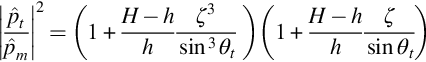
The effects of shear layer thickness are discussed by Amiet [13,14], through comparison of measured corrections with the predictions made by the above formulae. He argues that shear-layer thickness effects are generally most significant for emission angles closest to those producing total internal reflection and thus are not often important in measurements. Additionally, Amiet [14] argues that Eq. (10.2.30) will still apply in the limit of a thick shear layer, with the exception that there will be no loss of acoustic energy in the shear layer since no reflected wave is produced. This has the effect of multiplying the measured pressure amplitude by the factor (1−R2)−1/2, which, using Eqs. (10.2.15), (10.2.17), can be rewritten as

Amiet [14] also gives results that incorporate the effects of shear layer curvature, as in the round shear layer formed around a circular free jet.
10.2.4 Considerations for hybrid anechoic tunnels
In hybrid anechoic wind tunnels the Kevlar acoustic windows used to contain the flow produce an attenuation of the sound additional to that associated with refraction. Otherwise, the effects of refraction are expected to be identical to those derived in Sections 10.2.1 and 10.2.2. Indeed, the presence of the Kevlar results in a much thinner and flatter shear layer than will be realized in most open-jet tunnel situations, and so some of the assumptions of the analysis are more accurate. Snell's law (Eqs. 10.2.7, 10.2.8) and the geometric relations derived in Eqs. (10.2.16)–(10.2.28) all apply. The transmission and reflection result (Eqs. 10.2.14, 10.2.15) and the pressure amplitude result that depends on it (Eq. 10.2.30), however, need to be modified to account for the insertion loss associated with the Kevlar barrier. Note that losses in transmission through an acoustic window do not usually impact the signal-to-noise ratio of a sound measurement, since both signal and the parasitic noise of the facility must pass through the Kevlar and are thus attenuated by the same amount.
The attenuation produced by the Kevlar depends not only on its physical characteristics (porosity and flexibility) but also on the speed of the flow that it is exposed to. This is because the flow influences the characteristics of the motion through the pores and the movement of the fabric that couples the sound waves on the incident and transmitted sides. Fortunately, such losses can be quite easily measured using, for example, the setup shown in Fig. 10.24.

A speaker and a microphone are positioned facing each other across the empty test section. Both are mounted in anechoic chamber areas outside the test section, and thus the sound from the speaker must traverse both Kevlar windows and the flow in the test section to be recorded by the microphone. The sound attenuation between the speaker and microphone, as compared to that which would occur in a free-field environment, reveals the insertion loss associated with traversing two acoustic windows subject to flow. The loss associated with a single window, that is needed to adjust far-field noise measurements of a source in the test section, is simply half of this value when expressed in decibels. Measuring the attenuation associated with transmission through both windows and shear layers avoids the problems associated with placing speakers or microphones in the flow.
Most hybrid wind tunnels to date have used Kevlar 120 scrim as the acoustic window material. This fabric weighs 58 g/m2 and has a plain weave with 34 threads per inch in both directions made from Kevlar 49 fiber. Insertion losses associated with one batch of this material [11], measured using the method depicted in Fig. 10.24, and then curve fitted are shown in Fig. 10.25. The curve fits are given by the expressions:

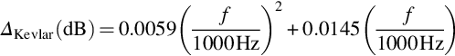
representing the transmission loss through the Kevlar with no flow, and
for the additional flow-related losses. As can be seen in Fig. 10.25, the total correction needed for the presence of the Kevlar (ΔKevlar+ΔFlow) increases with both frequency and flow speed. While Fig. 10.25 and Eqs. (10.2.33), (10.2.34) are perhaps useful in general for providing rough estimates of Kevlar losses to be used in experiment or facility design, a measured calibration specific to the acoustic windows used in a particular test or facility is important for measurement accuracy. Different batches of the same material made to identical specifications can differ sufficiently (e.g., in porosity) to have a significant impact upon loss characteristics.
10.3 Sound measurement
Sound measurements at conditions likely to be generated by low Mach number flows are commonly made using condenser microphones—microphones that use the change in capacitance between a membrane and a backing plate. The membrane vibrates in response to the sound, and the capacitance changes as the distance between the membrane and the backing plate fluctuates as a function of time. Conventional condenser microphones require a power source to maintain a charge across the membrane and the backing plate, so a change in capacitance appears as a change in voltage. In electret microphones either the diaphragm or the fixed plate of the capacitor is made from a ferro-electric material that carries a permanent electric charge (referred to as prepolarized). This eliminates the need for a voltage source for the microphone, though power is usually still required because an integrated preamplifier is commonly part of these devices.
Instrumentation microphones designed for scientific work are often the most expensive but can provide well-defined, accurately documented, and stable characteristics. Examples are the 1/2-in. diameter B&K 4190 illustrated in Fig. 10.26A and the 1/4-in. G.R.A.S. 40-PH-S5-1 shown in Fig. 10.26B. Microphones of this type may be provided with documentation of their frequency response when exposed to plane sound waves parallel to the diaphragm, as well as deviations from that response for off-axis sound (e.g., Fig. 10.27). Within its operating range (6.3 Hz–20 kHz for the B&K 4190) this type of microphone will generally have an almost constant amplitude response to sources ahead of the diaphragm so that in this range only a single value of the microphone sensitivity is needed to make a quantitative sound measurement. Precise measurement of this sensitivity (to account for environmental conditions at the time of a measurement) can be made using a pistonphone. This is a handheld device produces pressure fluctuations of known amplitude by using the mechanical motion of a vibrating piston at a fixed frequency to simulate a sound wave by compressing a fixed volume of air to which the microphone diaphragm is exposed.

Instrumentation microphones come in a range of diameters. Large diameter microphones (e.g., 1/2 or 1 in.) are more sensitive to acoustic pressure fluctuations because those fluctuations are integrated over a larger diaphragm area. Such microphones are useful for measuring sources that are particularly quiet at laboratory scale, such as roughness noise, where good electrical signal-to-noise ratio is needed. At the same time, the larger diaphragm has greater inertia limiting the frequency response. While suffering from lower sensitivity, smaller diameter microphones (e.g., 1/4 and 1/8 in.) may have a greater range, both in terms of the intensity of the sound and the frequencies they can measure. For example, the B&K model 4138 1/8 in. microphone pictured in Fig. 10.26C can measure sounds up to 168 dB and 140 kHz.
The size of the diaphragm is also important compared to the wavelength of the sound. When the wavelength becomes comparable to the diameter then the scattering of the sound field around the end of the microphone and the spatial distribution of the diaphragm sensitivity become important in determining the response. Fig. 10.27 shows, for example, the deviations in the response of the B&K 4190 with the direction of the incident sound. This microphone has a 1/2-in. diaphragm, and we see that the directionality of the sound becomes a substantial factor at around 6 kHz, where the quarter wavelength is approximately equal to the diaphragm diameter. At 20 kHz, the microphone is 10 dB less sensitive to sound directed at the side of the microphone, or from behind, than it is to sound originating from in front. Instrumentation microphones are usually designated as free-field microphones (like the B&K model 4190), optimized as far as possible to measure sound incident on the microphone from any direction, or pressure-field microphones designed to measure sound (or fluid dynamic pressure fluctuations) at a wall. Pressure-field microphones, such as the B&K model 4138 in Fig. 10.26C, usually include a vent designed to equalize the mean pressure on the two sides of the microphone for situations where the face of the microphone is exposed to a pressure significantly different from ambient.
At the lower end of the cost spectrum are devices designed for mass market applications such as lavalier microphones, cell-phones, hearing aids, and units designed for the recording and performance industry. Many of these devices are electret microphones, and a subset can be used for sound measurement in low Mach number applications as long as the experimentalist is willing to take the time to select and calibrate these sensors to the precision needed for scientific work. It is common practice to perform frequency response calibrations of such microphones using an instrumentation microphone as a reference, by subjecting both microphones to a broadband sound field generated by a loud speaker. Such a calibration needs to be done in an environment with a well-defined acoustic character, such as a sealed cavity, a pipe, or an anechoic chamber. Consistent placement and configuration of the test and reference microphones is usually critical to ensure that they are exposed to exactly the same sound field. Examples of such microphones include the Sennheiser KE 4-211-2 shown in Fig. 10.26D and the Panasonic WM-64PNT of Fig. 10.26E. Stability, low noise, and adequate amplitude and frequency range are important considerations in selecting a low-cost microphone for an aeroacoustic test. For situations where multiple microphones are to be used as part of a system (such as a phased microphone array) measuring and matching the phase calibrations of the microphones are often crucial.
The placement and mounting of microphones outside of the test flow involves a number of considerations. It is usually desirable for the microphone to be as close as possible to the source to maximize signal-to-noise ratio. At the same time, keeping the microphone in the acoustic far field (at least one wavelength from the source) is often desirable to simplify the interpretation of the measurement. Also, placing the microphone too close to the free jet or acoustic window can result in contamination by near-field pressure fluctuations associated with the turbulent shear layer. It is usual to orient the microphone to point as directly as possible at the source. This aligns the wavefronts parallel to the diaphragm and makes use of the most favorable microphone response. To exploit the best characteristics of the anechoic chamber, microphones are usually placed at least a quarter wavelength away from the walls, defined by the wedge tips. To avoid unpredictable scattering effects microphones should either use slender mounts and be held from behind or be mounted on a solid surface designed to cleanly reflect the incoming acoustic waves (in which case the measured sound pressure amplitude is doubled because of the addition of the incident and reflected waves). Fig. 10.28 shows single microphones mounted with these considerations in mind in an open-jet wind tunnel. Note that acoustic foam is wrapped around the support beams of the microphone gantry in order to reduce acoustic reflections. Two different mounting strategies for a microphone array are shown in Figs. 10.29 and 10.30. In Fig. 10.29 the microphones are mounted flush in the face of a circular carbon fiber disk designed to reflect the sound, and in Fig. 10.30 the microphones are supported from behind using an open lattice designed to transmit the sound at wavelengths of interest.


It is often of interest to obtain sound measurements at angles that require placing microphones inside the flow. A good example here is rotor testing, where sound radiated on or near the rotor axis is of particular scientific interest. When a microphone is placed directly in the flow its signal will be contaminated with turbulent and sound pressure fluctuations resulting from the interaction of the microphone and its support with the flow. To minimize the contamination an aerodynamic fore-body is used with the microphone, and a streamlined fairing is placed over the supporting strut. The typical microphone fairing shown in Fig. 10.31 is a 1/2-in. diameter B&K model UA 0386 nose cone. This consists of a bullet-shaped housing with a circumferential opening covered by a porous screen. When mounted to the front of a microphone the space interior to the screen forms a cylindrical cavity with one face formed by the microphone diaphragm. Regardless of the orientation of the acoustic source of interest, the microphone is mounted with the nose-cone facing directly into the flow. In this position its streamlined shape minimizes the generation of turbulence, and the screen keeps any flow generated pressure fluctuations separated from the diaphragm. Furthermore, the screen tends to average out turbulent pressure fluctuations that are incoherent around its circumference. The principal drawback of this arrangement is that the nose cone changes the response of the microphone to sound at wavelengths of comparable size. Fig. 10.27 shows the effect of this nose cone on the free-field response of the 1/2-in. B&K 4190 microphone. For sound waves directed roughly at the face of the microphone θ=0 degrees and 30 degrees the nose cone considerably attenuates the intensity of the sound measured at frequencies above about 15 kHz. The forebody actually amplifies sound coming from the side and behind in this frequency range. Obviously, these effects need to be corrected if sound at these frequencies is to be measured accurately. Note that other longer forebody designs can further reduce flow noise contamination [15].

The design of the strut supporting the microphone in the flow is equally critical. Even as a streamlined airfoil, the strut will be an acoustic source that competes with the sound produced by the model under test. Making the strut as quiet as possible, maximizing the distance of the microphone from the strut (by using a long sting support) can be simple and effective measures. (Note that Fig. 10.31 shows a microphone being used to measure relatively intense sound from a rotor system, and thus a short microphone sting was adequate in this case.) Ideally, the airfoil section chosen for the strut needs to be quiet. In particular, it must not generate vortex shedding tones while being thick enough to provide rigid structural support for the microphone. The McMasters-Henderson airfoil [16], a symmetric 28% thick section illustrated in Fig. 10.32, works well in this role [15].

10.4 The measurement of turbulent pressure fluctuations
Microphones respond to pressure fluctuations regardless of whether those fluctuations arise from sound waves or flow features. The same basic devices are thus used for measuring the fluid dynamic pressure fluctuations at a surface immersed in a turbulent flow. Such pressure fluctuations are often of interest since they represent an acoustic source (through Curle's equation) or because they help reveal the physical characteristics of a turbulent flow that is otherwise responsible for the aerodynamic noise produced.
The requirements of fluid dynamic pressure fluctuation measurements are quite different from those of sound measurements, and thus the details of the devices used, and how they are used, can be significantly different. The considerations that lead to these requirements concern the scale, intensity, and the location of the pressure fluctuations.
At low Mach number the scale of the turbulent eddies L in a flow is much smaller than the wavelength of the sound they might produce λ, the ratio being roughly the Mach number. (This is because we expect the passing frequency of the eddies U/L to be the same as the frequency of the sound co/λ.) Suppose, for example, we are concerned with characterizing the pressure fluctuations underneath a turbulent boundary layer on the surface of an airfoil. Such pressure fluctuations define the basic source terms for trailing edge noise and roughness noise to be discussed in Chapter 15. As discussed in Section 9.2.3 and shown in Fig. 9.20B the highest frequency pressure fluctuations in the boundary layer occur at a normalized angular frequency of about ων/uτ2. The friction velocity uτ is expected to be about 5% of the free stream U∞, so for an airfoil traveling through air at 50 m/s, ω≅4.3×10⁵ or 68 kHz assuming sea-level conditions. If we take the convection velocity of the smallest eddies to be 0.6U∞ (Fig. 9.19), then this implies that these eddies are a little under half a millimeter in size. If we are interested in completely resolving the pointwise pressure, then we must be able to resolve pressure scales at least this small. This is a major challenge. Studies using different size transducers [17] have shown that the measurement of the pressure spectrum becomes independent of transducer size when the effective transducer diameter, normalized on the inner boundary layer variables as d+=duτ/ν, is less than about 18. For the airfoil example, this implies a diameter d, of only 0.1 mm. In most cases it is not possible to meet this requirement—sufficiently small transducers simply do not exist. However, making the effective transducer size small is still important in minimizing the underresolution if we are interested in characterizing the pressure at a point. In doing so it usually makes sense to match the dynamic response of the microphone and its spatial response. If we need to use a transducer to measure the pressure fluctuations on our airfoil which has a dynamic response that dies off above 17 kHz, say, then there is no real purpose for its effective diameter to be less than about 0.4 mm.
At low Mach numbers, the intensity of pressure fluctuations in a turbulent flow is usually many orders of magnitude larger than the far-field sound the flow produces. Transducer dynamic range is therefore a consideration. In an equilibrium turbulent boundary layer the root-mean-square pressure fluctuation at the wall is about 1% of the free stream dynamic pressure ![]() and approximately three times the wall shear stress τw, corresponding to 20 Pa or 120 dB (relative to 20 μPa) in the above airfoil example. If it were produced by sound waves, a level of 120 dB would be close to the threshold of pain and thus is already near the upper limit of many commercially available microphones. Furthermore, simple perturbations to the boundary layer, such as produced by a step in the surface, can increase the RMS pressure fluctuation by more than an order of magnitude, meaning that a transducer with a 140 dB range would be inadequate in this case. One benefit of the high range of aerodynamic pressure fluctuations is that it does permit the use of solid-state transducers that are normally too insensitive for sound measurement. Such transducers are usually piezo-resistive (electrical resistance proportional to pressure) or piezo electric (charge proportional to pressure).
and approximately three times the wall shear stress τw, corresponding to 20 Pa or 120 dB (relative to 20 μPa) in the above airfoil example. If it were produced by sound waves, a level of 120 dB would be close to the threshold of pain and thus is already near the upper limit of many commercially available microphones. Furthermore, simple perturbations to the boundary layer, such as produced by a step in the surface, can increase the RMS pressure fluctuation by more than an order of magnitude, meaning that a transducer with a 140 dB range would be inadequate in this case. One benefit of the high range of aerodynamic pressure fluctuations is that it does permit the use of solid-state transducers that are normally too insensitive for sound measurement. Such transducers are usually piezo-resistive (electrical resistance proportional to pressure) or piezo electric (charge proportional to pressure).
The final factor in the selection of pressure transducers for flow measurement is the space available. In some applications this may be the dominant constraint. Trailing edge noise is again a convenient example. The radiated noise is nominally dependent on the surface pressure fluctuation difference between the two sides of the airfoil at the trailing edge itself. There is therefore a desire to measure as close as possible to this point so that the measured characteristics are accurately representative of the source term. Consider the commonly used NACA 0012 airfoil, for example. At a point 5% of the chord length c upstream of the trailing edge (a reasonable place for a trailing edge pressure measurement), this airfoil has a thickness equivalent to 1.4% c. For a half-meter chord length model this implies 7 mm thickness to accommodate one or two surface pressure sensors (if the difference is being measured) and their wiring.
Fig. 10.33 shows some examples of microphones suitable for turbulent pressure fluctuation measurement at low Mach number. We use these examples to illustrate the typical trade-offs made in selecting suitable transducers, rather than recommending any specific device. The two electret microphones, the Knowles FG-23742 and the Sennheiser KE-4-211-2, are supplied with fairly small openings (0.75 and 1 mm diameter, respectively) and thus have an inherent spatial resolution that may be sufficient for some applications. These microphones are quite sensitive (6.7 and 10 mV/Pa, respectively) implying measurements relatively free of electrical noise, have a useful frequency response (to 10 and 20 kHz), and are compact enough for installation within a confined space (particularly the Knowles for which the casing is only 2.5 mm in diameter and depth). On the other side, these devices have limited dynamic ranges of about 115 dB for the Knowles and 140 dB (with some distortion) for the Sennheiser. Much higher ranges can be achieved using the solid-state Kulite LQ-062-5D and the Endevco 8514-10 both of which have pressure fluctuation ranges that exceed 170 dB, have frequency response characteristics from DC to over 100 kHz, and come in relatively compact packages with effective sensor diameters of approximately 0.7 and 1.7 mm, respectively. The caveat here is that the large range implies a low sensitivity, of about 4 and 3 μV/Pa.

A different option is to use a small instrumentation microphone, such as the 1/8-in. B&K 4138 pictured in Fig. 10.33A. This microphone combines a range (168 dB) and sensitivity (1 mV/Pa) that are well suited to most low Mach number flows. If device size is not a limitation, then the dominant shortcoming of this transducer is the large diameter of its diaphragm (3 mm). A simple and common way to improve the spatial resolution of microphones of this type is to place a pinhole over the diaphragm (compare Figs. 10.33A and 10.26C). However, it is important to recognize and account for the fact that this substantially impacts the frequency response.
The cavity and pinhole aperture above the microphone together form what is known as a Helmholtz resonator as shown in Fig. 10.34. As long as the dimensions of the cavity and pinhole are small compared to the acoustic wavelength, then the pressure sensed in the cavity by the microphone pm can be determined from the pressure experienced at the top of the pinhole p using a one-dimensional momentum balance. The rate of change of momentum of the fluid oscillating through the pinhole is generated by the pressure difference between the cavity and the ambient (pm−p) acting over the pinhole area A. This is opposed by the frictional resistance to flow through the pinhole which we will assume is proportional to the flow velocity with a damping coefficient RA, where R is the termed the acoustic resistance. Thus,


Here M is the mass of fluid in motion and u2 is its velocity. Assuming harmonic fluctuations, i.e., u2, p, and pm are given by their amplitudes ![]() and
and ![]() multiplied by exp(−iωt), this becomes
multiplied by exp(−iωt), this becomes
The movement of the flow out of the pinhole produces a rate of change of the density of the air in the cavity, given by the associated mass flow rate and the cavity volume

where this has been equated to the pressure in the cavity pm assuming isentropic compression. In terms of amplitudes this relationship can be rewritten as

Substituting into Eq. (10.4.2) and rearranging we obtain

We see that the pinhole cavity behaves as a simple second-order system with a stiffness given by ρocoA2/V. The mass of the fluid in motion M can be computed from the product of the air density, the pinhole area, and an effective pinhole depth Leff. This is generally different from the physical depth L to account for the additional fluid just above and below the pinhole aperture that is involved in the motion.
The appropriate values for Leff and R are dependent upon the specifics of the situation. With no mean motion in the ambient and a circular pinhole that is shallow compared to its diameter d, potential flow modeling [18] indicates that Leff=πd/4. When the pinhole depth is significant this estimate can be modified to
Different formulas for the acoustic resistance exist, a common one being [19]
where ν is the kinematic viscosity of the air. Behaving as a second-order system the response of the cavity ![]() will have a natural frequency
will have a natural frequency

where D denotes the microphone diaphragm diameter and h the distance between the diaphragm and the bottom of the pinhole. Obviously maximizing the frequency response means minimizing the depth of the diaphragm below the surface, given a fixed microphone and pinhole diameter. The amplitude response at the natural frequency is

using the resistance formula of Eq. (10.4.7). The measured response function of the B&K 4138 microphone with half-millimeter diameter pinhole pictured in Fig. 10.33A as shown in Fig. 10.35. Using known geometry (D=3.2 mm, d=0.5 mm) and environmental conditions (co=340 m/s, ν=1.6×10⁻⁵ m2/s) and taking h and L to be 0.5 and 0.2 mm, respectively, Eqs. (10.4.8), (10.4.9) give a natural frequency of 16.6 kHz and an amplitude response at this frequency of 21 dB. While the predicted natural frequency appears accurate, the amplitude is not, reflecting the fact that the resistance formula of Eq. (10.4.7) is quite uncertain. In particular, when using a microphone with pinhole to measure the fluctuating pressure under a flow, one would expect shear flow over the top of the pinhole to have a substantial effect on the acoustic resistance. Past measurements have indicated both an increase [19] and a decrease [20] in effective resistance in the presence of a grazing flow, in different circumstances.

Overall, the important observation here is that enhancing the spatial resolution of a microphone using a pinhole has a substantial effect on its dynamic response that is likely to impact the frequency range of interest in most low Mach number flows. Given the magnitude of the effects, and the uncertainties in their theoretical estimation, dynamic calibration of the microphone with pinhole is essential. This is often done by comparing the output with that of an unmodified instrumentation microphone when both are exposed to a broadband acoustic source.
Resolving the pointwise pressure is not always the goal of a surface pressure measurement in a flow. Sometimes we are interested in deliberate spatial averaging of the surface pressure fluctuations, typically if we are interested in revealing the portion of the pressure field that is directly related to the near-field of an acoustic response. For example, if we are considering the response of an airfoil in turbulence and the leading edge noise it produces (e.g., Fig. 8.2), then at low Mach number the source term is characterized by the zero spanwise wavenumber component of the surface pressure fluctuation (i.e., its spanwise average) produced on the airfoil leading edge by the incident turbulence. Likewise, at low Mach number the sound produced by flow over a step is determined by the unsteady force on the step faces and thus the spatially averaged pressures there. Fig. 10.36 shows a linear array of 24 half-inch microphones developed precisely for this application. The microphones are used with their diaphragms exposed and mounted flush with the surface, so as not to disturb the flow and to take advantage of the averaging of the pressure fluctuations over each diaphragm as well as the array as a whole.

The spatial sensitivity distribution of an instrumentation microphone diaphragm was measured by Brüel and Rasmussen [22] and can be predicted by the function [23,24]

where α=2.675, Jo denotes the Bessel function of the first kind of zero order, r is the distance from the center of the microphone, and rmax is the diaphragm radius. This function, plotted in Fig. 10.37, shows how the microphone is less sensitive at its edges and thus has somewhat narrower spatial resolution than implied by its physical diameter.
The challenge with this type of measurement system is in establishing the extent to which the array produces an acceptable approximation to the ideal intended result (usually defined by a parallel aeroacoustic analysis). For the array of Fig. 10.36 the ideal result was the uniform averaging of the pressure over an infinitely extending spanwise strip. One way this can be done when the turbulence is generated by a boundary-layer like flow is to exploit the models for the wave-number frequency spectrum of the wall pressure Φpp(k1,k3,ω) introduced at the end of Chapter 9. Specifically, given the sensitivity distribution of each microphone, any array result can be written as a wavenumber filter function F(k1,k3). In our example, this is obtained by Fourier transforming the sum of the 24 spanwise distributed microphone response functions representing the spatial sensitivity map of the array. The model spectrum (scaled according to boundary layer parameters appropriate to the experiment) is then integrated, weighted by this filter, to estimate the frequency spectrum of the array output, i.e.,

This can then be compared to the same integration carried out using a filter function FI(k1,k3) representing the ideal intended measurement GppI(ω). By comparing Gpp(ω) and GppI(ω) the frequency range within which the measurement is likely to be accurate can be inferred.
10.5 Velocity measurement
Measuring the velocity field of a flow is often a central component of aeroacoustics experiments. First, velocity measurements are needed to quantitatively reveal the form of the flow in which the noise is being produced. An example here would be measuring mean flow field around an airfoil that is a source of trailing edge noise. Such measurements would reveal the thickness of the boundary layer and the velocity distribution within it—important contextual and scaling information for the noise produced. Second, velocity measurements are often made to directly quantify the acoustic source, such as measuring the upwash fluctuations produced by turbulence approaching a noise-producing leading edge. In this section we focus our discussion on instrumentation suitable for this second purpose and the associated issues. For a more general review of instrumentation for aerodynamic velocity and turbulence measurements the reader is referred to a dedicated text such as Tropea et al. [25].
Hot-wire anemometry serves as a basic tool in many aeroacoustics experiments. Hot wires provide continuous measurement of the fluctuating velocity at a fixed point as in a flow as turbulence is convected past, in much the same way that a noise generating device experiences the turbulence. The fluctuating signals generated by a hot-wire probe can be readily analyzed to determine velocity spectra and, if pairs of probes are used, space time correlations. These are capabilities that match well with the scientific challenge of characterizing sound generated as a result of interaction with the turbulence. Hot-wire anemometry is long established technology that is well understood. One of its drawbacks is that it can only be used accurately in regions where the turbulent fluctuations are significantly smaller than the mean velocity and thus is restricted to flows outside regions of separated flow. A second limitation is that it is intrusive, requiring introduction of a solid probe to the flow. In most unseparated flows, it is possible to arrange the mounting of probes so that the introduction of the hot wire does not significantly disturb the flow at the measurement point. However, it is almost inevitable that any probe arrangement will generate significant sound or otherwise disturb the aeroacoustic interaction under study. Hot-wire measurements therefore cannot usually be made simultaneously with acoustic measurements, and duplicate runs of an experiment are usually required to collect both types of information.
Hot wires measure velocity by sensing the rate at which a fine wire is cooled by the flow. Wires are typically 2.5 or 5 μm in diameter (at the limit of visibility for most people) and 1–2 mm in length. Tungsten is a common wire material. Fig. 10.38 shows a simple single hot-wire sensor supported on two needle-like prongs. The hot-wire sensor is operated using an electrical feedback circuit incorporating the sensor as one arm of a Wheatstone bridge. The circuit provides current to electrically heat the sensor, so its cooling rate can be measured. The absolute temperature to which the wire is heated as a multiple of the ambient temperature is referred to as the overheat ratio. The feedback loop is designed to maintain sensor conditions in the presence of the fluctuating cooling rate imposed by the turbulent velocity fluctuations to which the sensor is exposed. The most widely used scheme is referred to as constant temperature anemometry, or CTA. Here the voltage across the sensor is continually adjusted to maintain the sensor at the same temperature and thus the same resistance. The voltage required to do this varies with the velocity to which the sensor is exposed. Since the sensor remains at a fixed temperature the only inertia in the system that limits the response of the probe is electrical and thus it is quite possible to achieve the frequency response (usually in the 10s of kHz) necessary to characterize the turbulence. Overheat ratios of between 1.6 and 1.8 are commonly used in this scheme.

In CTA the relationship between the velocity experienced by the sensor veff and voltage output by the bridge E is known as King's law:
This equation comes from the relationship between the nondimensional heat transfer rate from a circular cylinder in a flow and the Reynolds number of the flow. The exponent n is generally taken as 0.45, whereas the constants A and B are determined by calibration. Calibration is performed by placing the probe in a known flow (such as a wind tunnel free stream) and measuring the voltage output of the anemometer over a sequence of several different flow speeds (usually about 10) covering the range of speeds that the sensor is expected to be exposed to during the measurement. Hot-wire calibrations are notoriously sensitive, particularly to temperature of the flow but also to humidity and to any contaminants in the air that tend to coat the sensor and change its thermal or electrical properties. It is thus not uncommon to need to recalibrate for every hour or two of operation. In facilities where the temperature is not controlled to within a fraction of a degree, methods to correct for temperature drift [26,27] are necessary to maintain calibration and measurement accuracy.
As a first approximation the effective cooling velocity experienced by the sensor can be taken as the component of the velocity perpendicular to the sensor. Consider, for example, the single sensor arrangement shown in Fig. 10.38. We choose our coordinate system so that the sensor is in the v1−v2 plane and so that the mean flow is predominantly in the v1 direction. With the sensor sitting at an angle θ to this direction, the effective velocity will be:
Note that this relationship guarantees that veff can only ever be determined as a positive quantity, reflecting the fact that flow can only ever increase the heat transfer from the wire, regardless of its direction. This rectification effect is what prevents hot wires being used accurately in highly turbulent flows, where there is no dominant mean flow direction and direction of the flow may reverse on the sensor. For the same reason, it usually makes little sense to pick probe arrangements that place a sensor anywhere near tangent to the flow direction. The angle θ in Fig. 10.38 would thus not usually be chosen to be less than about 45 degrees. To make Eq. (10.5.2) more useable, we linearize it by first breaking the velocity components into their mean and fluctuating components:

where we have neglected all terms involving the square or product of the ratio of a mean or fluctuating component to U1 in order to expand the square root. So, in the approximation of Eq. (10.5.2) we see that a hot-wire sensor placed perpendicular to a mean flow (θ=90 degrees) senses the fluctuating component of velocity in the mean flow direction. A sensor placed at an angle to the mean flow can be thought of as sensitive to a linear combination of the mean and fluctuating velocity components that lie in the plane formed by the sensor and mean flow direction. This second observation allows us to design a hot-wire probe with multiple sensors placed at different angles to the flow so as to measure more than one velocity component. Figs. 10.39 and 10.40 show examples of such probes in the form of an X-wire probe, used for two-component velocity measurement, and a quad-wire probe used for three-component measurements.


Attention to detail is necessary to successfully make hot-wire measurements, particularly with multiple sensor probes. First, it is usually not safe to rely on Eq. (10.5.3) and the geometric angles of the sensors to characterize the angle response of a probe. Cooling effects at the ends of the wires, curvature in the wires, interference between adjacent sensors and prongs, and the assumptions made in deriving Eq. (10.5.3) make it wise to calibrate probes for flow angle. This would involve, for example, pitching the X-wire probe of Fig. 10.39 over an arc of angles in a known flow and recording the effective velocities measured at each angle. For the three-component probe of Fig. 10.40 a complete cone of angle measurements is required. Modeling of the measured angle response can then be accomplished using methods of different fidelity depending on the application and the accuracy required. At the simplest level Eq. (10.5.3) may still be used, but with the sensor angles chosen so as to best fit the calibration data. More sophisticated methods include, in the case of the X-wire, using the calibration data to establish a look up table for the velocity and angle of the flow in terms of the voltages of the two sensors [28]. In the case of the quad-wire, methods include using Eq. (10.5.3) with each sensor to obtain rough estimates of the velocity components that are then used to address a look-up table of the errors in those estimates established using the calibration data [29]. Note that such schemes can be questionable if the sensors of a probe are exposed to different flows. In particular, hot-wire probes become unusable when placed in flow gradients that result in significant changes in the flow properties along or between sensors (such as at the bottom of a boundary layer). Equivalently, probes cease to be accurate at frequencies where the typical scale of the turbulence is comparable to the sensor dimensions or spacing. For these reasons probes tend to be made as small as possible (e.g., about 1 mm3 in the case of the quad-wire probe).
As noted at the beginning of this section, hot wires are well suited to the measurement of single- and two-point velocity spectra that are of particular interest to aeroacoustics. It is therefore particularly important that the dynamic response of the hot-wire anemometers used is adequate to resolve the highest frequency of fluctuations of interest. Optimizing the dynamic response of a constant temperature anemometer is, in principle, a simple matter of making sure that the capacitance and inductance of the hot-wire sensor and its cabling are balanced in the Wheatstone bridge used to operate it. Commercial anemometer bridges generally permit the user to adjust this balance. Most bridges also incorporate the ability to impose a square wave voltage signal across the bridge so as to simulate the effect of impulsive changes in velocity at the hot-wire sensor. Alternatively, the anemometer response can be excited using a pulsed laser directed at the hot-wire sensor. Visual inspection of the impulse response can be enough to get an idea of the dynamic response limit within a few kHz. However, recording and Fourier transforming of the response to quantitatively document the phase and amplitude response of the sensor as a function of frequency is generally preferable since then the resulting dynamic calibration can be accounted for in the processing of velocity measurements. Quantitative documentation of the response is particularly important in multisensor probes since phase matching or correction of the different sensors is necessary if the velocity components are to be correctly inferred from the effective velocities at high frequencies.
Optical flow diagnostics also play a major part in aeroacoustic testing. At low Mach number, the dominant technique is particle image velocimetry (PIV). PIV can provide instantaneous cross sections through a flow field to directly reveal the turbulent eddies and their interactions with flow hardware. PIV requires that the flow be seeded with particles small enough to accurately follow the flow. Seeding materials include DEHS (di-ethyl-hexyl-sebacate), olive oil, dioctal phthalate, and poly-latex spheres that are dispersed into particles typically 1 μm in diameter and injected into the flow far enough upstream of the test region for them to be evenly distributed throughout the flow regions of interest. Seeding can be a problem in many aeroacoustic wind tunnels where the seed material may be absorbed into the pores of wedges and other acoustic treatment, compromising their performance. This problem often requires that optical measurements be made in a different facility than that in which the acoustics is being measured, sometimes complicating the comparison of acoustics and aerodynamics. This has been less of a problem in hybrid acoustic wind tunnels where the Kevlar acoustic windows tend to reduce the amount of seed material reaching the most critical acoustic treatment.
PIV involves directing a sheet of laser light through a flow to illuminate the motion of seed particles in the region of interest. A camera or cameras are then used to image the motion of the seed particles and thus infer a cross-sectional view of the flow field. A single camera can be used to infer two velocity components. Adding a second camera allows the out of plane component to be measured as particles pass through the thickness of the light sheet. The general approach is to use a double pulsed laser to produce the light sheet, and synchronized cameras to record images of the particles separated by a short time interval. Velocities are then determined by cross correlating small portions of the pairs of images, termed the interrogation domain, to infer the movement of the local distribution particles. This distance normalized on the time interval between the images gives the velocity vector of the flow at that location. One of the great attributes of this method is it provides direct measurements of the coherent structures present in the turbulence and, through differentiation, of the vorticity field with which they are associated.
Depending on the arrangement and conditions, measurement accuracy of about 1% or better [25] can be obtained. As an example of a system that achieves this in a low Mach number environment, consider the PIV setup show in Fig. 10.41. Here a light is a sheet being used to interrogate the flow structure between a rotor immersed in a boundary layer and the adjacent wall on which the boundary layer is growing. The light sheet, generated by an Nd:YAG laser, is oriented parallel to the wall. This allows the camera to be placed behind the (transparent) wall with its image plane parallel to the light sheet. This is the optimum orientation since it allows for the best focusing across the entire field of view. Where other camera orientations are necessary (such as in using a second camera to get the third velocity component) it is necessary for the camera lenses to be tilted with respect to their CCD sensors so that the images can be properly focused. In this experiment, the flow speed was close to 20 m/s, and the time delay between laser pulse pairs was set to 50 μs, implying a particle displacement of about 1 mm. A camera with a resolution of 2048×2048 pixels was used to image a square portion of the illuminated cross section 28 cm on edge. This implies a particle displacement of about 8 pixels. Images were analyzed using a 32×32-pixel interrogation area. That is, data from the two images in each 32×32-pixel subdomain of the image plane were cross correlated in order to identify the spatial correlation peak and thus the local movement of the flow between the images. The fact that one can achieve 1% accuracy with this setup implies that the particle movement can be determined to an accuracy of better than 10% of the pixel spacing. This is done by curve fitting the data defining the correlation peak, usually to a Gaussian surface. Fig. 10.42B shows instantaneous velocity and vorticity fields measured in this experiment. These were used to identify and quantify the eddies interacting with the blade tips and thus characterize a major component of the rotor noise source.

Once set up, a PIV system can be very effective in collecting large quantities of flow measurements in a comparatively small amount of wind tunnel time. Postprocessing images to extract those measurements can be quite time-consuming, however, particularly if the images contain imperfections (as is common). Imperfections can include inhomogeneities in seeding or illumination, or nonuniform or varying background. An example of the latter can be seen in a sample image from the rotor experiment (Fig. 10.42A), where the rotor itself can clearly be seen in the background and the fine haze distributed across the picture are the particle images. Since the rotor is moving, separating correlations associated with the displacement of its image, as opposed to those of the seed particles, is necessary to extract useful measurements. The effects of a static nonuniform background can be mitigated, for example, by subtracting the background image, obtained by subtracting the minimum intensity recorded at each pixel over the course of the experiment. For the rotor experiment, it was necessary to establish a background as a function of rotor position to eliminate its effect.
Most off-the-shelf PIV systems provide relatively low image pair acquisition rates, typically of 15–30 Hz and thus do not yield information about the time variation of the flow that would be useful for most aeroacoustic applications. Time-resolved PIV is possible, however, and systems capable of several thousand frames per second have been applied successfully to aeroacoustic problems, particularly in jet flows where optical access is unrestricted, see, for example, Refs. [32,33].