We have frequently referred to choosing the correct branch cut to fully define a multivalued function. For example, in Chapter 13 we have required that the real part of γ=(α²−k²)^1/2=(−(s²+k²))^1/2 and the imaginary part of $\kappa ={\left(k_o^2-{\nu }^2\right)}^{1/2}$ be positive. These are multivalued functions and so they can only be fully defined for restricted values of the complex variables s, α, ν, or k_o. The purpose of this appendix is to fully explain what is implied by these conditions.

First we note that the square root of a complex number z is given by

$z^{1/2}=r^{1/2}{e}^{i\theta /2}$

and is only completely defined if θ is restricted to the range

$\vartheta <\theta <\vartheta +2\pi$

where ϑ defines the angle of the branch cut relative to the branch point at z=0. The value of the complex number is discontinuous across the branch cut and its value jumps from $r^{1/2}exp\left(\vartheta /2+\pi \right)$ to r^1/2 exp(ϑ/2). Consequently, the magnitude of z^1/2 stays the same but it's phase jumps by a factor of π.

Computer languages such as Matlab or Fortran define the square root of a complex number to have a positive real part, and so we will use the notation that a square root in rectangular brackets represents this case, so

${\left[z\right]}^{1/2}={\mathrm{R}\mathrm{e}}^{i\varphi }-\pi /2<\varphi <\pi /2$

This branch cut lies along the negative real axis as shown in Fig. B.1A and is defined by $\vartheta =-\pi$. If we want to evaluate a square root with a different branch cut at a different angle then we evaluate

${\left[z{e}^{-i\left(\vartheta +\pi \right)}\right]}^{1/2}{e}^{i\left(\vartheta +\pi \right)/2}={\mathrm{R}\mathrm{e}}^{i\varphi }\vartheta /2<\varphi <\vartheta /2+\pi$

as shown in Fig. B.1B. It is sometimes convenient to define $z=rexp\left(i\left(\phi +\vartheta \right)\right)$ so

$\varphi =\phi /2+\vartheta /20<\phi <2\pi$

An important example is given by the evaluation of [z²]^1/2 which has a positive real part, and so is not equal to z which can have both positive and negative real parts. In this case the branch cut prevents the correct evaluation of the function (z²)^1/2 for negative real values of z. To overcome this problem we need to evaluate

${\left(z^2\right)}^{1/2}={\left[z\right]}^{1/2}{\left[z\right]}^{1/2}$

each term on the right has the same branch cut and so the jump in phase across the branch cut is now 2π and the function is correctly evaluated.

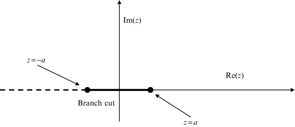
An important extension of this occurs when we evaluate (z²−a²)^1/2, where a is real, because if it is evaluated directly as [z²−a²]^1/2 then the result will only have a positive real part. In some applications that is a requirement, but in others, such as in potential flow, we need to evaluate this function for all values. To eliminate the ambiguity we specify the function as

${\left(z^2-a^2\right)}^{1/2}={\left[z-a\right]}^{1/2}{\left[z+a\right]}^{1/2}$

This function has two branch points, as shown in Fig. B.2, and the branch cuts from each branch point extend to −∞ on the real axis. However, when z<a on the branch cut both [z−a]^1/2 and [z+a]^1/2 have a phase shift of π and so the net phase shift is 2π, and the function is continuous. The remaining part of the branch cut forms a slit in the complex plane between z=−a and z=a.

We can extend this concept and define branch cuts at different angles for each point, and allow the branch points to be at some arbitrary location z_o so

${\left(z^2-z_o^2\right)}^{1/2}={\left[\left(z-z_o\right)e^{-i\left({\vartheta }_1+\pi \right)}\right]}^{1/2}{\left[\left(z+z_o\right)e^{-i\left({\vartheta }_2+\pi \right)}\right]}^{1/2}{e}^{i\left({\vartheta }_1+{\vartheta }_2\right)/2+i\pi }={\mathrm{R}\mathrm{e}}^{i\varphi }$

where the phase lies in the range

$\frac{{\vartheta }_1+{\vartheta }_2}{2}<\varphi <\frac{{\vartheta }_1+{\vartheta }_2}{2}+2\pi$

An example is shown in Fig. B.3 in which the branch cuts have angles ${\vartheta }_1=0$ and ${\vartheta }_2=-\pi$. We can also specify the phase ϕ using the angles to the branch cut defined in Fig. B.1B. These give

$\varphi =\left({\phi }_1+{\phi }_2\right)/2+\left({\vartheta }_1+{\vartheta }_2\right)/2$

For example, in Fig. B.3 we see that on the imaginary axis at z=i∞ the value of (φ₁+φ₂) is 2π, but in the vicinity of the origin it is reduced to a minimum but is never less than π. At z=−i∞ the value has increased again to 2π. On the imaginary axis it follows that the phase ϕ must lie in the range

$0<\varphi <\pi /2$

and so this choice of branch cut ensures that the function ${\left(z^2-z_o^2\right)}^{1/2}$ has a positive real and imaginary part on the imaginary axis.