
The equations of fluid motion
Abstract
This chapter is a review of the basic equations and concepts of fluid dynamics. These also form the foundations of aeroacoustics. We will start by considering the equations of fluid motion, the thermodynamics of small perturbations, and the role of vorticity. We will then evaluate the propagation of energy in the fluid, including the energy associated with sound waves in a moving medium, sound power, and acoustic intensity. Finally, we will review some basic concepts of fluid dynamics and summarize some results and methods of ideal flow theory that are most relevant to low Mach number aeroacoustics.
Keywords
Equations of fluid motion; Momentum; Continuity; Speed of sound; Energy equation; Sound power; Ideal flow; Conformal mapping
This chapter is a review of the basic equations and concepts of fluid dynamics. These also form the foundations of aeroacoustics. We will start by considering the equations of fluid motion, the thermodynamics of small perturbations, and the role of vorticity. We will then evaluate the rate of change of energy in the fluid, including the energy associated with sound waves in a moving medium. Finally, we will review some basic concepts of fluid dynamics and summarize some results and methods of ideal flow theory that are most relevant to low Mach number aeroacoustics.
2.1 Tensor notation
Cartesian tensor notation is useful in aeroacoustics because it provides relatively simple expressions for tensor products. In this section we will give a brief overview of the notation to be used in the following sections.
We are typically concerned with position vectors such as x and y which describe the locations of observers and sources, and flow variables, such as the velocity vector v, which defines the velocity of a fluid particle at a fixed location. In Cartesian coordinates these vectors have three components and if we use tensor notation, each component of the vector is defined by a subscript, say i, which has the values 1, 2, or 3. Hence we define x=(x1, x2, x3) giving the three components of the position vector x. To simplify the notation, we replace x by xi where the subscript i=1, 2, 3 defines each component. Using this approach, the definition of a dot product between the vectors q and v is

In general, the summation signs in the above definition are found to be cumbersome and so we introduce the convention that whenever repeated indices occur in a product there is an implied summation over all the components. Hence we have

For example, we can define the magnitude squared of a vector as

This notation is particularly useful in the definition of the gradient of a scalar ϕ

where i, j, and k are unit vectors in the i=1, 2, and 3 directions. Similarly, the divergence of a velocity v is

This approach is most valuable when dealing with tensors. For example, the product Sij=vivj is a tensor which represents a matrix with nine elements corresponding to i=1, 2, 3 and j=1, 2, 3.

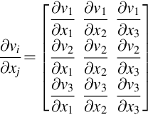
A common expression found in the equations of motion is the velocity gradient tensor ∂vi/∂xj, which expands as
Care needs to be exercised when we consider the expression Sii since this has repeated indices and so, by the rules defined above

Hence if we want to isolate only one of the diagonal terms of the tensor we write Sii (no summation implied).
Example
Consider the tensor defined by the Kronecker delta function δij (which is defined as zero when i≠j and one when i=j) and evaluate (a) pδij, (b) δkjδik, and (c) Sijδij.
Using the summation rule we obtain

Throughout this text the velocity vector is denoted as v or vi and is often considered as the sum of the mean, time invariant, velocity U and the velocity fluctuation about the mean u, so v=U+u. Coordinates are defined using the vectors x, y, or z with the coordinates x and y used to denote observer and source location, respectively, where relevant. A volume is denoted as V and a surface area by S.
The thermodynamic variables of pressure, density, temperature are given their usual symbols p, ρ, Te, and the internal energy, enthalpy, and entropy are expressed, per unit mass, using the variables e, h, and s, respectively. Stagnation enthalpy and specific total energy are H and eT, respectively. A subscript “o” is used to denote the mean, time invariant, values of the thermodynamic variables at a fixed location, whereas a prime is used to indicate the fluctuating part. The mean speed of sound is given by the symbol co, and if this is constant throughout the fluid the symbol c∞ is used.
2.2 The equation of continuity
The concept of conservation of mass requires that mass is neither created nor destroyed in any fluid element. In Fig. 2.1 we show a region of the fluid, which is of volume V, and is bounded by the surface S. We will refer to this as a control volume. The outward pointing normal to the surface is n(o) and the velocity of the fluid is v. If the volume is fixed in space, and the density of the fluid is written as a function of space and time t as ρ(x,t), then the mass of the fluid contained in V is


The flow transports fluid in and out of the control volume and the mass flux out of V, across the surface element dS, per unit time, is given by
The rate at which the control volume loses mass must equal the net outward flux of mass, which is given by the integral of Eq. (2.2.2) over the bounding surface S. Hence, for a fixed stationary surface

We can simplify this equation by using the divergence theorem to turn the surface integral into a volume integral. The divergence theorem states that the integral of the divergence of a vector over a volume is related to the component of the vector normal to the surface enclosing the volume by

Using this relationship gives

This result is independent of the volume V and so the integral can only be identically zero if the integrand is zero. Hence we obtain the continuity equation in differential form as

In tensor notation this is given as

This is one of the most important equations in fluid dynamics and defines how mass is conserved in a fixed volume. It shows that the rate of change of density with time added to the divergence of the mass flux is zero at a fixed point.
It is also important to consider how mass is conserved in a frame of reference that moves with a differentially small piece of the fluid material, defined as a fluid particle. To consider this, we introduce the substantial or material derivative Df/Dt, which defines the rate of change of the function f in a frame of reference that moves with the particles rather than in the fixed frame which was used above. To define the moving frame of reference, we specify the position of the fluid particles at time t1 by the vector ηi. Since the particles move with velocity vi their location at the time t>t1 will be

The rate of change in the convected frame of reference is the rate of change of f(zi(t),t) when ηi is fixed. Hence
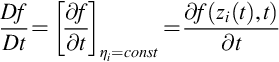
Then by using Eq. (2.2.7) and evaluating the partial derivatives we find the substantial derivative for the location xi=zi(t) in fixed coordinates is

The substantial derivative can now be used to rewrite the continuity equation: by using the vector identity ![]() , we expand Eq. (2.2.5) as,
, we expand Eq. (2.2.5) as,

This shows that if the fluid density is constant in the frame of reference moving with the fluid particles, so Dρ/Dt=0, then the divergence of the flow velocity is zero. In an incompressible fluid such as water, the density is almost constant and so we can approximate the requirement for conservation of mass as ![]() . However acoustic waves are, by definition, compressible and so this approximation cannot be used in the analysis of sound.
. However acoustic waves are, by definition, compressible and so this approximation cannot be used in the analysis of sound.
In the following sections we will consider thermodynamic quantities such as entropy or enthalpy, which are defined per unit mass rather than per unit volume. We will therefore need to consider the volume per unit mass, or specific volume, equivalent to the inverse of the density. We then have

and so Eq. (2.2.10) gives

This is an alternative form of the continuity equation, which is useful in applications that involve compressible flow.
2.3 The momentum equation
2.3.1 General considerations
To determine the momentum balance in a fluid we recall that the time rate of change of momentum of a body of fluid is equal to the net force exerted on it. We now apply this principle to the control volume illustrated in Fig. 2.1. The net momentum of the fluid in the control volume is given by

According to the conservation of momentum, the rate of change of this quantity equals the force F applied to the control volume less the net rate at which momentum leaves the volume due to the movement of fluid across its surface. We saw above that the mass flow rate of fluid across a single element of the control surface dS is ![]() . The rate at which momentum is lost due to this motion is therefore
. The rate at which momentum is lost due to this motion is therefore
Hence the rate of change of momentum in the fixed stationary control volume is

The forces which are applied to the control volume are of three different types: (i) body forces, such as gravity which are almost never important in aeroacoustic applications and so will be ignored, (ii) pressure forces which apply a net force −pn(o)dS to each surface element shown in Fig. 2.1, and (iii) viscous shear stresses that introduce a net shear force on the surface. Viscous forces are rarely important in sound waves but are often important to the flows that produce them. They are most conveniently expressed using a viscous stress tensor σij which gives the force per unit area in the j direction applied to a surface whose outward normal lies in the i direction. The stress tensor is symmetric so σij=σji and the indices are interchanged without consequence. We can define the viscous shear stress applied to the surface of the control volume as
where nj(o) is the tensor notation for the outward pointing normal to the surface. It is convenient to combine the viscous stress and pressure force into a single tensor pij defined as
This tensor is called the compressive stress tensor and is often used in aeroacoustics to replace the tensor τij=−pij which is more commonly used in texts on fluid dynamics.
These conventions allow the force on the fluid F in the control volume to be written as

Combining this with Eq. (2.3.3) yields, in tensor notation,

and applying the divergence theorem then gives

As with the continuity equation this integral can only be zero if the integrand is zero so we obtain the momentum equation in the absence of body forces as

This is the conservation form of the momentum equation, which shows that the rate of change of momentum of a fixed volume of fluid is balanced by the flux of momentum out of the volume and the stresses applied to its surface.
We can also write the momentum equation in a nonconservation form which relates the forces applied to a fluid particle to its acceleration Dvi/Dt. Newton's Second Law of motion then requires that the mass per unit volume ρ times the acceleration equals the force applied to the particle per unit volume, which from Eq. (2.3.6) and the divergence theorem is −∂pij/∂xj, so

It is a relatively simple exercise to show that Eqs. (2.3.9), (2.3.10) are the same by expanding the derivatives in Eq. (2.3.10) and using the continuity equation (2.2.6). Eq. (2.3.10) is the well-known Navier Stokes equation.
2.3.2 Viscous stresses
Viscous stresses are caused by molecular diffusion across the boundary enclosing the control volume. If the molecular diffusion causes fluid molecules to move into a region of fluid with a different velocity, then momentum is transferred and a viscous stress exists. The viscous stress causes the velocity parallel to the boundary, say vs, to be sheared in the direction normal to the boundary, so nj(∂vs/∂xj)≠0 or the velocity normal to the boundary, say vn, to be sheared in the direction parallel to the boundary, so (∂vn/∂xj)≠0. Detailed consideration of the viscous shear stress for a compressible fluid is discussed in texts on fluid dynamics [1,2], and requires the definition of a coefficient of bulk viscosity in addition to the shear viscosity μ. The bulk viscosity is usually assumed to be zero (Stokes hypothesis) in which case the viscous stress term is

where μ is the coefficient of viscosity (for a detailed derivation of this equation see Batchelor [1] or Kundu [2]).
The viscous stress term in the momentum equation can be simplified for an incompressible flow. From Eq. (2.3.10) we note that the contribution of the viscous stresses will depend on ∂σij/∂xj and that for an incompressible flow ∂vj/∂xj=0 so we obtain from Eq. (2.3.11)
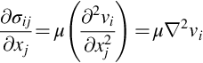
assuming constant viscosity.
The importance of the viscous term can be assessed by writing the Navier Stokes equations in terms of dimensionless variables. We define the dimensionless velocity, distance, time, density, and pressure ![]() ,
, ![]() , t#=Ut/L, ρ#=ρ/ρ∞, and p#=p/ρ∞U2 where U, L, and ρ∞ are constant reference values with L representing the overall scale of the flow. Substituting these definitions into Eq. (2.3.10), expanded using Eqs. (2.3.5), (2.3.11), gives
, t#=Ut/L, ρ#=ρ/ρ∞, and p#=p/ρ∞U2 where U, L, and ρ∞ are constant reference values with L representing the overall scale of the flow. Substituting these definitions into Eq. (2.3.10), expanded using Eqs. (2.3.5), (2.3.11), gives

Dividing throughout by ρ∞U2/L we obtain

We see that in normalized form the viscous term is divided by the ratio of the scale of the inertial forces ρ∞U2/L to the scale of the viscous forces μU/L2. This ratio is defined as the Reynolds number Re. In high speed and/or large scale flows the Reynolds number is high and the viscous term small, indicating that the effects of viscosity can often be ignored.
2.4 Thermodynamic quantities
Acoustic waves are a result of compressible effects in the fluid that cause small perturbations in the local pressure. It is therefore important that we understand how pressure changes are associated with changes in density and temperature. We make the assumption that an acoustic wave is a thermodynamic process which does not involve any exchange of heat or dissipative processes. In this case, the pressure perturbation p′ about the mean pressure po is directly proportional to the density perturbation ρ′ about the mean density ρo with the constant of proportionality given by the isentropic bulk modulus (dp/dρ)s.

We will show later that co is the speed at which sound waves propagate through the medium.
We cannot ignore the role of dissipative processes or heating on the generation of sound or on the flows that generate it. For this reason, we need to discuss the thermodynamic properties of gases in some detail and define the role of quantities such as the enthalpy and entropy, which along with pressure, density, internal energy, kinetic energy, and temperature, define the “state” of the gas.
The First Law of Thermodynamics requires that the energy of a system can only be changed by the addition of heat or by work done on the system. In this case our “system” is a fluid particle that (by definition) moves with the flow and has constant mass. The change of internal energy per unit mass of the particle de is given by the sum of the heat added per unit mass δq and the work done on the system per unit mass, δw, so
Note here that the internal energy represents the state of the particle and is independent of how the energy got there, whereas the heat and the work represent path functions and are dependent on the process taking place.
First consider what happens when the molecules in a particle expand to fill a larger volume. When the particle expands from a volume V to a volume V+dV, the work done on the surrounding fluid is given by the force exerted on the surrounding medium times the distance it moves during the expansion. Writing this as a surface integral, the force on each surface element is pdS, and the distance it moves is Δx, giving the total work done by the particle as

where the surface S encloses the volume V. Since the particle is very small the pressure may be considered as constant over the surface and, since

the work done by the system on its surroundings is pdV. This represents a loss of energy to the system and so Eq. (2.4.2) becomes
In this equation dυ represents a change in volume per unit mass and can be related to the density of the fluid in the particle using υ=1/ρ. This example considers a volumetric change which occurs at constant pressure. In many cases we need to consider changes in pressure which occur without a change in volume. In this case the particle increases its “capacity to do work.” We can define this capacity using a state variable called the enthalpy which is related to the internal energy as h=e+pυ. We note that dh=de+υdp+pdυ which allows the first law (2.4.3) to be written for a change at constant volume as

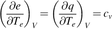
If heating takes place at either constant volume or constant pressure, then the temperature Te of the system is increased. The sensitivity coefficients are defined as specific heats for constant volume and constant pressure as

Hence if heating takes place at constant volume then the change in internal energy can be related to the heat input by Eq. (2.4.3). Specifically,
In contrast if heating takes place at constant pressure then we can use Eq. (2.4.4) to give the change in enthalpy as,

If e and h are only functions of temperature (the assumption of a perfect gas), then these expressions reduce to de=cvdTe and dh=cpdTe. Subtracting Eq. (2.4.3) from Eq. (2.4.4) and using these relationships give
or
which integrates to the perfect gas law p=ρRTe with R=(cp−cv).
For an ideal gas the specific heats are constant and allow us to relate the internal energy and the enthalpy to the temperature as
To proceed further we introduce the concept of the entropy of a system, which describes its state of disorder. Entropy is a variable like temperature or pressure that gives the state of a gas. It is increased by the addition of heat and by any irreversible process, like heat conduction or molecular diffusion. The Second Law of Thermodynamics gives the entropy change in a process as

where δqrev is called the reversible heat addition. This is an imaginary quantity—heat cannot be added reversibly as the addition will always be accompanied by some dissipative process that would further increase disorder. So δqrev is the amount of heat that would have to be added, in the absence of any accompanying dissipative process, to account for the thermodynamic changes that occur due to irreversible processes and any actual addition of heat. We can use Eq. (2.4.7) and the first law to obtain a relationship for entropy in terms of the other state variables. Imagine a process containing only reversible heat addition. In this case we would have δq=δqrev and we could substitute Teds in Eq. (2.4.7) for δq in Eqs. (2.4.3), (2.4.4). This would give

Notice that these expressions give the entropy change only in terms of the other state variables p, ρ, Te, e, and h. We can therefore infer that Eq. (2.4.8) must hold in general (not just for our reversible example), unless entropy defines a property of the gas independent of these other variables. This is not the case. For example, for a thermally perfect gas the Kinetic Theory of Gases tells us that any of the state variables can be expressed as functions of two others.
So, by rearranging these equations using Eq. (2.4.6),

then using the perfect gas law, we find

from which it follows that the specific entropy is
where C is the constant of integration and γ=cp/cv is the ratio of specific heats. We see then that for s=const we have

Differentiating this equation, we obtain the isentropic bulk modulus,

This expression is of course, equal to the sound speed squared (Eq. 2.4.1). However, for sound waves the pressure fluctuations p′ and density fluctuations ρ′ are very much less than their mean absolute values, so in this case we can replace the pressure and density with their mean values po and ρo to give

We can also reinterpret Eq. (2.4.9) as an expression for the small changes in a sound wave. For fluid flows where the entropy is the same everywhere (i.e., only isentropic processes occur, and the entropy at all points has the same initial value) the flow is defined as homentropic, so ds=0, and

giving ![]() , which is the expression given by Eq. (2.4.1).
, which is the expression given by Eq. (2.4.1).
A more general specification is isentropic flow, in which the specific entropy of each moving particle is constant so Ds/Dt=0. This leads to a generalized relationship between pressure and density which is obtained by taking the substantial derivative of Eq. (2.4.8), and using Eq. (2.4.6), to obtain

We solve these equations to obtain a relationship between pressure and density fluctuations for an isentropic flow as

where γp/ρ is the local instantaneous sound speed squared, or,

if the flow generated fluctuating pressure and density are small compared to their absolute values, as is usually the case in low Mach number flows. Comparing these results with Eq. (2.4.11) shows that for an isentropic flow the relationship between pressure and density depends on their material derivatives, as distinct from their perturbations from the mean, but the constant of proportionality is the same when the mean pressure and density are used. In the following section we will consider the entropy of the fluid in more detail and show when we can make the assumptions of homentropic and isentropic flow.
2.5 The role of vorticity
2.5.1 Crocco's equation
Irrotational flows are important in fluid dynamics and to put their features in perspective we need to consider the role of vorticity. We start by rearranging the momentum equation into a form which was originally derived by Crocco. This relates the rate of change of velocity to terms such as the vorticity. To obtain Crocco's equation we expand the momentum Eq. (2.3.10) term by term and divide by ρ so

where e is a vector specifying the viscous force per unit mass defined in tensor notation as ei=(1/ρ)∂σij/∂xj and the kinematic viscosity ν=μ/ρ. We can rearrange this expression by making use of the vector identity
with u=v to obtain
and so

where we have introduced the vorticity, defined as ω=∇×v. The term ![]() is replaced by introducing the stagnation enthalpy, defined as
is replaced by introducing the stagnation enthalpy, defined as ![]() . We then rewrite Eq. (2.4.8) in terms of gradients as
. We then rewrite Eq. (2.4.8) in terms of gradients as

This assumes that at some upstream point the fluid properties are initially uniform in space, so that their values at adjacent points can be thought of as being connected by a single thermodynamic process. Substituting from the definition of the stagnation enthalpy we obtain,

This is substituted into Eq. (2.5.3) to give

This is Crocco's form of the momentum equation, which highlights some of the most important features of inviscid, irrotational flow.
If the flow is irrotational (∇×v=ω=0), then the velocity can be expressed as the gradient of a scalar field, v=∇ϕ since, by definition the curl of the gradient of any scalar field is zero. We refer to ϕ as the velocity potential. If the flow is also homentropic (∇s=0) and inviscid (e=0) Eq. (2.5.4) reduces to ∇(∂ϕ/∂t+H)=0, from which Bernoulli's equation is obtained by integration to give

where f(t) is constant across all space. This is important because it shows that for an irrotational, inviscid, and steady flow, H=const≡Ho throughout the flow. This is the basis for potential flow calculations in fluid dynamics, which provide great insight into simple flows around streamlined bodies. If the flow is unsteady, but the unsteadiness occurs over a limited region of space embedded in an ambient steady flow, then Eq. (2.5.5) applies but f(t) must be a constant equal to the ambient stagnation enthalpy. Thus we write

where H′ is the unsteady stagnation enthalpy.
2.5.2 The vorticity equation
We can now derive an equation for the vorticity from the curl of Eq. (2.5.4) as

This may be written in nonconservative form by using the vector identity
We note that, since the divergence of any curl field is zero, ∇·ω=0. We can then make use of Eq. (2.2.12) to rewrite Eq. (2.5.6) as

We then use Eq. (2.3.11) and the definition ei=(1/ρ)∂σij/∂xj to evaluate ∇×e. Since the curl of a gradient is zero we obtain ∇×e=ν∇2ω, assuming constant viscosity. Finally, dividing by ρ and combining terms give the compressible vorticity equation

This equation defines the generation and modification of vorticity in any fluid. When viscous and heating effects are absent the evolution of vorticity within the flow is determined by the second term in the equation which represents the distortion of the fluid particle by the velocity gradients. In two-dimensional flow the vorticity vector is normal to the direction of the flow gradient and so this term is zero. We also note that Eq. (2.5.8) is a set of nonlinear homogeneous differential equations for the vorticity vector, whose terms describe the transport, deformation, generation, and diffusion of vorticity. We will discuss the fluid dynamics of vorticity and its implications, in more detail in Section 2.7.
2.5.3 The speed of sound in ideal flow
Before concluding this section, it is worthwhile considering the definition of the speed of sound in a little more detail and showing how it depends on the local flow conditions for an ideal gas in steady flow. We have shown that for a homentropic (inviscid), steady, irrotational flow originating in a uniform free stream, the stagnation enthalpy is constant. If we define upstream or reference conditions using the subscript ∞ then we use Eq. (2.4.10) and Ho=const to give
where U is the mean flow speed and the subscript o represents mean quantities at the downstream location, while the subscript ∞ refers to upstream conditions. To obtain the speed of sound we note that h=e+p/ρ and that Eq. (2.4.6) allows us to write h=γe. Combining these relationships gives h=γp/ρ(γ−1), and using Eq. (2.4.11) we obtain from the second part of Eq. (2.5.9)

where co is the local speed of sound and c∞ is the speed of sound at the upstream location. Furthermore, using the first equation of Eq. (2.5.9) gives relationships for the local mean pressure and density as

Hence given a set of upstream conditions and a homentropic mean flow, we can determine the variation of speed of sound, mean density, and mean pressure from the local flow velocity alone. We conclude that the speed of sound and the density can be taken as constant in applications where ![]() , which is usually the case in low Mach number flows.
, which is usually the case in low Mach number flows.
2.6 Energy and acoustic intensity
2.6.1 The energy equation
The equations of state which define the speed of sound propagation have been shown to be dependent on the distribution of the mean thermodynamic properties of the gas and can be simplified if it can be assumed that the flow is either homentropic or isentropic. We therefore need to define an equation that determines the conditions that allow these assumptions to be made. This is achieved by considering the rate of change of energy of a fluid particle as it moves through space. The total energy per unit mass of the particle eT is given by the sum of its specific internal energy e and its kinetic energy per unit mass ![]() . The rate of change of energy for the fluid particle is then
. The rate of change of energy for the fluid particle is then

where M is the mass of the particle, and the material derivative is required because we are considering a constant mass of fluid which is moving through the medium. From the First Law of Thermodynamics the energy of the particle only changes if the particle does work on the surrounding fluid or it is the recipient of heat. If the particle occupies a small volume V(t) at time t then the rate of work done by the particle is determined by the stresses on the surface S(t) enclosing the particle, and the velocity of the surface. The rate of work done on the particle by the surrounding fluid is the negative of this,

where ni(o) is the outward pointing unit normal to the surface. If heat flux per unit area through the fluid material is given by the vector field Q, then the flow rate of heat energy into the particle is,

Using the divergence theorem, we can change the surface integrals in the above two equations into volume integrals and write the rate of gain of energy of the particle as

We can then equate (2.6.2) to the net increase in energy given by Eq. (2.6.1), as

Since the particle is very small we can assume the integrand is constant throughout the volume and define the density as ρ=M/V(t) to obtain the energy equation

This equation relates the rate of change in total energy of a fluid particle to the rate of work done by surface stresses and the rate of heat addition. We have neglected body forces such as gravity in this derivation since these effects are rarely important in acoustics.
We can also derive the rate of change of energy directly from the relationships given in Section 2.4. First we rewrite Eq. (2.4.8) in terms of substantial derivatives,

This is permissible because the rates of change in the thermodynamic variables experienced by a specific fluid particle over time constitute a thermodynamic process, regardless of the particle motion, and viscous action that may cause heating is considered negligible. Incorporating the specific total energy and multiplying by density gives,

The second term on the right of this equation can be simplified using Eq. (2.2.12) and the third term may be reduced using the momentum equation (2.3.10) so

This gives the energy equation in terms of the entropy rather than the heat flux vector, which may be useful in some applications. An important result is obtained if we subtract Eq. (2.6.6) from Eq. (2.6.4) to give

This shows that if we can ignore viscous effects and heat conduction then the flow can be considered as isentropic, and relationships such as Eq. (2.4.14) can be used to relate the pressure and density fluctuations in the fluid. This is an important result because direct viscous effects are negligible over large parts of most engineering flows. Similarly, in acoustic waves the momentum flux is almost completely balanced by pressure perturbations and viscous effects on acoustic propagation are found to be very small. Further, in most fluids flows the temperature is uniform or varies only slowly on the scale of wave propagation, so heat conduction effects are not significant. Hence the assumptions required of an isentropic flow apply to most of our applications. Entropy fluctuations are caused by a burst of heat such as a combustion event in the flow, and entropy is a convected quantity in the absence of viscous effects or heat generation. Therefore, if s=0 at an upstream location in an inviscid unheated flow, then it remains zero throughout the flow.
In Eq. (2.6.4) the energy equation is given for a material element, which is convected through the fluid. We can also express this for a stationary point in space by using the continuity equation to provide the expansion

Writing in tensor notation we have,

Using Eqs. (2.6.8), (2.6.4) then gives,

Further simplification is possible by introducing the stagnation enthalpy which is equal to H=eT+p/ρ, so

This result gives the rate of change of total energy at a point in terms of the flux of enthalpy, the viscous stresses, and the flux of heat. It is valuable because it can be integrated over a fixed control volume of any size, to give the rate of change of total energy of a system. For example, if we consider a jet engine and draw a control volume as a spherical surface of very large diameter enclosing the engine and its exhaust, the volume integral of ∂(ρeT)/∂t inside the control volume gives the net rate that energy is added to the fluid. If energy is being lost from the control volume, then it must be replaced at the same rate by the engine to maintain a steady outflow. The rate at which energy leaves the control volume is equal to the instantaneous power being generated by the engine WT. If the control surface is far enough from the engine, so that viscous effects and heat conduction are zero on the control surface, then Eq. (2.6.10) shows that the total power generated by the engine can be obtained from

This result is valuable in the experimental evaluation of engineering systems because it allows for the mechanical input of power to the fluid to be determined directly from measurements on a surface surrounding the power source. It is also useful in acoustics because it leads to the concept of sound power generation, and allows us to define acoustic source strength from measurements at great distances from the source of sound.
2.6.2 Sound power
As noted above the power generated by a system is an instantaneous quantity, which means that WT will vary with time. Furthermore Eq. (2.6.11) includes power needed to drive the system as well as the power required to maintain the unsteady flow and the acoustic waves, which may be a small fraction of the total. In acoustic applications we are interested in making this distinction and separating the mechanical power generated by the system from the “power” required to feed the acoustic motion of the fluid particles at large distances from the source. To make this distinction let us consider the average power generated by the system over a period of time. We will define this as the “expected value” of the instantaneous power and split it into contributions from the steady Ws and unsteady part (time varying) Wa, so
where E[] represents an expected value. The steady components of the flow quantities are defined using the subscript o and unsteady parts with primes so H=Ho+H′ etc. The mass flux per unit area is then ρv=E[ρv]+(ρv)′. The unsteady components will have a zero mean value, but their correlations can be nonzero. Hence terms like E[(ρv)′Ho] are zero, but terms like E[(ρv)′H′] are nonzero and contribute to the unsteady power budget. As discussed above we choose to split the power budget as
and
The reason for this choice is that in a homentropic potential flow we can show that Ws is zero because, according to Crocco's equation, Ho is constant over space and Eq. (2.6.13) reduces to

using the continuity equation. We conclude that a steady inviscid potential flow does not need to be driven by a power source. In contrast we would expect a real flow, which includes turbulent wakes and viscous effects, to require a source of power to maintain it in a steady state, so Ws≠0. On this basis we define Ws as the mean power and Wa as the power from unsteady enthalpy, which we will later relate to acoustic processes. The splitting of power in this way allows us to define a procedure for measuring the sound power output Wa of an acoustic system. In general, we define
where I is the acoustic intensity in the region outside of the turbulent flow. Then, if we can measure the acoustic intensity on a surface enclosing the sources of sound, we can determine their sound power output. This has proven to be a useful concept in noise control applications provided we can accurately determine I. For a homentropic flow we use Eq. (2.4.8) to give H′=p′/ρo+U·u (note that to first order accuracy ![]() so the unsteady part of
so the unsteady part of ![]() is Uiui) so
is Uiui) so
We conclude that in order to measure the acoustic intensity in a flow, we need to know the flow speed as well as the acoustic perturbations of density, particle velocity, and pressure. The measurement is much easier in a stationary medium for which I=E[p′u] and instrumentation is commercially available to measure this quantity directly. However, some care needs to be exercised because Eq. (2.6.17) is not uniquely related to the acoustic processes in turbulent flow where unsteady pressure and velocity fluctuations can exist that do not propagate as acoustic waves.
2.7 Some relevant fluid dynamic concepts and methods
In addition to the governing equations, an appreciation of some of the physics of fluid dynamics and the methods used in its analysis is needed as a basis for aeroacoustics. The purpose of this section is to provide a short review of this topic. Readers who need or desire a more in-depth treatment are referred to dedicated texts in this field such as Karamcheti [3], Howe [4], or Katz and Plotkin [5].
2.7.1 Streamlines and vorticity
One of the most commonly used concepts of fluid dynamics is that of a streamline. A streamline is simply a line that is everywhere tangent to the velocity vector. It follows that the streamlines are given by the equation ds×v=0 where ds is change in position along the streamlines. The concept of a streamline is particularly useful in steady flow, since in this case the streamlines are also the paths taken by fluid particles. In unsteady flows where the velocity fluctuations are small compared to the mean, the streamlines of the mean flow can still be taken to represent the overall paths taken by the fluid, as well as the paths along which turbulence is convected.
Consider a curve in space that cuts across a flow as shown in Fig. 2.2. All the streamlines that pass through this curve will form a stream surface. By definition there can be no flow through a stream surface as it is everywhere tangent to the flow. Mathematically we can define a family of stream surfaces by representing them as contour surfaces of a scalar function ψ, known as the stream function. Charting all the streamlines that pass through a pair of intersecting curves (Fig. 2.2) maps out two intersecting stream surfaces of different families. The intersection of these surfaces must be a streamline and aligned with v, and the perpendiculars of these surfaces (aligned with the gradient of their respective stream functions) must both be perpendicular to v. We therefore have that

where α is some scaling factor. Since the divergence of the cross product of two gradient fields is identically zero, we must have that ∇·(αv)=0. In steady flow we can choose α to be the flow density since then this condition is satisfied by virtue of conservation of mass, Eq. (2.2.6). When the flow is incompressible α can equally well be taken as 1. Stream functions and streamlines are key quantitative concepts particularly with reference to rapid distortion theory and the drift function, topics to be covered in Chapter 6.
We can analogously define vortex lines, lines everywhere tangent to the vorticity vector that can be thought of as instantaneously stringing together the axes of rotation of adjacent fluid particles (the vorticity is twice the angular velocity of the fluid particles). Being a rotational field, the divergence of the vorticity is identically zero and thus from the divergence theorem we have that the net flux of vorticity out of any closed surface is zero

because the divergence of a curl operation is zero. This is valid regardless of the flow, the fluid, or the thermodynamic conditions and can be interpreted as saying that all vortex lines entering a volume must exit from it and thus, all vortex lines must continue to infinity or form loops. This is one of Helmholtz' vortex theorems.
Rotation in a fluid on a macroscopic scale is measured in terms of circulation Γ, the integral around a closed loop C of the velocity component along the loop:

Circulation and vorticity are related through Stokes' theorem, which states that the circulation around a loop is equal to the net flux of vorticity through any open surface bounded by that loop:

where n(o) is a unit normal vector pointing out of the surface, this direction being given by the right-hand rule applied to the direction of the line integral around loop C. This too is a mathematical identity, but one containing subtleties. For example, Eq. (2.7.4) cannot be applied to just any loop because not all loops bound surfaces over which the vorticity is defined. A case in point is steady irrotational flow around a two-dimensional airfoil of infinite span. For any loop that contains the airfoil, no surface can be drawn bounded by that loop that does not pass inside the airfoil where the vorticity is undefined. Thus Stokes' theorem cannot be applied and we can have a circulation around the airfoil even though the flow has no vorticity. In the real flow about an airfoil the vorticity is trapped in the airfoil boundary layer and wake as we will demonstrate below. Note that in the irrotational flow, all loops that pass around the airfoil have the same circulation since two loops of different sizes form the perimeter of an annular surface on which we can apply Stokes' theorem.
The rate of change of circulation around a loop of fluid particles that convects with the flow is DΓ/Dt, which can be written, starting with Eq. (2.7.3), as:

Since ds represents the distance between adjacent fluid particles in the fluid loop, the rate of change of this seen moving with the flow D(ds)/Dt is merely the difference in velocity between the particles dv. Since ![]() and vi2 will have the same value at the beginning and end of the loop, the last integral is zero. Substituting the momentum equation (2.5.1) for Dv/Dt we obtain,
and vi2 will have the same value at the beginning and end of the loop, the last integral is zero. Substituting the momentum equation (2.5.1) for Dv/Dt we obtain,

This is Kelvin's circulation theorem. The terms on the right-hand side are called the pressure force torque and viscous force torque, respectively. We can evaluate the pressure torque by applying Stokes' theorem to this line integral,

If the fluid is barotropic so that the density is a unique function of pressure (as in isentropic flow), or if the density is constant, then ∇ρ×∇p is always zero. In these situations, therefore, circulation can only be changed around a fluid loop as a consequence of viscous forces acting on that loop.
This has profound implications. Eq. (2.7.6) applies to a fluid loop, however small, including one wrapped around a single fluid particle. It therefore says that, in the absence of pressure and viscous force torques, the vorticity of a fluid particle will not change and if it is initially zero, then it will remain zero (this is the second of Helmholtz' theorems). Thus vorticity is convected with the flow as if it were part of the fluid material. In flows that begin with an irrotational free stream, vorticity will only appear where pressure or viscous force torques act.
A second implication is known as the starting vortex. Consider a stationary two-dimensional airfoil of infinite span in a stationary fluid. We define a fluid loop that encloses the airfoil (Fig. 2.3) and is large enough so as to remain outside any viscous flow generated once the airfoil starts moving. Obviously the circulation around this loop is zero and, according to Kelvin's theorem, will remain zero. The airfoil begins moving, developing a lift and therefore (as we will see below) a circulation. Vorticity is generated by viscous torques acting at the airfoil surface, and some of this is swept into the developing airfoil wake. For the circulation around the loop to remain zero, the circulation around this wake must be equal and opposite to that around the airfoil. We can apply a similar argument to any unsteadiness in the airfoil circulation once it is in motion and thus conclude that all such fluctuations must result in the shedding of vorticity of equal and opposite strength in the wake.

In incompressible flow the viscous force per unit mass can be calculated using Eq. (2.3.12) from the Laplacian of the velocity. Expanding this using vector identities gives,
where μ/ρ is the kinematic viscosity which is taken as a constant. We see that the viscous force is zero if the flow is irrotational. So, if a barotropic flow is initially irrotational then it will remain irrotational because it cannot produce viscous torques in the absence of a boundary, and without viscous torques no new vorticity can be generated. The implication is that vorticity and viscous effects can only originate at the flow boundaries and, in practice, this occurs at solid surfaces as a result of the no slip condition. To all intents and purposes, this is also true in compressible flows with low Mach number when the viscosity is constant, or nearly so, and where Eq. (2.3.12) is valid to an error of the order of the Mach number squared.
The no slip condition describes the observation that fluid immediately adjacent to a solid surface cannot move relative to it. This causes the formation of a boundary layer—a thin layer of fluid over the surface where the speed of flow is slowed by friction in the form of viscous forces. Boundary layers can be laminar but at high Reynolds numbers, or when disturbed, they become turbulent. Separated flows and wakes are always created from boundary layers. Vorticity generated by viscous action thus populates all these regions. When, as is usually the case, these flows are turbulent, much of the turbulence energy is contained in large organized eddies, also termed coherent structures or vortices. A classic example is the nearly regular train of eddies that can be shed into the wake of a bluff body, known as a vortex street. In most other flows, coherent structures are less organized than this, but are no less important in determining the dynamics of the flow and the sound it produces.
In aeroacoustics, turbulent motions are often referred to as gusts, commonly with the adjectives “turbulent” or “vortical.” The linearity of most aeroacoustics problems means that it makes sense to decompose these motions into sinusoidal components that are then considered separately, hence the mathematically useful but physically improbable concept of a sinusoidal gust. Given Helmholtz' vortex theorems, vorticity, coherent structures, and gusts are often conceptualized as being convected by the local time-averaged flow, implying, whether true or not, that these are small disturbances and that viscous force torques act on a timescale large compared to the others controlling the flow. This latter assumption requires that the ratio of the scale of the inertial forces to that of viscous forces is large, which implies high Reynolds number flow.
2.7.2 Ideal flow
In general, aerodynamic surfaces are designed to operate with low drag and thus with boundary layers that remain thin compared to the overall scale of the surface. Therefore, aerodynamic performance with the exception of drag can often be modeled by ignoring the boundary layer altogether and assuming irrotational flow. If the flow is of low Mach number, homentropic, and can be considered incompressible, then the governing equations become particularly simple and we refer to the resulting motion as ideal flow.
The governing equations of ideal flow are obtained by first considering the condition of irrotationality ∇×v=0, which is identically solved by expressing the velocity as the gradient of a scalar function ϕ, called the velocity potential (hence our previous references to potential flow in this chapter). Note that the absolute value of the velocity potential has no meaning since it is important only in that its gradient gives the velocity field.
Under the conditions of ideal flow, the momentum equation, in the form of Eq. (2.5.5), reduces to Bernoulli's equation for unsteady potential flow,

where the constant can be a function of time. The continuity equation (2.2.10) becomes simply ∇·v=0, or
This is, of course, Laplace's equation. The challenge of ideal flow is to find solutions to Laplace's equation that satisfy the boundary conditions of the problem at hand. Since, the continuity equation is only first order in terms of velocity we can only satisfy one boundary condition and thus we choose to satisfy the nonpenetration condition v·n=∂ϕ/∂n=0 on rigid surfaces, where n is a unit vector normal to the surface. The no slip condition is ignored since in any case our assumptions preclude modeling of the vortical boundary layer that it generates.
Many important aerodynamic results are obtained by considering the case of ideal flow in two dimensions. In this case we make use of the fact that any analytic function of a complex variable is a solution to Laplace's equation. As the independent variable we choose a complex coordinate z=x1+ix2 to define positions in the flow. As dependent variables we define the complex potential w(z) and complex velocity w′(z), where
The streamfunction ψ used to complete the complex potential is obtained from Eq. (2.7.1) with α=1, ψ=ψ1, and ψ2=x3, the latter representing the stream surfaces coincident with the x1-x2 planes in which the two-dimensional flow takes place. With these values we obtain v1=∂ψ/∂x2 and v2=−∂ψ/∂x1 (compared to v1=∂ϕ/∂x1 and v2=∂ϕ/∂x2). Note that the complex velocity is defined with its imaginary part equal to −v2 since in this case we have,

Since Laplace's equation is linear, the solution to complicated flow problems can be obtained through the superposition of simple solutions expressed as functions of the complex variable z=x1+ix2. To match the nonpenetration boundary condition of a solid surface the stream function, or the imaginary part of w(z), must be chosen to be a constant on that surface, and the solutions to many problems can be obtained by superimposing simple flows to meet this criterion. The complex velocity of some simple flows representing a point source, a vortex, and a doublet, are

where q, Γ, and A are real constants that denote the strength of these flows, z1 denotes their positions, and angle β denotes the orientation of the doublet. The free stream contribution to the flow is simply a constant w′(z)=U∞ exp(−iα) where α is the free stream angle. The flows of Eq. (2.7.12) all have singularities of infinite velocity at the point z=z1 where they are not analytic. Everywhere else, however, these are valid.
Fig. 2.4 illustrates the flows. The source is simply flow away from the point z=z1, the magnitude of the radial velocity decaying with the inverse of the radius. Despite appearances, this flow (as it must) satisfies conservation of mass everywhere except the singularity at its center, where fluid is produced at a volumetric flow rate of q per unit span. By convention a source with a negative strength is referred to as a sink. The vortex produces a flow that orbits the singularity with a tangential velocity that decays inversely with radius. This is an entirely irrotational flow outside the singularity, but one that has a circulation Γ around any loop that encloses the singularity. Consistency with Stokes' theorem is maintained in one of two ways. We can argue that Stokes' theorem doesn't apply since any surface bounded by a loop containing the singularity must pass through the singularity and therefore out of the domain where the velocity is defined. Alternatively, we can think of the point vortex as an idealization of an eddy where all the vorticity has been concentrated into a point at its center with a magnitude Γ. The vorticity is then given as Γδ(x1)δ(x2) and integration of the delta functions in Stokes' theorem yields the correct circulation. The doublet flow can be likened to a source and sink placed very close together. Flow is produced on one side of the doublet and is then reabsorbed on the opposite side. The orientation of the doublet, defined by the direction of flow along the single straight streamline that passes through its singularity, is set by the parameter β.

With equal validity we can think of the flow fields generated by adding these singularities as representations of steady flows or as snapshots of unsteady flows. For example, consider the flow generated by a point vortex of strength Γ placed at a height h above a plane solid surface, i.e., at z1=ih (Fig. 2.5). To satisfy the nonpenetration condition imposed at the surface the circular vortex flow must be modified. This modification is determined using the method of images, which says that the influence of the wall on a singularity is identical to the effect of adding the mirror image of that singularity in the wall. In this case, where the wall is coincident with the x1 axis, the image will be a counter-rotating vortex of strength −Γ at the location z1=−ih. Essentially the addition of the mirror image flow cancels out the wall-normal velocity component at the surface, making it a streamline of the flow. The complex velocity and complex potential of this flow, illustrated in Fig. 2.5B are thus,


where the complex potential is obtained by integration of the complex velocity according to Eq. (2.7.11). In these equations the second term represents the flow induced by the presence of the surface. This becomes an unsteady problem if we want the vortex singularity to represent the behavior and influence of a real flow feature, i.e., an eddy. The eddy will move as it is convected by the rest of the flow, and thus Fig. 2.5B represents only one instant of the flow history. To estimate the convection velocity in the ideal flow model we only need determine the velocity of the rest of the flow at the singularity, where “rest of the flow” includes the image representing the influence of the surface. The convection velocity wc′ is therefore determined by evaluating Eq. (2.7.14) at z=ih, ignoring the first term since that represents the vortex itself, to give ![]() . Noting that this is entirely real, we conclude that the vortex convects itself parallel to the surface. The ability of a point vortex to represent actual eddies in an idealized way makes it particularly useful in aeroacoustics.
. Noting that this is entirely real, we conclude that the vortex convects itself parallel to the surface. The ability of a point vortex to represent actual eddies in an idealized way makes it particularly useful in aeroacoustics.
As a second example, consider the steady flow past a circular cylinder. In its simplest form this can be simulated by placing an opposing doublet in a free stream, giving a complex velocity field of

It is left as an exercise for the reader to show that this flow, shown in Fig. 2.6A, contains a circular streamline centered at z1 of radius ![]() . Adding a point vortex at z1 does not change the circular streamline since the vortex velocity field is entirely tangential, but alters the flow to represent circulation around the cylinder (Fig. 2.6B). The complex velocity field, expressed in terms of the cylinder radius R is then
. Adding a point vortex at z1 does not change the circular streamline since the vortex velocity field is entirely tangential, but alters the flow to represent circulation around the cylinder (Fig. 2.6B). The complex velocity field, expressed in terms of the cylinder radius R is then


Of course, neither of the ideal flows shown in Fig. 2.5 are very useful as representations of the actual flow around a cylinder, which is dominated by the shedding of a thick rotational wake. However, as will be discussed below, the circular cylinder with circulation is useful as a starting point for airfoil analysis where ideal flow does provide realistic solutions. Note that in this example we have considered the singularities to be held in place at z1 and therefore representing a steady flow about a fixed cylinder.
A third example, with which we introduce the Milne Thompson circle theorem, combines the last two giving us the flow past a circular cylinder in the presence of a vortex. The Milne Thomson circle theorem enables us to introduce a circle of radius R centered at the origin, into any ideal flow w(z) as long as that flow contains no other rigid boundaries. With the circle, the complex potential becomes
where w⁎() is the complex conjugate of function w(), obtained by conjugating all the constants in w() (whether they are additive or multiplicative). This is easily proven by substituting the coordinates on the circle z=Rexp(iθ) where θ is angle measured from the real axis about the origin. We then obtain,
Thus the complex potential w1 is entirely real on the surface of the cylinder, implying that the streamfunction is constant, and thus the cylinder is a streamline. To proceed with our example, consider the flow generated by an isolated point vortex located at z1. From Eq. (2.7.12) we will have that

Applying the Milne Thompson theorem to add the cylinder to this flow we obtain

This flow field, shown in Fig. 2.7 can be understood by decomposing the second term in Eq. (2.7.20) which, by analogy with our plane wall example and Eq. (2.7.14), is referred to as the image of the vortex in the circle. Specifically, we can write


where the constant can be ignored since it has no impact on the velocity field. We see that the image consists of a point vortex at the cylinder center and another at R2/z1⁎ of equal and opposite strength to the original vortex, respectively. This vortex configuration is shown in Fig. 2.7 which shows that the position R2/z1⁎, referred to as the inverse point, lies inside the circle on the line joining the center of the circle to the position of the original vortex. Note the strength of image vortex at the center of the circle can be adjusted or set to zero so the net circulation around the cylinder is modified. This doesn't alter the circular streamline representing the cylinder since the vortex only generates tangential velocities.
As with the plane wall example, we can compute the convection velocity of the vortex by calculating the velocity produced by the rest of the flow at z1. This involves differentiating Eq. (2.7.21) and substituting z1 for z. Expressing the result in polar velocity components, which can be calculated as ![]() , we find that the vortex has no radial convection and moves tangentially with a velocity
, we find that the vortex has no radial convection and moves tangentially with a velocity

where r1=|z1|.
Returning to the uniform flow past a circular cylinder with circulation, Fig. 2.6B, it is clear that the flow passing through the cylinder is being deflected downward. To sustain this there must be an upward force on the cylinder, i.e., a lift. Lift is by definition a force perpendicular to the free stream. It is given by the Kutta Joukowski theorem which relates the lift force on any two-dimensional body in an otherwise undisturbed uniform flow to the circulation around it as,
which equals to −F2/b in terms of the span b and the force F2 acting on the fluid (the convention for forces in aeroacoustic analysis). Note that, the caveat “otherwise undisturbed” is important—any other disturbance to the flow around the body, say from a vortex, or a nearby surface or another body, invalidates this result. The Kutta Joukowski theorem can be derived from first principles or as a special case of the Blasius theorem. This gives the steady force per unit span integrated over any closed contour C (not just a body surface) in any ideal flow in terms of its components in the x1 and x2 directions as

Note that the sign of this expression has been chosen so that it gives the force on the fluid exterior to the contour rather than on the body or region inside. The force is therefore given by the residues of the function w′(z)2 at singularities within C. For example, Blasius theorem gives the force components on the vortex adjacent to the wall in Fig. 2.5 as F1=0 and F2=−ρΓ2b/4πh if use is made of the identity that

2.7.3 Conformal mapping
The complex representation of ideal flow permits flow solutions to be modified by conformal mapping. Specifically, any complex function z=z(ζ) can be used to map one coordinate pair, say, ζ=ξ1+iξ2 to another z=x1+ix2. This enables us to take a simple flow solution in terms of ζ, constructed using the methods described above, and transform it into a more sophisticated flow, in terms of z. Specifically, we can map a complex potential constructed in the ζ plane, W(ζ), to a new complex potential, w(z), in the z plane by writing
This transfers the value of the complex potential at the point ζ to the point z, and thus the streamlines of the flow are deformed in the same way that the mapping deforms the space. Since both w and W are functions of a complex variable, they are both solutions to Laplace's equation wherever these functions are analytic. We can get the complex velocity in the mapped domain w′(z) simply by differentiating

At points where the derivative of the mapping function dz/dζ=0, singularities can appear in the mapped flow that were not in the original flow. These are known as critical points. Everywhere else the mapping is referred to as conformal. Angles of intersection are preserved under conformal mapping, but not at critical points. Thus critical points are very useful for creating flow past a geometry with a sharp corner from one that is smooth (such as the circular cylinder). A good example and perhaps the most important example of mapping for aeroacoustics, is the Joukowski mapping. This is given by the function z=ζ+C2/ζ, where C is a real constant. This has critical points on the real axis at ζ=±C corresponding to z=±2C. The Joukowski mapping transforms the space outside a circle of radius C centered on ζ=0 in the ζ plane to the whole space by, effectively, flattening the circle on to a strip of length 4C on the real axis (Table 2.1). Angles of intersection are preserved everywhere except at the critical points at the end of the strip where they are doubled, for example from the 180-degree angle on the exterior of the circle to 360 degrees at the end points of the strip.
Table 2.1
Conformal mappings showing their effects on space
| Mapping function | ζ plane | z plane |
| Joukowski |  |  |
| Half-plane |  |  |
| Logarithm |  |  |
| Step |  |  |
Schwartz-Christophel |  |  |

Points a′ through e′ in the mapped (z) plane correspond to points a through e in the ζ plane.
Applied to the flow past a circular cylinder placed at the origin, the Joukowski mapping can be used to produce the flow past a flat plate. This is, of course, the most elemental representation of an airfoil. For a flat plate of chordlength c=2a we choose the mapping constant and the radius of the cylinder to both be a/2. The flow past the cylinder is thus, from Eq. (2.7.16),

And thus by integration we have

The inverse of the mapping function to be substituted into the complex potential is

where the branch cut of the square root is chosen to lie along the axis between the critical points at z=±1. The result after simplification is,

This flow field is most easily plotted by evaluating the position of streamlines in flow past the cylinder and then transforming those positions using the mapping function. The result, shown in Fig. 2.8A, for an angle of attack α of 5 degrees and a circulation around the cylinder Γ/aU∞ of −1, is mathematically consistent but physically unsettling. The flow is seen to pass around the sharp trailing edge of the flat plate, a behavior never observed in practice. The boundary layer present in real airfoil flows will always force the flow to detach smoothly from a sharp trailing edge, a constraint known as the Kutta condition. To satisfy the Kutta condition in an ideal flow the circulation around the cylinder must be chosen such that the rearward stagnation point (where the flow detaches from the cylinder) sits at the right-hand critical point that ends up forming the trailing edge of the plate. This requires that

Fig. 2.8B shows the flow in the z plane when the circulation is fixed at this value. Note that it can easily be shown that the circulation is unchanged by mapping. This means that the circulation around the cylinder in Eq. (2.7.31) is also the circulation around the plate, and thus the lift force per unit span on the plate is
The lift coefficient ![]() where c is the plate chord 2a, is thus equal to 2π sin(α), or 2πα for small angles.
where c is the plate chord 2a, is thus equal to 2π sin(α), or 2πα for small angles.
The Joukowski mapping can be used to create flows past airfoils with thickness and camber as well. This is done by shifting the center of the initial circular cylinder to the left in the negative ξ1 direction (adding airfoil thickness) or upwards in the direction of iξ2 (adding camber) while enlarging its radius to ensure that it still cuts the right-hand critical point at ζ=C, so that a sharp trailing edge is produced (Fig. 2.9A). If we retain a/2 as our mapping constant the cylinder will have a radius R>a and will produce a flowfield, in terms of the complex potential, of


where ζ1 is the position of the center of the mapping circle. Substituting the inverse of the mapping function Eq. (2.7.24) gives the airfoil flow, and the velocity field

The circulation needed to satisfy the Kutta condition by placing the rearward stagnation point on the cylinder at ζ=C can be obtained from Eq. (2.7.33) as
so that the two-dimensional lift coefficient is

As shown in Fig. 2.9A, β is the angle between the real axis and the cylinder radius at the right-hand critical point, so that sin β=Im(ζ1)/R. So it is straightforward to place the center of the mapping circle so as to select the angle of attack α=−β at which the airfoil passes through zero lift. As noted above, increasing Im(ζ1) increases the camber of the airfoil, and increasing −Re(ζ1) produces a thicker foil. Sample airfoils and the flows they produce are shown in Fig. 2.9. For a symmetric airfoil (Im(ζ1)=0) the maximum thickness tmax (which occurs near 30% chord) and the chordlength c can be estimated as

where the second of these expressions is exact. These equations can be used approximately for airfoils with modest camber.
Other mapping functions have been devised that produce a variety of useful results. A selection of those most relevant for aeroacoustics applications are listed in Table 2.1, along with diagrams showing their effects on the geometry of the space.
An important footnote in the application of conformal mapping to aeroacoustics problems comes when calculating the convection of a point vortex. One such example is the convection of a vortex past a lifting airfoil, which can be modeled in the z plane by applying the Joukowski mapping to the flow of a free stream flow past a circular cylinder in the presence of the vortex, generated in the ζ plane using the Milne Thompson circle theorem. Superficially, it appears that we should be able to determine the convection velocity in the z plane from that in the ζ plane using Eq. (2.7.26). However, Eq. (2.7.26) is not strictly valid at the singularity of the convecting vortex since the flow here is not irrotational [6]. A more careful analysis [7] shows that the convection velocity is correctly calculated as

where all terms are calculated at the location of the convecting vortex, and Γ is the strength of that vortex. This modification is called Routh's correction.
2.7.4 Vortex filaments and the Biot Savart law
It is self-evident that all flows of practical interest are three dimensional. The two-dimensional methods we have outlined in the previous two sections are valuable because they provide tools for analyzing the fluid dynamics in regions where the flow can be assumed invariant in the third dimension. When fully three-dimensional ideal flow analysis is required conformal mapping is no longer an option, and the superposition of elementary flows becomes the main method by which solutions are found to match the boundary conditions of interest.
Viewed in three dimensions, the source, vortex, and doublet singularities of Eq. (2.7.12) extend to infinity and are known as line singularities or filaments. A source and doublet truly confined to a three-dimensional point can also be defined. The extensive engineering tools that exist to configure distributions of these flows to represent the aerodynamics of wings and other devices [5] are beyond the scope of fundamental aeroacoustics. Instead we focus here on the analysis of the vortex filament as a fundamental model of the dynamics of organized vorticity in three-dimensional flows.
In general, a three-dimensional vortex filament can trace a path of any shape through space provided that, for consistency with Helmholtz' theorems, it forms a loop or extends to infinity. The vortex strength, denoted by the circulation it generates Γ, cannot vary along the filament length since any variation would violate the requirement that Eq. (2.7.4) is independent of the surface chosen. The velocity field generated by an arbitrary filament is given by the Biot Savart law:

As shown in Fig. 2.10A, this equation gives the velocity as a function of position x in terms of an integral with respect to distance along the filament defined by the coordinate y. This equation can be derived [3] by solving ω=∇×v for the velocity v in terms of the vorticity ω and then applying this solution to the singular vorticity field of the filament.

Consider, for example, the application of the Biot Savart law to simple straight filament, Fig. 2.10B. We will use Eq. (2.7.39) to calculate the velocity induced by the filament at the origin (x=0). There is no loss of generality here since the origin can be placed at whatever point is of interest. We express position on the filament y in terms of the perpendicular distance to the filament h and the angle θ between y and the filament. Following the geometry apparent in Fig. 2.10B we have that

Here t represents the unit vector in the direction of y×dy, i.e., perpendicular to the plane containing both the filament and the point where we obtain the velocity. For an infinite straight filament θ varies from 0 to π and thus Eq. (2.7.40) predicts a velocity magnitude of Γ/2πh. Such a flow is indistinguishable from a two-dimensional point vortex, and thus this result is identical to the velocity field implied in Eq. (2.7.12). Eq. (2.7.40) is much more generally applicable, however. We note that the Biot Savart law shows that the velocity induced by any vortex filament is equal to a linear sum of contributions from each element of the filament length. Thus we can meaningfully use Eq. (2.7.40) to extract the velocity contribution due to a finite portion of the filament, say between θ=θ1 and θ2, as

We can now estimate the velocity field of a filament of any geometry by discretizing that geometry as a series of straight segments and using Eq. (2.7.39) to compute the velocity contribution from each segment. This calculation is sometimes more easily performed with Eq. (2.7.41) rewritten in terms of the vectors y1 and y2 that locate the ends of the segment (Fig. 2.10B):

Just as in two dimensions we can envision the different parts of a vortex filament being convected by the velocity field of the rest of the flow at those points and thus, one would hope, mimic the behavior of a real eddy. However, there is a complication here since one part of a vortex filament can clearly convect another. A classic example is the circular vortex ring which, like a smoke ring, should convect itself along its axis. Unfortunately, the self-convection velocity turns out to be infinite at any point where a filament is curved (such as in the case of the ring) or forms a corner (such as with a discretized filament). In the latter case this is easily visualized in the case of two segments meeting at a right angle. As the corner is approached along one segment the velocity induced by the other tends to infinity since h in Eq. (2.7.40) tends to zero. The solution to this problem is to recognize that a real eddy has a rotational core of finite radius and thus a scale below which its motion cannot be modeled as a vortex filament in irrotational flow. So, we introduce a “cut off” distance d, assumed proportional to the core radius, and exclude the section of filament within an arc-length d of the point where the convection velocity from the Biot Savart law is required. An accepted value for d, obtained by comparison with known results for finite-core vortices due to Kelvin, is 0.642 times the core radius [8].