5.1 Generalized derivatives

A generalized derivative extends the concept of an ordinary derivative to discontinuous functions. For example, consider the Heaviside step function H_s(x) which is defined as being zero when x<0 and one when x>0 as shown in Fig. 5.1.

The derivative of this function is obviously zero when x<0 and x>0 and must be very large when x=0. Also it follows that if we integrate the derivative of H_s then we have

${\displaystyle {\int }_{x_1}^x\frac{\partial H_s\left(x^{\prime }\right)}{\partial x^{\prime }}d{x}^{\prime }=\left\{\begin{array}{lll}1\hfill & x>0\hfill & x_1<0\hfill \\ 0\hfill & x<0\hfill & x_1<0\hfill \end{array}\right.}$

We see therefore that the derivative of the Heaviside function has exactly the same properties as the Dirac delta function so we can define,

$\delta \left(x-x_o\right)=\frac{\partial H_s\left(x-x_o\right)}{\partial x}$

This concept can be extended to surfaces which bound a region. If we define a function f(x) which is greater than zero outside a volume enclosed by a surface S_o and less than zero inside the volume, as shown in Fig. 5.2, it follows that the surface is defined by f=0.

For example, if we want to define a spherical surface of radius a we can choose $f=x_1^2+x_2^2+x_3^2-a^2$. Similarly, for a cylinder of radius a we have $f=x_1^2+x_2^2-a^2$. The unit normal to the surface, pointing out of the region as shown, is given by

$\mathbf{n}=\nabla f/\left|\nabla f\right|$

evaluated on f=0. This description of a surface is perfectly general and can be extended to moving surfaces by letting f also be a function of time. For example, a sphere moving with velocity U can be defined by

$f={\left|\mathbf{x}-\mathbf{U}t\right|}^2-a^2$

Now consider how we can analyze a flow field in the region exterior to the surface, which may be in arbitrary accelerated motion. We want to know the flow variables in the region exterior to S_o but we know nothing about the variables inside S_o, and so the velocity, for example, can only be defined outside S_o. We can however introduce a new velocity variable vH_s(f) which is defined everywhere. In the region outside the volume this variable is still the velocity, but inside the volume it is zero. We now have a flow variable which is specified everywhere in the presence of an arbitrary moving surface. One important property of vH_s(f) is its divergence

$\nabla \cdot \left(\mathbf{v}{H}_s\left(f\right)\right)=H_s\left(f\right)\nabla \cdot \mathbf{v}+\mathbf{v}\cdot \nabla H_s\left(f\right)$

but

$\nabla H_s\left(f\right)=\frac{\partial H_s}{\partial f}\nabla f=\delta \left(f\right)|\nabla f|\mathbf{n}$

so the divergence becomes

$\nabla \cdot \left(\mathbf{v}{H}_s\left(f\right)\right)=H_s\left(f\right)\nabla \cdot \mathbf{v}+\mathbf{v}\cdot \mathbf{n}\delta \left(f\right)|\nabla f|$

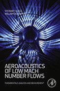
We can of course evaluate the divergence theorem for this new variable and integrate over an infinite region V_∞ bounded only at infinity by the surface S_∞, so

${\displaystyle {\int }_{V_{\infty }}\nabla \cdot \left(\mathbf{v}{H}_s\left(f\right)\right)dV}=-{\displaystyle {\int }_{S_{\infty }}\left(\mathbf{v}{H}_s\left(f\right)\right)\cdot \mathbf{n}dS}$

It follows from Eq. (5.1.6) that

${\displaystyle {\int }_{V_{\infty }}\left(H_s\left(f\right)\nabla \cdot \mathbf{v}+\mathbf{v}\cdot \mathbf{n}\delta \left(f\right)|\nabla f|\right)dV}=-{\displaystyle {\int }_{S_{\infty }}\mathbf{v}\cdot \mathbf{n}dS}$

If we apply the divergence theorem to the first term in the integrand of this equation, then

${\displaystyle {\int }_{V_{\infty }}{H}_s\left(f\right)\left(\nabla \cdot \mathbf{v}\right)dV}={\displaystyle {\int }_{V_o}\left(\nabla \cdot \mathbf{v}\right)dV}=-{\displaystyle {\int }_{S_o+S_{\infty }}\mathbf{v}\cdot \mathbf{n}dS}$

where V_o is the region outside of S_o where f>0, and S_o is the surface of the body where f=0, which may of course be a function of time. It then follows from Eq. (5.1.8) that

${\displaystyle {\int }_{V_{\infty }}\mathbf{v}\cdot \mathbf{n}\delta \left(f\right)|\nabla f|dV}={\displaystyle {\int }_{S_o}\mathbf{v}\cdot \mathbf{n}dS}$

This result is invaluable for the analysis of moving surfaces because the effect of the surface motion is completely defined by the integrand on the left of this expression.

Now let us consider the time derivatives of our new variable vH_s(f), which will be given by

$\frac{\partial \left(\mathbf{v}{H}_s\left(f\right)\right)}{\partial t}=H_s\left(f\right)\frac{\partial \mathbf{v}}{\partial t}+\mathbf{v}\delta \left(f\right)\frac{\partial f}{\partial t}$

For a surface which moves with velocity V it follows that f is a function of $\mathbf{x}-{\displaystyle \int \mathbf{V}dt}$ on the surface and so the chain rule gives

${\left[\frac{\partial f(\mathbf{x}-\int \mathbf{V}dt)}{\partial t}\right]}_{f=0}={\left[-\mathbf{V}\cdot \nabla f\right]}_{f=0}$

then Eq. (5.1.11) is modified to

$\frac{\partial \left(\mathbf{v}{H}_s\left(f\right)\right)}{\partial t}=H_s\left(f\right)\frac{\partial \mathbf{v}}{\partial t}-\mathbf{v}\delta \left(f\right)\left(\mathbf{V}\cdot \mathbf{n}|\nabla f|\right)$

so that the second term on the right is specified in terms of the surface velocity.

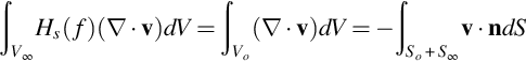
Next consider the material derivative of vH_s, which is given by

$\frac{D\left(\mathbf{v}{H}_s\right)}{Dt}=\frac{D\mathbf{v}}{Dt}{H}_s+\mathbf{v}\frac{Df}{Dt}\delta \left(f\right)$

Using Eq. (5.1.12) we see that

$\frac{Df}{Dt}=\frac{\partial f}{\partial t}+\left(\mathbf{v}\mathbf{.}\mathbf{\nabla }\right)f\mathbf{=}\left(\mathbf{v}-\mathbf{V}\right)\cdot \mathbf{n}|\nabla f|$

For an impermeable boundary the velocity of the fluid normal to the surface is equal to the surface velocity in this direction and so v·n=V·n and it follows that Df/Dt=0. Hence the second term in Eq. (5.1.14), which is only nonzero on the surface, can be eliminated for impermeable surfaces.

Finally, in the next section, we need to consider integrals that include a Green's function. For example,

${\displaystyle {\int }_{V_{\infty }}G\frac{\partial }{\partial y_i}\left(p_{ij}{n}_j\delta \left(f\right)|\nabla f|\right)dV\left(\mathbf{y}\right)}$

which we can expand as

${\displaystyle {\int }_{V_{\infty }}\frac{\partial }{\partial y_i}\left(G{p}_{ij}{n}_j\delta \left(f\right)|\nabla f|\right)dV\left(\mathbf{y}\right)}-{\displaystyle {\int }_{V_{\infty }}\left(p_{ij}{n}_j\delta \left(f\right)|\nabla f|\left)\frac{\partial G}{\partial y_i}dV\right(\mathbf{y}\right)}$

The first of these two integrals can be evaluated using the divergence theorem, but since the only boundary to V_∞ is at infinity where G tends to zero, its net contribution is zero so

${\displaystyle {\int }_{V_{\infty }}G\frac{\partial }{\partial y_i}\left(p_{ij}{n}_j\delta \left(f\right)|\nabla f|\right)dV\left(\mathbf{y}\right)}=-{\displaystyle {\int }_{V_{\infty }}\left(p_{ij}{n}_j\delta \left(f\right)|\nabla f|\left)\frac{\partial G}{\partial y_i}dV\right(\mathbf{y}\right)}$

Similarly for integrands which include time derivatives we can show that, integrating by parts and noting that G is zero when τ=±T, then

${\displaystyle {\int }_{-T}^T{\displaystyle {\int }_{V_{\infty }}G\frac{\partial }{\partial \tau }\left(v_j{n}_j\delta \left(f\right)|\nabla f|\right)dV\left(\mathbf{y}\right)d\tau }}=-{\displaystyle {\int }_{-T}^T{\displaystyle {\int }_{V_{\infty }}\left(v_j{n}_j\delta \left(f\right)|\nabla f|\right)\frac{\partial G}{\partial \tau }dV\left(\mathbf{y}\right)d\tau }}$

These results summarize some of the basic concepts of generalized derivatives. In the next section we will show how they can be used to provide a solution to Lighthill's equation in the presence of moving surfaces.

5.2 The Ffowcs Williams and Hawkings equation

In this section we will consider how the concept of a generalized derivative may be used to obtain the solution to Lighthill's equation in the presence of moving surfaces. We will start by evaluating the continuity and momentum equations in terms of the new variables vH_s, pH_s, and ρH_s which are defined everywhere in an unbounded infinite volume V_∞. To obtain the continuity equation (2.2.6) in terms of the new variables we expand

$\frac{\partial \left({\rho }^{\prime }{H}_s\right)}{\partial t}+\frac{\partial \left(\rho v_i{H}_s\right)}{\partial x_i}=H_s\left(\frac{\partial {\rho }^{\prime }}{\partial t}+\frac{\partial \left(\rho v_i\right)}{\partial x_i}\right)+\left(\left(\rho v_j-{\rho }^{\prime }{V}_j\right)n_j\right)\delta \left(f\right)|\nabla f|$

where ρ′=ρ−ρ_∞. The first term on the right is zero because it is the continuity equation in the region where the flow is defined, and zero outside the flow region because H_s is zero. It follows that it is zero everywhere, so

$\frac{\partial \left({\rho }^{\prime }{H}_s\right)}{\partial t}+\frac{\partial \left(\rho v_i{H}_s\right)}{\partial x_i}=\left(\rho v_j-{\rho }^{\prime }{V}_j\right)n_j\delta \left(f\right)|\nabla f|$

A similar procedure may be applied to the momentum equation given by Eq. (2.3.9), leading to

$\frac{\partial \left(\rho v_i{H}_s\right)}{\partial t}+\frac{\partial \left(\rho v_i{v}_j{H}_s+p_{ij}{H}_s\right)}{\partial x_j}=\left(\rho v_i\left(v_j-V_j\right)+p_{ij}\right)n_j\delta \left(f\right)|\nabla f|$

(where the pressure is defined as gauge pressure as in Chapter 4). We can then obtain a wave equation for the new variable ρ′H_s in exactly the same way we did for Lighthill's equation in Section 4.1. Taking the time derivative of Eq. (5.2.2), the divergence of Eq. (5.2.3) and subtracting gives an equation equivalent to Eq. (4.1.3). Then subtracting ${\partial }^2\left({\rho }^{\prime }{c}_{\infty }^2{H}_s\right)/\partial x_i^2$ from both sides gives

$\begin{array}{c}\frac{{\partial }^2\left({\rho }^{\prime }{H}_s\right)}{\partial t^2}-c_{\infty }^2\frac{{\partial }^2\left({\rho }^{\prime }{H}_s\right)}{\partial x_i^2}=\frac{{\partial }^2\left(T_{ij}{H}_s\right)}{\partial x_i\partial x_j}-\frac{\partial }{\partial x_i}\left(\left(\rho v_i\left(v_j-V_j\right)+p_{ij}\left)n_j\delta \left(f\right)\right|\nabla f\right|\right)\\ +\frac{\partial }{\partial t}\left(\left(\rho v_j-{\rho }^{\prime }{V}_j\right)n_j\delta \left(f\right)|\nabla f|\right)\end{array}$

This is the Ffowcs Williams and Hawkings equation [1], which is an inhomogeneous wave equation that includes the effects of moving surfaces on the right hand side. We can solve this equation using the method of Green's functions as was done in Section 4.2, but since the dependent variable of the wave equation is defined in an unbounded medium, the surface integrals, which appeared in Eq. (4.3.3), are not required and we obtain

$\begin{array}{c}{\rho }^{\prime }\left(\mathbf{x},t\right)c_{\infty }^2{H}_s={\displaystyle {\int }_{-T}^T{\displaystyle {\int }_{V_{\infty }}G\left(\frac{{\partial }^2\left(H_s{T}_{ij}\right)}{\partial y_i\partial y_j}\right)dV\left(\mathbf{y}\right)d\tau }}\\ -{\displaystyle {\int }_{-T}^T{\displaystyle {\int }_{V_{\infty }}G\frac{\partial }{\partial y_i}\left(\left(\rho v_i\left(v_j-V_j\right)+p_{ij}\left)n_j\delta \left(f\right)\right|\nabla f\right|\right)dV\left(\mathbf{y}\right)d\tau }}\\ +{\displaystyle {\int }_{-T}^T{\displaystyle {\int }_{V_{\infty }}G\frac{\partial }{\partial \tau }\left(\left(\rho v_j-{\rho }^{\prime }{V}_j\right)n_j\delta \left(f\right)|\nabla f|\right)dV\left(\mathbf{y}\right)d\tau }}\end{array}$

Using the same procedure employed in deriving Eqs. (4.3.4)–(4.3.6) we can recast the first integral term as

${\displaystyle {\int }_{-T}^T{\displaystyle {\int }_{V_{\infty }}\frac{{\partial }^{2}G}{\partial y_i\partial y_j}\left(T_{ij}{H}_s\right)dV\left(\mathbf{y}\right)d\tau }}$

where the additional surface integral that appears in Eq. (4.3.6) is zero in the present case because of the unbounded domain. We can also convert the second and third terms in Eq. (5.2.5) using the identities established in Eqs. (5.1.18), (5.1.19) to give

$\begin{array}{c}{\rho }^{\prime }\left(\mathbf{x},t\right)c_{\infty }^2{H}_s={\displaystyle {\int }_{-T}^T{\displaystyle {\int }_{V_{\infty }}\frac{{\partial }^{2}G}{\partial y_i\partial y_j}\left(T_{ij}{H}_s\right)dV\left(\mathbf{y}\right)d\tau }}\\ +{\displaystyle {\int }_{-T}^T{\displaystyle {\int }_{V_{\infty }}\left(\left(\rho v_i\left(v_j-V_j\right)+p_{ij}\left)n_j\delta \left(f\right)\right|\nabla f\right|\right)\frac{\partial G}{\partial y_i}dV\left(\mathbf{y}\right)d\tau }}\\ -{\displaystyle {\int }_{-T}^T{\displaystyle {\int }_{V_{\infty }}\left(\left(\rho v_j-{\rho }^{\prime }{V}_j\right)n_j\delta \left(f\right)|\nabla f|\right)\frac{\partial G}{\partial \tau }dV\left(\mathbf{y}\right)d\tau }}\end{array}$

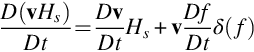
We can obtain the form preferred by Ffowcs Williams for the free field Green's function G=G_o, by noting that, since x and y are fixed,

$\frac{\partial G_o}{\partial y_i}=-\frac{\partial G_o}{\partial x_i}\frac{\partial G_o}{\partial \tau }=-\frac{\partial G_o}{\partial t}$

and thus,

$\begin{array}{c}{\rho }^{\prime }\left(\mathbf{x},t\right)c_{\infty }^2{H}_s=\frac{{\partial }^2}{\partial x_i\partial x_j}{\displaystyle {\int }_{-T}^T{\displaystyle {\int }_{V_{\infty }}\left(T_{ij}{H}_s\right)G_{o}dV\left(\mathbf{y}\right)d\tau }}\\ -\frac{\partial }{\partial x_i}{\displaystyle {\int }_{-T}^T{\displaystyle {\int }_{V_{\infty }}\left(\left(\rho v_i\left(v_j-V_j\right)+p_{ij}\left)n_j\delta \left(f\right)\right|\nabla f\right|\right)G_{o}dV\left(\mathbf{y}\right)d\tau }}\\ +\frac{\partial }{\partial t}{\displaystyle {\int }_{-T}^T{\displaystyle {\int }_{V_{\infty }}\left(\left(\rho v_j-{\rho }^{\prime }{V}_j\right)n_j\delta \left(f\right)|\nabla f|\right)G_{o}dV\left(\mathbf{y}\right)d\tau }}\end{array}$

where partial derivatives have been shifted to the observer variables, as in Eq. (4.3.11). Both these results are given because in some applications it is easier to evaluate the differentials at the source as in Eq. (5.2.6), whereas in other applications the differentials are more accurately applied at the observer location as in Eq. (5.2.7).

Evaluating the second and third integrals in Eq. (5.2.6) using Eq. (5.1.10) converts them to surface integrals

$\begin{array}{c}{\rho }^{\prime }\left(\mathbf{x},t\right)c_{\infty }^2={\displaystyle {\int }_{-T}^T{\displaystyle {\int }_{V_o\left(\tau \right)}\frac{{\partial }^{2}G}{\partial y_i\partial y_j}{T}_{ij}dV\left(\mathbf{y}\right)d\tau }}\\ +{\displaystyle {\int }_{-T}^T{\displaystyle {\int }_{S_o\left(\tau \right)}\frac{\partial G}{\partial y_i}\left(\left(\rho v_i\left(v_j-V_j\right)+p_{ij}\right)n_j\right)dS\left(\mathbf{y}\right)d\tau }}\\ -{\displaystyle {\int }_{-T}^T{\displaystyle {\int }_{S_o\left(\tau \right)}\frac{\partial G}{\partial \tau }\left(\left(\rho v_j-{\rho }^{\prime }{V}_j\right)n_j\right)dS\left(\mathbf{y}\right)d\tau }}\end{array}$

Notice how this result reduces to Curle's equation (4.3.9) when the surfaces are stationary so V=0. It is important to appreciate that this result is not an obvious extension to Curle's theorem because of the change to the momentum flux term and the additional surface source ρ′V_j. Also note how the volume and surface integrals must now be evaluated over moving surfaces, which adds a new level of complexity because the sources are moving relative to the observer, so both y and the propagation distance between the source and the observer will change with emission time.

One of the key simplifications to this result is for an impenetrable surface where the flow velocity normal to the surface equals the surface normal velocity so that v_in_i=V_in_i. This eliminates the momentum flux terms in the second integral and because ρ−ρ′=ρ_∞ the integrand in the third integral reduces to ρ_∞V_in_i giving

$\begin{array}{c}{\rho }^{\prime }\left(\mathbf{x},t\right)c_{\infty }^2={\displaystyle {\int }_{-T}^T{\displaystyle {\int }_{V_o\left(\tau \right)}\frac{{\partial }^{2}G}{\partial y_i\partial y_j}{T}_{ij}dV\left(\mathbf{y}\right)d\tau }}\\ +{\displaystyle {\int }_{-T}^T{\displaystyle {\int }_{S_o\left(\tau \right)}\frac{\partial G}{\partial y_i}{p}_{ij}{n}_{j}dS\left(\mathbf{y}\right)d\tau }}\\ -{\displaystyle {\int }_{-T}^T{\displaystyle {\int }_{S_o\left(\tau \right)}\frac{\partial G}{\partial \tau }{\rho }_{\infty }{V}_j{n}_{j}dS\left(\mathbf{y}\right)d\tau }}\end{array}$

The volume and surface integrals in Eqs. (5.2.8) or (5.2.9) can be evaluated by defining a coordinate system that moves with the surface. Moving coordinates will be denoted by z which is identical to the fixed source coordinate y at time τ_o so for emission times τ>τ_o we have

$\mathbf{y}=\mathbf{z}+{\displaystyle {\int }_{{\tau }_o}^{\tau }\mathbf{V}\left(t^{\prime }\right)d{t}^{\prime }}$

The surface and volume integrals can be evaluated in the moving coordinate system provided we account for the change in the size of the volume and surface elements introduced by this transformation, hence we specify the Jacobians J and K such that dV(y)=JdV(z) and dS(y)=KdS(z). It will be left as an exercise for the reader to show that if surfaces are moving with constant linear or angular velocity then the Jacobians are unity and ∂G/∂y_i=∂G/∂z_i.

Now let us return to Ffowcs Williams' form of these equations given by Eq. (5.2.7). An important application of Eq. (5.2.7) is in propeller or helicopter rotor noise where the surfaces are rotating and translating in an otherwise stationary medium. In this case the free field Green's function is appropriate and we are most concerned with the acoustic far field. The Green's function is given by

$G_o=\frac{\delta \left(t-\tau -r\left(\tau \right)/c_{\infty }\right)}{4\pi r\left(\tau \right)}r\left(\tau \right)=|\mathbf{x}-\mathbf{z}-\left[{\mathbf{U}}_s+\left(\mathbf{z}\times \Omega \right)\right]\left(\tau -{\tau }_o\right)|$

where U_s is the translational velocity of the propeller and Ω is its angular velocity about the origin of z. If we convert the volume integrals to surface integrals we obtain,

$\begin{array}{c}{\rho }^{\prime }\left(\mathbf{x},t\right)c_{\infty }^2=\frac{{\partial }^2}{\partial x_i\partial x_j}{\displaystyle {\int }_{-T}^T{\displaystyle {\int }_{V_{\infty }}{T}_{ij}{G}_{o}dV\left(\mathbf{z}\right)d\tau }}\\ -\frac{\partial }{\partial x_i}{\displaystyle {\int }_{-T}^T{\displaystyle {\int }_{S_o\left(\tau \right)}\left(\left(\rho v_i\left(v_j-V_j\right)+p_{ij}\right)n_j\right)G_{o}dS\left(\mathbf{z}\right)d\tau }}\\ +\frac{\partial }{\partial t}{\displaystyle {\int }_{-T}^T{\displaystyle {\int }_{S_o\left(\tau \right)}\left(\rho v_j-{\rho }^{\prime }{V}_j\right)G_{o}dS\left(\mathbf{z}\right)d\tau }}\end{array}$

Since the Green's function is multiplied into each integrand, we can now perform the time integrations. These are made easier by noting that, with g=t−τ−r(τ)/c_∞,

$\begin{array}{c}{\displaystyle {\int }_{-T}^{T}f\left(\tau \right)\delta \left(g\left(\tau \right)\right)d\tau }={\displaystyle {\int }_{g\left(-T\right)}^{g\left(T\right)}\frac{f\left(\tau \right)\delta \left(g\right)}{\left(\partial g/\partial \tau \right)}\mathit{dg}}\\ ={\left[\frac{f}{\left|\partial g/\partial \tau \right|}\right]}_{g=0}={\left[\frac{f}{\left|-1-\frac{1}{c_{\infty }}\frac{\partial r}{\partial \tau }\right|}\right]}_{\tau ={\tau }^{⁎}}={\left[\frac{f}{\left|1-M_r\right|}\right]}_{\tau ={\tau }^{⁎}}\end{array}$

where M_rc_∞=−∂r/∂τ is the velocity of the source in the direction of the observer, and the correct retarded time τ⁎ is the solution to ${\tau }^{⁎}=t-r\left({\tau }^{⁎}\right)/c_{\infty }$. Thus the Ffowcs Williams Hawkings equation becomes,

$\begin{array}{c}{\rho }^{\prime }\left(\mathbf{x},t\right)c_{\infty }^2{H}_s=\frac{{\partial }^2}{\partial x_i\partial x_j}{\displaystyle {\int }_{V_o}{\left[\frac{T_{ij}}{4\pi r|1-M_r|}\right]}_{\tau =\tau ⁎}dV\left(\mathbf{z}\right)}\\ -\frac{\partial }{\partial x_i}{\displaystyle {\int }_{S_o}{\left[\frac{\left(\rho v_i\left(v_j-V_j\right)+p_{ij}\right)n_j}{4\pi r|1-M_r|}\right]}_{\tau =\tau ⁎}dS}\\ +\frac{\partial }{\partial t}{\displaystyle {\int }_{S_o}{\left[\frac{\left(\rho v_j-{\rho }^{\prime }{V}_j\right)n_j}{4\pi r|1-M_r|}\right]}_{\tau =\tau ⁎}dS}\end{array}$

In this result the integrals are carried out over the moving surface at the correct emission time, and then the acoustic field is differentiated to obtain the final result.

In the acoustic far field, where the sound is the only disturbance and the sound waves are propagating radially away from the source, the space and time derivatives can be exchanged. This is simply a reflection of the fact that the change of the acoustic pressure in time experienced at a fixed point is the same as the change in space multiplied by the sound speed. To verify this for moving surfaces, we evaluate the gradient of the free field Green's function defined in Eq. (5.2.11) as

$\begin{array}{c}\frac{\partial G_o}{\partial x_i}=\frac{\partial }{\partial x_i}\left(\frac{\delta \left(g\right)}{4\pi r\left(\tau \right)}\right)=\frac{\partial r}{\partial x_i}\left(\frac{\partial g}{\partial r}\frac{\partial \delta \left(g\right)}{\partial g}\frac{1}{4\pi r\left(\tau \right)}-\frac{\delta \left(g\right)}{4\pi r^2\left(\tau \right)}\right)\\ =\frac{x_i-y_i}{r}\left(\frac{-1}{c_{\infty }}\frac{\partial \delta \left(g\right)}{\partial t}\frac{1}{4\pi r\left(\tau \right)}-\frac{\delta \left(g\right)}{4\pi r^2\left(\tau \right)}\right)=-\frac{x_i-y_i}{r}\left(\frac{1}{c_{\infty }}\frac{\partial G_o}{\partial t}+\frac{G_o}{r\left(\tau \right)}\right)\end{array}$

In the acoustic far field where |x|≫|y| the derivatives of the Green's function can therefore be approximated by

$\frac{\partial G_o}{\partial x_i}\approx -\frac{x_i}{\left|\mathbf{x}\right|}\left(\frac{1}{c_{\infty }}\frac{\partial G_o}{\partial t}\right)$

The approximation may be applied to both the dipole and quadrupole terms in Eq. (5.2.13) giving the far field approximation for impermeable surfaces, as

$\begin{array}{c}{\rho }^{\prime }\left(\mathbf{x},t\right)c_{\infty }^2\approx \frac{x_i{x}_j}{\left|\mathbf{x}\right|{}^2}\frac{1}{c_{\infty }^2}\frac{{\partial }^2}{\partial t^2}{\displaystyle {\int }_{V_o}{\left[\frac{T_{ij}}{4\pi \left|\mathbf{x}\right||1-M_r|}\right]}_{\tau =\tau ⁎}dV\left(\mathbf{z}\right)}\\ +\frac{x_i}{\left|\mathbf{x}\right|}\frac{1}{c_{\infty }}\frac{\partial }{\partial t}{\displaystyle {\int }_{S_o}{\left[\frac{p_{ij}{n}_j}{4\pi \left|\mathbf{x}\right||1-M_r|}\right]}_{\tau =\tau ⁎}dS\left(\mathbf{z}\right)}\\ +\frac{\partial }{\partial t}{\displaystyle {\int }_{S_o}{\left[\frac{{\rho }_{\infty }{V}_j{n}_j}{4\pi \left|\mathbf{x}\right||1-M_r|}\right]}_{\tau =\tau ⁎}dS\left(\mathbf{z}\right)}\end{array}$

The result shows that for propeller or rotor noise there are three terms of importance. The first is the quadrupole term whose strength depends on T_ij and is the sound radiated by both turbulence and flow distortions such as shock waves that are associated with the blades. The second is the dipole source term that is controlled by the surface loading p_ij. Finally, we have a term ρ_∞V_jn_j that depends only on the blade surface velocity and the density at the observer. This is a volume displacement source and is only nonzero if the observer “sees” a time varying surface velocity at emission time. This source is zero for an object in linear motion traveling toward the observer, but nonzero for a rotating blade which continuously changes direction relative to the observer. All the integrands are evaluated at emission time τ=τ⁎=t−r(τ⁎)/c_∞ and so for moving sources, the emitted time history and the observed time history are distorted relative to each other by the motion. We can shift the time differentials from the observed field onto the source terms using

$\frac{\partial }{\partial t}=\frac{\partial {\tau }^{⁎}}{\partial t}\frac{\partial }{\partial \tau }=\frac{1}{1-M_r}\frac{\partial }{\partial \tau }$

which introduces an extra factor of (1−M_r)⁻¹ for each time derivative in Eq. (5.2.15). A physical interpretation of this result is that the motion of the source compresses the time history as the source moves towards the observer, and this dramatically increases the radiated sound, especially when the relative Mach number M_r approaches one. Also note that the integrals become singular when M_r=1, and so special care needs to be exercised when evaluating these source terms for propellers or rotors with supersonic tip speeds. We will discuss this issue in more detail in Chapter 16 when we review rotor noise.

5.3 Moving sources

To illustrate some of the subtleties of the results given above we will evaluate the acoustic field from a moving source using Eq. (5.2.13). Consider an acoustically compact surface that is moving through a stationary fluid with constant speed U_s in the x₁ direction. We will assume that the sound from turbulence in the fluid is negligible compared to the sound from the surface sources, and that the size of the surface is small compared to the propagation distance to the observer. If the source is acoustically compact, then the differences in retarded time from different points on the surface can be ignored and we can approximate the source to observer distance r as |x−y^(c)|. Here y^(c) is the centroid of the surface, at the correct retarded time, in the fixed reference frame, corresponding to z=0 in the moving frame. Therefore, from Eq. (5.2.11),

$r\left(\tau \right)=|\mathbf{x}-{\mathbf{U}}_s\tau |$

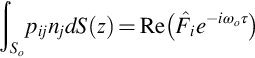
where we have taken the time origin of the surface motion τ_o to be zero. The surface terms in Eq. (5.2.13) can then be simplified by taking the terms that depend on the propagation distance outside of the surface integrals giving

$\begin{array}{c}{\rho }^{\prime }\left(\mathbf{x},t\right)c_{\infty }^2\approx -\frac{\partial }{\partial x_i}{\left[\frac{1}{4\pi r|1-M_r|}\left\{{\displaystyle {\int }_{S_o}{p}_{ij}{n}_{j}dS\left(\mathbf{z}\right)}\right\}\right]}_{\tau =\tau ⁎}\\ +\frac{\partial }{\partial t}{\left[\frac{1}{4\pi r|1-M_r|}\left\{{\displaystyle {\int }_{S_o}{\rho }_{\infty }{V}_j{n}_{j}dS\left(\mathbf{z}\right)}\right\}\right]}_{\tau =\tau ⁎}\end{array}$

Since V_j=(U_s,0,0) is constant on the surface the last term integrates to zero and the only contribution comes from the dipole term. The surface integral of p_ijn_j in that term is the net force applied to the fluid by the surface. For modeling purposes we take this as being a harmonic source in the frame of reference moving with the surface, with vector amplitude ${\hat{F}}_i$, defined as

${\displaystyle {\int }_{S_o}{p}_{ij}{n}_{j}dS\left(z\right)=\mathrm{R}\mathrm{e}\left({\hat{F}}_i{e}^{-i{\omega }_o\tau }\right)}$

so that the acoustic field is given by

${\rho }^{\prime }\left(\mathbf{x},t\right)c_{\infty }^2\approx -\mathrm{R}\mathrm{e}\left(\frac{\partial }{\partial x_i}{\left[\frac{{\hat{F}}_i{e}^{-i{\omega }_o\tau }}{4\pi r|1-M_r|}\right]}_{\tau =\tau ⁎}\right)$

The retarded time is evaluated by solving the equation t=τ+r(τ)/c_∞ or

$t-\tau ={\left({\left(x_1-U_s\tau \right)}^2+x_2^2+x_3^2\right)}^{1/2}/c_{\infty }$

The retarded times τ=τ⁎ can be obtained in terms of the observer time by squaring this equation and solving the resultant quadratic equation giving

${\tau }^{⁎}=\frac{\left(c_{\infty }t-M{x}_1\right)\pm \sqrt{{\left(x_1-U_{s}t\right)}^2+\left(1-M^2\right)\left(x_2^2+x_3^2\right)}}{c_{\infty }\left(1-M^2\right)}$

where M=U_s/c_∞. There are two possible solutions to this equation, but it is also constrained by the causality condition, which requires that t>τ. For subsonic source speeds where M<1 the only option is to choose the negative sign on the square root in Eq. (5.3.3) (this is readily verifiable by setting x₂=x₃=0). However, for supersonic source speeds, two real solutions are possible if ${\left(x_1-U_{s}t\right)}^2>\left(M^2-1\right)\left(x_2^2+x_3^2\right)$. To illustrate this Fig. 5.3A shows a series of wave fronts emitted from a source that is moving subsonically, and Fig. 5.3B shows the wave fronts for a source moving supersonically.

These figures highlight the physics of the problem. For the subsonic case (Fig. 5.3A), the wave fronts spread out from the source, but as the source moves the center of the wavefronts changes. This causes an apparent contraction of the acoustic wavelength for an observer ahead of the source, and an apparent increase in frequency of the signal. For an observer behind the source, the apparent wavelength is increased and the observed frequency of the signal is decreased. In the far field the retarded time equation can be approximated using the far field approximation discussed in Section 3.6 with y₁=U_sτ, so

$r\left(\tau \right)\approx \left|\mathbf{x}\right|-x_1{U}_s\tau /\left|\mathbf{x}\right|+\cdots$

The velocity of the source in the direction of the observer is U_r=U_sx₁/|x| and the source Mach number in the direction of the observer is M_r=U_r/c_∞. The far field approximation applied to Eq. (5.3.2) then gives

$t-\tau \approx \left|\mathbf{x}\right|/c_{\infty }-M_r\tau \mathrm{or}\tau \approx \left(t-\left|\mathbf{x}\right|/c_{\infty }\right)/\left(1-M_r\right)$

leading to the approximation of Eq. (5.3.1) as

$\begin{array}{c}{\rho }^{\prime }\left(\mathbf{x},t\right)c_{\infty }^2\approx -\mathrm{R}\mathrm{e}\left(\frac{\partial }{\partial x_i}\left[\frac{{\hat{F}}_i{e}^{-i{\omega }_o\left(t-\left|\mathbf{x}\right|/c_{\infty }\right)/\left(1-M_r\right)}}{4\pi \left|\mathbf{x}\right||1-M_r|}\right]\right)\\ \approx \mathrm{R}\mathrm{e}\left(\frac{-i{\omega }_o{x}_i{\hat{F}}_i{e}^{-i{\omega }_o\left(t-\left|\mathbf{x}\right|/c_{\infty }\right)/\left(1-M_r\right)}}{4\pi c_{\infty }\left|\mathbf{x}\right|{}^2{\left(1-M_r\right)}^2}+O\left(\left|\mathbf{x}\right|{}^{-2}\right)\right)\end{array}$

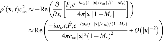
where near field terms of order |x|⁻² have been ignored. This shows that the apparent frequency at the observer is multiplied by a factor (1−M_r)⁻¹ giving an increase of frequency when the source approaches the observer, and M_r is positive, and a reduction of frequency as the source moves away from the observer, and M_r is negative. This is called the Doppler frequency shift and is well known in many applications. We also note that the source has a dipole directivity given by x_i/|x| as expected, but there is also a directivity caused by the source motion. In this example the source is said to have two powers of Doppler amplification because there is a factor of (1−M_r)² on the bottom line of Eq. (5.3.5). This can significantly increase the levels as the source approaches the observer and reduce the levels as the source moves away.

When the source is moving supersonically as illustrated in Fig. 5.3B the situation is quite different. The source is now moving faster than the acoustic waves it generates and so it cannot be heard as it approaches the observer. This is to be expected from the solution to the retarded time equation (5.3.3) because the argument of the square root is negative if ${\left(x_1-U_{s}t\right)}^2>\left(M^2-1\right)\left(x_2^2+x_3^2\right)$. To expand on this, we note that the term (x₁−U_st) is the source position at reception time t (see Fig. 5.4) and for a real solution to Eq. (5.3.3) we require

$\frac{\left|x_1-U_{s}t\right|}{\sqrt{x_2^2+x_3^3}}=cot\mu >\sqrt{M^2-1}$

where μ is the angle of the observer to the path of the source evaluated at reception time, as shown in Fig. 5.4. We can rearrange this inequality so that it reads

$\mu <{sin}^{-1}\left(\frac{1}{M}\right)$

where sin⁻¹(1/M) defines the angle of the Mach cone caused by the source motion, which is illustrated by the leading boundary of the waves in Fig. 5.3B. Inside the Mach cone we see that two wave fronts reach the same point at the same time, and this corresponds to the two possible solutions to the retarded time equation (5.3.3) when the argument of the square root is positive. An interesting point is that the propagation time for the wave front that originated from the source after it has passed the observer is shorter than the propagation time for the wave front originating from the source before it passed the observer, and hence the signal emitted by the source is both Doppler shifted and reversed in time!

The characteristics of sources moving at speed are important when we consider rotating sources such as propellers, helicopter rotors, and wind turbines, which will be considered in Part 4 of the text. We will leave further discussion of this topic until that time.

5.4 Sources in a free stream

In many applications we are interested in the sound radiation from a uniform flow over a stationary object. Examples include model testing in wind tunnels, the flow in ducts, flow over large surfaces such as aircraft fuselages, and perhaps most importantly CFD calculations in body fixed coordinates. In each case there is a uniform steady flow at large distances from the region of turbulence that causes the sound and this contradicts the assumption, made in both Lighthill's acoustic analogy and the Ffowcs Williams and Hawkings equation that the medium is at rest at infinity. We showed in Section 4.2 that, in a uniform flow, the Lighthill stress tensor needed to be modified to only include the unsteady perturbations relative to the uniform flow, and that the acoustic propagation was determined by the convected wave equation. In principle, we can solve this modified equation using the techniques described earlier in this chapter using solutions to the convected wave equation. However, a simpler approach is often possible if we work in a frame of reference moving with the uniform flow, in which the medium appears stationary and the source and the observer are seen to be moving upstream at the flow speed. This approach is accommodated by modifying the results of this chapter to include a moving source and observer and by referencing flow velocity perturbations to the free stream.

An important application of this theory is to ducted fan noise where the sources are stationary or rotating next to stationary surfaces. The acoustic propagation is most readily addressed in this case by using the convected wave equation. It is possible to model this propagation by using a Green's function that satisfies the boundary conditions on the wall of the duct. We therefore need a formulation that will correctly allow for moving sources in a uniform flow that is bounded by stationary surfaces.

First consider the solution to Lighthill's wave equation in a frame of reference moving with the uniform flow velocity U^(∞)=(U_∞,0,0). The velocity perturbations relative to the moving frame of reference are given by w, so the velocity in the fixed frame is v=U^(∞)+w. Lighthill's stress tensor is defined in the moving frame as

$T_{ij}^{\prime }=\rho w_i{w}_j+\left(p-p_{\infty }\right){\delta }_{ij}-\left(\rho -{\rho }_{\infty }\right)c_{\infty }^2{\delta }_{ij}-{\sigma }_{ij}$

Also the velocity of the surface relative to the fixed frame is $V_j-U_j^{\left(\infty \right)}$. Eq. (5.2.8) can then be written, for the positions x′ and y′ in the moving frame as

$\begin{array}{c}{\rho }^{\prime }\left({\mathbf{x}}^{\mathbf{\prime }},t\right)c_{\infty }^2={\displaystyle {\int }_{-T}^T{\displaystyle {\int }_{V_o\left(\tau \right)}\frac{{\partial }^{2}G}{\partial y_i^{\prime }\partial y_j^{\prime }}{T}_{ij}^{\prime }dV\left({\mathbf{y}}^{\mathbf{\prime }}\right)d\tau }}\\ +{\displaystyle {\int }_{-T}^T{\displaystyle {\int }_{S_o\left(\tau \right)}\frac{\partial G}{\partial y_i^{\prime }}\left(\left(\rho w_i\left(w_j-V_j+U_j^{\left(\infty \right)}\right)+p_{ij}\right)n_j\right)dS\left({\mathbf{y}}^{\mathbf{\prime }}\right)d\tau }}\\ -{\displaystyle {\int }_{-T}^T{\displaystyle {\int }_{S_o\left(\tau \right)}\frac{\partial G}{\partial \tau }\left((\rho w_j-{\rho }^{\prime }\left(V_j-U_j^{\left(\infty \right)}\right)n_j\right)dS\left({\mathbf{y}}^{\mathbf{\prime }}\right)d\tau }}\end{array}$

We wish to change this result to give a solution at the points x and y, which are the observer and source locations in the fixed frame of reference. As part of this we need to replace the Green's function. In the moving frame where no free stream is observed, the Green's function is a solution to the inhomogeneous wave equation,

$\frac{1}{c_{\infty }^2}\frac{{\partial }^{2}G}{\partial {\tau }^2}-\frac{{\partial }^{2}G}{\partial {y^{\prime }}_i^2}=\delta \left({\mathbf{x}}^{\mathbf{\prime }}-{\mathbf{y}}^{\mathbf{\prime }}\right)\delta \left(t-\tau \right)$

The Green's function in the fixed frame, G_e(x,t|y,τ), will be related to G by straightforward translation of the coordinates,

$G\left({\mathbf{x}}^{\mathbf{\prime }},t|{\mathbf{y}}^{\mathbf{\prime }},\tau \right)=G_e\left(\mathbf{x}+{\mathbf{U}}^{\left(\infty \right)}t,t|\mathbf{y}+{\mathbf{U}}^{\left(\infty \right)}\tau ,\tau \right)$

and thus

$\frac{\partial G}{\partial y_i^{\prime }}=\frac{\partial G_e}{\partial y_i}\mathrm{and}\frac{\partial G}{\partial \tau }=\frac{\partial G_e}{\partial \tau }+U_i^{\left(\infty \right)}\frac{\partial G_e}{\partial y_i}=\frac{D_{\infty }{G}_e}{D\tau }$

where D_∞/Dτ is the free stream convective derivative, introduced in Eq. (4.2.9). Applying these conversions to Eq. (3.9.2) we see that the fixed frame Green's function must be a solution to the equation,

$\frac{1}{c_{\infty }^2}\frac{D_{\infty }^2{G}_e}{D\tau }-{\nabla }^2{G}_e=\delta \left(t-\tau \right)\delta \left(\mathbf{x}-\mathbf{y}\right)$

and so we obtain

$\begin{array}{c}{\rho }^{\prime }\left(\mathbf{x},t\right)c_{\infty }^2={\displaystyle {\int }_{-T}^T{\displaystyle {\int }_{V_o\left(\tau \right)}\frac{{\partial }^2{G}_e}{\partial y_i\partial y_j}{T}_{ij}^{\prime }dV\left(\mathbf{y}\right)d\tau }}\\ +{\displaystyle {\int }_{-T}^T{\displaystyle {\int }_{S_o\left(\tau \right)}\frac{\partial G_e}{\partial y_i}\left(\left(\rho w_i\left(w_j-V_j+U_j^{\left(\infty \right)}\right)+p_{ij}\right)n_j\right)dS\left(\mathbf{y}\right)d\tau }}\\ -{\displaystyle {\int }_{-T}^T{\displaystyle {\int }_{S_o\left(\tau \right)}\frac{D_{\infty }{G}_e}{D\tau }\left((\rho w_j-{\rho }^{\prime }\left(V_j-U_j^{\left(\infty \right)}\right)n_j\right)dS\left(\mathbf{y}\right)d\tau }}\end{array}$

An important application of Eq. (5.4.3) is in CFD calculations or surface flows in which the surfaces are stationary and the medium is in uniform motion at infinity. In this case V=0 and the nonpenetration boundary condition on the surfaces require that (U^(∞)+w)·n=0 on all the surfaces. The integrand of the last integral in Eq. (5.4.3) then reduces to ${\rho }_{\infty }{U}_j^{\left(\infty \right)}{n}_j{D}_{\infty }{G}_e/D\tau$ which does not vary with time and so makes no contribution to the acoustic field. A similar reduction can be made to the second integral in Eq. (5.4.3) and, neglecting viscous stresses as we did in Section 4.5, gives

$\begin{array}{l}{\rho }^{\prime }\left(\mathbf{x},t\right)c_{\infty }^2={\displaystyle {\int }_{-T}^T{\displaystyle {\int }_{S_o}\frac{\partial G_e}{\partial y_i}{p}^{\prime }{n}_{i}dS\left(\mathbf{y}\right)d\tau }}+{\displaystyle {\int }_{-T}^T{\displaystyle {\int }_{V_o}\frac{{\partial }^2{G}_e}{\partial y_i\partial y_j}{T}_{ij}^{\prime }dV\left(\mathbf{y}\right)d\tau }}\\ \end{array}$

where p′=p−p_∞. This result is identical to Eq. (4.5.1), which was the result for a stationary medium, the differences being that the Green's function must satisfy the convected wave equation (5.4.2), and that the Lighthill stress tensor depends on ρw_iw_j.

5.5 Ffowcs Williams and Hawkings surfaces

One of the most useful applications of the formulas given above is in the calculation of the acoustic far field from detailed numerical simulations of a flow within a limited region. Recent advances in computational methods have enabled the accurate calculation of many time varying flows of practical interest. Provided the Mach number is not too high, these solutions provide both the unsteady flow and the acoustics inside a computational grid, but the computational domain is limited by the size of the computer, and usually cannot be extended to the acoustic far field. Furthermore, increasing the size of the computational domain soon becomes a wasteful exercise because wave propagation outside the flow is well understood and modeled by the linear wave equation. The purpose of a Ffowcs Williams and Hawkings (FWH) surface is to provide a far field solution to the wave equation given accurate numerical calculations on a surface which bounds the source region. It is assumed that the calculations are accurate inside the source region and that they accurately capture the compressible flow fluctuations and the acoustic waves, so that the FWH surface may be arbitrarily located within the numerical domain. This is important because the numerical calculations at the edges of the computational domain may be adversely influenced by numerical boundary conditions, so the FWH surface is usually placed inside the numerical domain in a region where there is confidence in the calculations. However, it is preferable, but not absolutely necessary, to choose the surface so that the Lighthill stress tensor does not contribute to the far field in the region outside the FWH surface. Then Eq. (5.2.13) can be used without the quadrupole source terms to give the acoustic field as

$\begin{array}{c}{\rho }^{\prime }\left(\mathbf{x},t\right)c_{\infty }^2{H}_s=-\frac{\partial }{\partial x_i}{\displaystyle {\int }_{S_o}{\left[\frac{\left(\rho v_i\left(v_j-V_j\right)+p_{ij}\right)n_j}{4\pi r|1-M_r|}\right]}_{\tau =\tau ⁎}dS}\\ +\frac{\partial }{\partial t}{\displaystyle {\int }_{S_o}{\left[\frac{\left(\rho v_j-{\rho }^{\prime }{V}_j\right)n_j}{4\pi r|1-M_r|}\right]}_{\tau =\tau ⁎}dS}\end{array}$

This result implies that if we know the flow quantities on S_o (which may be moving relative to the observer) then we can calculate the acoustic far field everywhere outside the computational domain. Obviously we need to check that the surface is in the right place and that the dropping of the quadrupole term is a good approximation. As shown by Brentner and Farassat [2], this can be done by recalculating the results on a slightly different surface and checking that the far field is independent of surface location. Notice that in this formula we need to know the mass flux, the surface stress, and the momentum flux on the surface. These variables are available in an unsteady compressible flow calculation, but the incorrect result will be obtained from an incompressible flow calculation because the acoustic waves which couple with the far field will be missing unless the surface is very small compared to the acoustic wavelength. For a rotating source, such as a helicopter rotor, the steady flow in blade based coordinates can be used as the input to Eq. (5.5.1) to give a time varying far field. This can include detached shock waves that are local to the blade and inside the computational domain. When the blade encounters an unsteady flow event, such as a blade vortex interaction, then obviously the time varying surface quantities must be used.

To apply Eq. (5.5.1), it is necessary to calculate the integrand at the emission time for of each element of the FWH surface. This can require significantly more accurate time computations on the surface than would be required in the acoustic far field. It can therefore be advantageous to move the time derivatives in Eq. (5.5.1) inside the integrand. For the acoustic far field this can be done by using

$\frac{\partial }{\partial x_i}\approx -\frac{x_i}{\left|\mathbf{x}\right|}\frac{1}{c_{\infty }}\frac{\partial }{\partial t}$

and Eq. (5.2.16) to give the form used by Farassat [3]

$\begin{array}{l}{\rho }^{\prime }\left(\mathbf{x},t\right)c_{\infty }^2{H}_s\approx \frac{1}{c_{\infty }}{\displaystyle {\int }_{S_o}{\left[\frac{x_i}{4\pi \left|\mathbf{x}\right|{}^2{\left(1-M_r\right)}^2}\left\{\frac{\partial L_i}{\partial \tau }+\frac{L_i}{\left(1-M_r\right)}\frac{\partial M_r}{\partial \tau }\right\}\right]}_{\tau =\tau ⁎}dS}\hfill \\ +{\displaystyle {\int }_{S_o}{\left[\frac{1}{4\pi \left|\mathbf{x}\right|{\left(1-M_r\right)}^2}\left\{\frac{\partial q}{\partial \tau }+\frac{q}{\left(1-M_r\right)}\frac{\partial M_r}{\partial \tau }\right\}\right]}_{\tau =\tau ⁎}dS}\end{array}$

with

$\begin{array}{c}{L}_i=\left(\rho v_i\left(v_j-V_j\right)+p_{ij}\right)n_{j}q=\left(\rho v_j-{\rho }^{\prime }{V}_j\right)n_j\hfill \end{array}$

where terms of order |x|⁻² have been dropped. The source terms on the surface can now be readily evaluated and differentiated in source time, and then propagated to the far field. There is still a requirement to match the observer time and the emission time, but this can be done with less restrictive requirements on numerical accuracy if the differentials are evaluated in source time.

In conclusion, the approach described above is very attractive because it overcomes one of the main limitations of Lighthill's theory. Specifically, it moves the application of Lighthill's equation to the region where it is unambiguously defined, and allows all the processes which are taking place to be determined by the numerical code inside the FWH surface. However, the accuracy of the result depends on the accuracy of the calculations on the surface. It is only the surface perturbations that couple to the acoustic field which are needed, and unfortunately these may be a small part of the net motion. The signal to noise ratio of the integrands in Eq. (5.5.2) is therefore determined by the ratio of the propagating waves to the numerical noise, not the ratio of the absolute fluctuations to the numerical noise. In later chapters we will discuss how we can discriminate the propagating and nonpropagating parts of the surface source terms, and show that it is the disturbances with supersonic phase speeds on the FWH surface (relative to the observer) which are the most important.

5.6 Incompressible flow estimates of acoustic source terms

In the previous section we discussed the use of FWH surfaces to couple CFD calculations over a finite volume to the acoustic far field. This requires that the acoustic waves are correctly defined on the FWH surface and this will only be the case if they are computed using the compressible equations of motion. At low Mach numbers the CFD grid required for a compressible calculation stretches the limits of computational capabilities. In general, a FWH surface surrounding a computational domain of arbitrary size cannot be used with the output from an incompressible flow calculation. However, it has been shown by Wang et al. [4] that some valuable results can be obtained at low Mach numbers if the output of an incompressible flow calculation is used to specify the source terms in Lighthill's acoustic analogy, provided the volume integral is broken down into source regions that are very small compared to the acoustic wavelength.

With the flow computed incompressibly, the speed of sound used in the application of Lighthill's equation can be taken as constant so that acoustic density perturbations are directly related to the acoustic pressure fluctuations as $p-p_{\infty }=\left(\rho -{\rho }_{\infty }\right)c_{\infty }^2$. Lighthill's stress tensor can then be approximated by ρ_ow_iw_j where w_i is the flow perturbation relative to a constant velocity $U_j^{\left(\infty \right)}$ at the inflow boundary of the computational domain (see Section 5.4). Acoustic radiation from low Mach number turbulent flows without surfaces present is normally of very low level, and so the surface source terms are usually of primary interest. In almost all cases the viscous terms on the surfaces are assumed to be negligible. The surface source term in Eq. (5.4.4) is then determined by the surface pressure. If the surface is acoustically compact and all parts of the turbulent flow are within a fraction of an acoustic wavelength from the surface, then the surface pressure can be approximated by the pressure fluctuations that are obtained from the incompressible CFD calculation. However, if the surface is large compared to the acoustic wavelength, then this approximation is invalid because the acoustic waves on the surface are not included. For example, the sound radiated by the trailing edge of an airfoil is often modeled by a semi-infinite flat plate that extends to the upstream limit of the computational domain. As we will show below, the far field sound from turbulence near the corner of a large flat plate will scale quite differently from the sound from an acoustically compact surface, and this limits the use of the surface hydrodynamic pressure for acoustic calculations.

An alternative approach, used by Wang et al. [4], is to combine the calculated Lighthill's stress tensor with a tailored Green's function, as in Eq. (4.5.2). This eliminates the need to evaluate the surface integral and the far field sound is calculated directly from the unsteady flow. Unfortunately, tailored Green's functions are only available for a limited set of idealized shapes. An alternative numerical approach, developed by Khalighi et al. [5], is to numerically calculate the surface pressure from the volume source terms using a boundary element method. This calculation is most easily done in the frequency domain and implies that the pressure term in Eq. (4.5.4) (or the Fourier transform of Eq. 5.4.4) is solved for the unknown surface pressure $\tilde{p}$ with the volume sources defined from an incompressible CFD calculation. The resulting integral equation is of course singular because the Green's function is singular when the source point and observer point merge, but the approach described in Section 4.6 can be used to eliminate the singularity. The size of the surface is in principle not limited, but boundary integral methods are only applicable to closed surfaces, and so some approximation must be used to close semi-infinite surfaces without introducing additional scattering. This is a three step approach: first an unsteady incompressible CFD code is used to calculate the turbulent flow, and then a compressible boundary element method is used to numerically calculate the surface pressure from the volume source terms in Lighthill's analogy. The final step is to calculate the acoustic far field from the surface pressure on the boundary and the volume sources. However, both these methods assume that Lighthill's analogy can be used to calculate the pressure perturbations within the flow and, as we will discuss below, this limits their application to low Mach number flows.

The physical element that is missing from these approaches is the back reaction of the acoustic waves on the unsteady flow near corners and edges. For example, acoustic feedback loops that occur in cavities and in laminar boundary layers will not be simulated because they are often caused by acoustic rather than hydrodynamic feedback. A classical example is a singing airfoil where the instabilities in a laminar boundary layer close to the leading edge of an airfoil grow with distance downstream and produce the regular shedding of eddies from the trailing edge. Potential flow and acoustic perturbations produced by the shedding are then felt upstream near the leading edge where they serve to originate and organize the boundary layer instability.

The process is controlled by the upstream feedback, which can be caused by either potential flow perturbations or acoustic waves that originate at the trailing edge. The amplitude of the potential flow perturbations scale with 1/r², where r is the distance from the source of the disturbance. In contrast acoustic perturbations, which are initially much weaker, scale with distance as 1/r. At distances that are of the order of an acoustic wavelength, the acoustic disturbances can dominate because their decay with distance is much less than the decay of potential perturbations. If acoustic propagation is left out of the calculation, as it is in an incompressible flow code, then the feedback that disturbs the upstream laminar boundary layer will be much weaker and may not initiate a sufficient disturbance to trigger the feedback loop. This issue is not limited to low frequencies because the feedback loop is nonlinear, and so instabilities at very high frequencies can cause significant flow excursions at low frequencies that would not be modeled correctly by an incompressible flow calculation.

Finally, it must be pointed out that Lighthill's formulation was never intended for calculations within the flow, and this in itself can be a limitation when the mean flow Mach number is increased above about 0.3. To illustrate this point, consider Lighthill's source term when there is a significant distortion of the mean flow from its uniform inflow value. If we define the mean flow as $U_i=U_i^{\left(\infty \right)}+\mathrm{\Delta }{U}_i$ where $U_i^{\left(\infty \right)}$ is constant then the velocity relative to the constant flow is w_i=ΔU_i+u_i and the source term in Lighthill's wave equation can be broken down into linear and nonlinear terms as follows:

$\begin{array}{ll}\rho w_i{w}_j=& \underset{\mathrm{Steady}\mathrm{flow}}{\underbrace{{\rho }_{\infty }\mathrm{\Delta }{U}_i\mathrm{\Delta }{U}_j}}+\underset{\mathrm{Linear}\mathrm{terms}}{\underbrace{{\rho }_{\infty }\mathrm{\Delta }{U}_i{u}_j+{\rho }_{\infty }{u}_i\mathrm{\Delta }{U}_j+{\rho }^{\prime }\mathrm{\Delta }{U}_i\mathrm{\Delta }{U}_j}}+\underset{\mathrm{Nonlinear}\mathrm{terms}}{\underbrace{{\rho }_{\infty }{u}_i{u}_j+{\rho }^{\prime }{u}_i{u}_j}}\hfill \end{array}$

The important point is that when there is significant distortion of the mean flow then terms that are linear in the perturbation velocity will dominate the source terms if ΔU≫u. For flows over obstructions that include stagnation points or for weakly turbulent inflows over streamlined shapes, the linear terms will dominate. However, if that is the case then we cannot ignore the term ρ′ΔU_iΔU_j which depends on the acoustic variable ρ′, and so is not a source term. It is also not included in incompressible flow calculations. This term represents the refraction of sound waves by the mean flow and should be part of the wave operator. This is one of the inherent limitations of Lighthill's analogy but will only have a small impact if ${\rho }^{\prime }\Delta U_i\Delta U_j\ll {\rho }^{\prime }{c}_{\infty }^2$, which suggests the limit ΔU/c_∞<0.3. To address this limitation a theory is required that does not include the acoustic variable in the source term. In the next chapter we will address this issue by assuming that the turbulence is sufficiently weak that the linear terms in Eq. (5.6.1) dominate the production of sound.