Chapter 7

Dynamic Range Control

The dynamic range of a signal is defined as the logarithmic ratio of maximum to minimum signal amplitude and is given in decibels. The dynamic range of an audio signal lies between 40 and 120 dB. The combination of level measurement and adaptive signal level adjustment is called dynamic range control. Dynamic range control of audio signals is used in many applications to match the dynamic behavior of the audio signal to different requirements. While recording, dynamic range control protects the AD converter from overload or is employed in the signal path to optimally use the full amplitude range of a recording system. For suppressing low-level noise, so-called noise gates are used so that the audio signal is passed through only from a certain level onwards. While reproducing music and speech in a car, shopping center, restaurant or disco the dynamics have to match the special noise characteristics of the environment. Therefore the signal level is measured from the audio signal and a control signal is derived which then changes the signal level to control the loudness of the audio signal. This loudness control is adaptive to the input level.

7.1 Basics

Figure 7.1 shows a block diagram of a system for dynamic range control. After measuring the input level X_dB(n), the output level Y_dB(n) is affected by multiplying the delayed input signal x(n) by a factor g(n) according to

The delay of the signal x(n) compared with the control signal g(n) allows predictive control of the output signal level. This multiplicative weighting is carried out with corresponding attack and release time. Multiplication leads, in terms of a logarithmic level representation of the corresponding signals, to the addition of the weighting level G_dB(n) to the input level X_dB(n), giving the output level

Figure 7.1 System for dynamic range control.

7.2 Static Curve

The relationship between input level and weighting level is defined by a static level curve G_dB(n) = f(X_dB(n)). An example of such a static curve is given in Fig. 7.2. Here, the output level and the weighting level are given as functions of the input level.

Figure 7.2 Static curve with the parameters (LT = limiter threshold, CT = compressor threshold, ET = expander threshold and NT = noise gate threshold).

With the help of a limiter, the output level is limited when the input level exceeds the limiter threshold LT. All input levels above this threshold lead to a constant output level. The compressor maps a change of input level to a certain smaller change of output level. In contrast to a limiter, the compressor increases the loudness of the audio signal. The expander increases changes in the input level to larger changes in the output level. With this, an increase in the dynamics for low levels is achieved. The noise gate is used to suppress low-level signals, for noise reduction and also for sound effects like truncating the decay of room reverberation. Every threshold used in particular parts of the static curve is defined as the lower limit for limiter and compressor and upper limit for expander and noise gate.

In the logarithmic representation of the static curve the compression factor R (ratio) is defined as the ratio of the input level change ΔP_I to the output level change ΔP_O:

With the help of Fig. 7.3 the straight line equation Y_dB(n) = CT + R⁻¹(X_dB(n) − CT) and the compression factor

are obtained, where the angle β is defined as shown in Fig. 7.2. The relationship between the ratio R and the slope S can also be derived from Fig. 7.3 and is expressed as

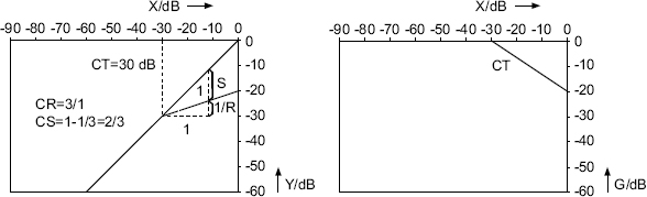
Figure 7.3 Compressor curve (compressor ratio CR/slope CS).

Typical compression factors are

The transition from logarithmic to linear representation leads, from (7.4), to

where and are the linear levels and c_T denotes the linear compressor threshold. Rewriting (7.8) gives the linear output level

as a function of input level. The control factor g(n) can be calculated by the quotient

With the help of tables and interpolation methods, it is possible to determine the control factor without taking logarithms and antilogarithms. The implementation described as follows, however, makes use of the logarithm of the input level and calculates the control level G_dB(n) with the help of the straight line equation. The antilogarithm leads to the value f(n) which gives the control factor g(n) with corresponding attack and release time (see Fig. 7.1).

7.3 Dynamic Behavior

Besides the static curve of dynamic range control, the dynamic behavior in terms of attack and release times plays a significant role in sound quality. The rapidity of dynamic range control depends also on the measurement of PEAK and RMS values [McN84, Sti86].

7.3.1 Level Measurement

Level measurements [McN84] can be made with the systems shown in Figs 7.4 and 7.5. For PEAK measurement, the absolute value of the input is compared with the peak value x_PEAK(n). If the absolute value is greater than the peak value, the difference is weighted with the coefficient AT (attack time) and added to (1 − AT) · x_PEAK(n − 1). For this attack case |x(n)|>x_PEAK(n − 1) we get the difference equation (see Fig. 7.4)

with the transfer function

If the absolute value of the input is smaller than the peak value |x(n)|≤x_PEAK(n − 1) (the release case), the new peak value is given by

with the release time coefficient RT. The difference signal of the input will be muted by the nonlinearity such that the difference equation for the peak value is given according to (7.13). For the release case the transfer function

is valid. For the attack case the transfer function (7.12) with coefficient AT is used and for the release case the transfer function (7.14) with the coefficient RT. The coefficients (see Section 7.3.3) are given by

where the attack time t_a and the release time t_r are given in milliseconds (T_S sampling interval). With this switching between filter structures one achieves fast attack responses for increasing input signal amplitudes and slow decay responses for decreasing input signal amplitudes.

Figure 7.4 PEAK measurement.

Figure 7.5 RMS measurement (TAV = averaging coefficient).

The computation of the RMS value

over N input samples can be achieved by a recursive formulation. The RMS measurement shown in Fig. 7.5 uses the square of the input and performs averaging with a first-order low-pass filter. The averaging coefficient

is determined according to the time constant calculation discussed in Section 7.3.3, where t_M is the averaging time in milliseconds. The difference equation is given by

with the transfer function

7.3.2 Gain Factor Smoothing

Attack and release times can be implemented by the system shown in Fig. 7.6 [McN84]. The attack coefficient AT or release coefficient RT is obtained by comparing the input control factor and the previous one. A small hysteresis curve determines whether the control factor is in the attack or release state and hence gives the coefficient AT or RT. The system also serves to smooth the control signal. The difference equation is given by

with k = AT or k = RT, and the corresponding transfer function leads to

Figure 7.6 Implementing attack and release time or gain factor smoothing.

7.3.3 Time Constants

If the step response of a continuous-time system is

then sampling (step-invariant transform) the step response gives the discrete-time step response

The Z-transform leads to

With the definition of attack time t_a = t₉₀ − t₁₀, we derive

The relationship between attack time t_a and the time constant τ of the step response is obtained as follows:

Hence, the pole is calculated as

A system for implementing the given step response is obtained by the relationship between the Z-transform of the impulse response and the Z-transform of the step response:

The transfer function can now be written as

with the pole z_∞ = e^{−2.2T_S/t_a} adjusting the attack, release or averaging time. For the coefficients of the corresponding time constant filters the attack case is given by (7.15), the release case by (7.16) and the averaging case by (7.18). Figure 7.7 shows an example where the dotted lines mark the t₁₀ and t₉₀ time.

7.4 Implementation

The programming of a system for dynamic range control is described in the following sections.

7.4.1 Limiter

The block diagram of a limiter is presented in Fig. 7.8. The signal x_PEAK(n) is determined from the input with variable attack and release time. The logarithm to the base 2 of this peak signal is taken and compared with the limiter threshold. If the signal is above the threshold, the difference is multiplied by the negative slope of the limiter LS. Then the antilogarithm of the result is taken. The control factor f(n) obtained is then smoothed with a first-order low-pass filter (SMOOTH). If the signal x_PEAK(n) lies below the limiter threshold, the signal f(n) is set to f(n) = 1. The delayed input x(n − D₁) is multiplied by the smoothed control factor g(n) to give the output y(n).

7.4.2 Compressor, Expander, Noise Gate

The block diagram of a compressor/expander/noise gate is shown in Fig. 7.9. The basic structure is similar to the limiter. In contrast to the limiter, the logarithm of the signal x_RMS(n) is taken and multiplied by 0.5. The value obtained is compared with three thresholds in order to determine the operating range of the static curve. If one of the three thresholds is crossed, the resulting difference is multiplied by the corresponding slope (CS, ES, NS) and the antilogarithm of the result is taken. A first-order low-pass filter subsequently provides the attack and release time.

Figure 7.7 Attack and release behavior for time-constant filters.

Figure 7.8 Limiter.

Figure 7.9 Compressor/expander/noise gate.

Figure 7.10 Limiter/compressor/expander/noise gate.

7.4.3 Combination System

A combination of a limiter that uses PEAK measurement, and a compressor/expander/noise gate that is based on RMS measurement, is presented in Fig. 7.10. The PEAK and RMS values are measured simultaneously. If the linear threshold of the limiter is crossed, the logarithm of the peak signal x_PEAK(n) is taken and the upper path of the limiter is used to calculate the characteristic curve. If the limiter threshold is not crossed, the logarithm of the RMS value is taken and one of the three lower paths is used. The additive terms in the limiter and noise gate paths result from the static curve. After going through the range detector, the antilogarithm is taken. The sequence f(n) is smoothed with a SMOOTH filter in the limiter case, or weighted with corresponding attack and release times of the relevant operating range (compressor, expander or noise gate). By limiting the maximum level, the dynamic range is reduced. As a consequence, the overall static curve can be shifted up by a gain factor. Figure 7.11 demonstrates this with a gain factor equal to 10 dB. This static parameter value is directly included in the control factor g(n).

Figure 7.11 Shifting the static curve by a gain factor.

As an example, Fig. 7.12 illustrates the input x(n), the output y(n) and the control factor g(n) of a compressor/expander system. It is observed that signals with high amplitude are compressed and those with low amplitude are expanded. An additional gain of 12 dB shows the maximum value of 4 for the control factor g(n). The compressor/expander system operates in the linear region of the static curve if the control factor is equal to 4. If the control factor is between 1 and 4, the system operates as a compressor. For control factors lower than 1, the system works as an expander (3500 < n < 4500 and 6800 < n < 7900). The compressor is responsible for increasing the loudness of the signal, whereas the expander increases the dynamic range for signals of small amplitude.

7.5 Realization Aspects

7.5.1 Sampling Rate Reduction

In order to reduce the computational complexity, downsampling can be carried out after calculating the PEAK/RMS value (see Fig. 7.13). As the signals x_PEAK(n) and x_RMS(n) are already band-limited, they can be directly downsampled by taking every second or fourth value of the sequence. This downsampled signal is then processed by taking its logarithm, calculating the static curve, taking the antilogarithm and filtering with corresponding attack and release time with reduced sampling rate. The following upsampling by a factor of 4 is achieved by repeating the output value four times. This procedure is equivalent to upsampling by a factor of 4 followed by a sample-and-hold transfer function.

Figure 7.12 Signals x(n), y(n) and g(n) for dynamic range control.

The nesting and spreading of partial program modules over four sampling periods is shown in Fig. 7.14. The modules PEAK/RMS (i.e. PEAK/RMS calculation) and MULT (delay of input and multiplication with g(n)) are performed every input sampling period. The number of processor cycles for PEAK/RMS and MULT are denoted by Z1 and Z3 respectively. The modules LD (X), CURVE, 2^x and SMO have a maximum of Z2 processor cycles and are processed consecutively in the given order. This procedure is repeated every four sampling periods. The total number of processor cycles per sampling period for the complete dynamics algorithm results from the sum of all three modules.

Figure 7.13 Dynamic system with sampling rate reduction.

Figure 7.14 Nesting technique.

7.5.2 Curve Approximation

Besides taking logarithms and antilogarithms, other simple operations like comparisons and addition/multiplication occur in calculating the static curve. The logarithm of the PEAK/RMS value is taken as follows:

First, the mantissa is normalized and the exponent is determined. The function ld(M) is then calculated by a series expansion. The exponent is simply added to the result.

The logarithmic weighting factor G and the antilogarithm 2^G are given by

Here, E is a natural number and M is a fractional number. The antilogarithm 2^G is calculated by expanding the function 2^−M in a series and multiplying by 2^−E. A reduction of computational complexity can be achieved by directly using log and antilog tables.

7.5.3 Stereo Processing

For stereo processing, a common control factor g(n) is needed. If different control factors are used for both channels, limiting or compressing one of the two stereo signals causes a displacement of the stereo balance. Figure 7.15 shows a stereo dynamic system in which the sum of the two signals is used to calculate a common control factor g(n). The following processing steps of measuring the PEAK/RMS value, downsampling, taking logarithm, calculating static curve, taking antilog attack and release time and upsampling with a sample-and-hold function remain the same. The delay (DEL) in the direct path must be the same for both channels.

Figure 7.15 Stereo dynamic system.

7.6 Java Applet – Dynamic Range Control

The applet shown in Fig. 7.16 demonstrates dynamic range control. It is designed for a first insight into the perceptual effects of dynamic range control of an audio signal. You can adjust the characteristic curve with two control points. You can choose between two predefined audio files from our web server (audio1.wav or audio2.wav) or your own local wav file to be processed [Gui05].

Figure 7.16 Java applet – dynamic range control.

7.7 Exercises

1. Low-pass Filtering for Envelope Detection

Generally, envelope computation is performed by low-pass filtering the input signal's absolute value or its square.

1. Sketch the block diagram of a recursive first-order low-pass H(z) = λ/[(1 − (1 − λ)z⁻¹)].
2. Sketch its step response. What characteristic measure of the envelope detector can be derived from the step response and how?
3. Typically, the low-pass filter is modified to use a non-constant filter coefficient λ. How does λ depend on the signal? Sketch the response to a rect signal of the low-pass filter thus modified.

2. Discrete-time Specialties of Envelope Detection

Taking absolute value or squaring are non-linear operations. Therefore, care must be taken when using them in discrete-time systems as they introduce harmonics the frequency of which may violate the Nyquist bound. This can lead to unexpected results, as a simple example illustrates. Consider the input signal .

1. Sketch x(n), |x(n)| and x²(n) for different values of φ.
2. Determine the value of the envelope after perfect low-pass filtering, i.e. averaging, |x(n)|. Note: As the input signal is periodical, it is sufficient to consider one period, e.g.

   

3. Similarly, determine the value of the envelope after averaging x²(n).

3. Dynamic Range Processors

Sketch the characteristic curves mapping input level to output level and input level to gain for and describe briefly the application of:

1. limiter;
2. compressor;
3. expander;
4. noise gate.

References

[Gui05] M. Guillemard, C. Ruwwe, U. Zölzer: J-DAFx – Digital Audio Effects in Java, Proc. 8th Int. Conference on Digital Audio Effects (DAFx-05), pp. 161–166, Madrid, 2005.

[McN84] G. W. McNally: Dynamic Range Control of Digital Audio Signals, J. Audio Eng. Soc., Vol. 32, pp. 316–327, 1984.

[Sti86] E. Stikvoort: Digital Dynamic Range Compressor for Audio, J. Audio Eng. Soc., Vol. 34, pp. 3–9, 1986.