
The network architecture is very simple. An input image, of size 784 pixels, is stochastically corrupted, and then it is dimensionally reduced by an encoding network layer. The reduction step is from 784 to 256 pixels.
In the decoding phase, we prepare the network for output, re-changing the original image size from 256 to 784 pixels.
As usual, we start loading all the necessary libraries to our implementation:
import numpy as np
import tensorflow as tf
import matplotlib.pyplot as plt
from tensorflow.examples.tutorials.mnist import input_data
Set the basic network parameters:
n_input    = 784
n_hidden_1 = 256
n_hidden_2 = 256
n_output   = 784
We also set the session's parameters:
epochs     = 110
batch_size = 100
disp_step  = 10
We build the training and test sets. We again use the input_data feature imported from the tensorflow.examples.tutorials.mnist library present in the installation package:
print ("PACKAGES LOADED")
mnist = input_data.read_data_sets('data/', one_hot=True)
trainimg   = mnist.train.images
trainlabel = mnist.train.labels
testimg    = mnist.test.images
testlabel  = mnist.test.labels
print ("MNIST LOADED")
Let's define a placeholder variable for the input images. The data type is set to float and the shape is set to [None, n_input]. The None parameter means that the tensor may hold an arbitrary number of images, and the size per image is n_input:
x = tf.placeholder("float", [None, n_input])
Next, we have a placeholder variable for the true labels associated with the images that were input in the placeholder variable x. The shape of this placeholder variable is [None, n_output], which means it may hold an arbitrary number of labels, and each label is a vector of length n_output, which is 10 in this case:
y = tf.placeholder("float", [None, n_output])
To reduce overfitting, we'll apply a dropout before the encoding and decoding procedure, so we must define a placeholder for the probability that a neuron's output is kept during the dropout:
dropout_keep_prob = tf.placeholder("float")
On these definitions, we fix the weights and network's biases:
weights = {
    'h1': tf.Variable(tf.random_normal([n_input, n_hidden_1])),
    'h2': tf.Variable(tf.random_normal([n_hidden_1, n_hidden_2])),
    'out': tf.Variable(tf.random_normal([n_hidden_2, n_output]))
}
biases = {
    'b1': tf.Variable(tf.random_normal([n_hidden_1])),
    'b2': tf.Variable(tf.random_normal([n_hidden_2])),
    'out': tf.Variable(tf.random_normal([n_output]))
}
Weights and biases are chosen using tf.random_normal, which returns random values with a normal distribution.
The encoding phase takes as its input an image from the MNIST dataset, and then performs the data compression, applying a matrix multiplication operation:
encode_in = tf.nn.sigmoid
          (tf.add(tf.matmul
                  (x, weights['h1']),
                  biases['b1']))
encode_out = tf.nn.dropout
             (encode_in, dropout_keep_prob)
In the decoding phase, we apply the same procedure:
decode_in = tf.nn.sigmoid
          (tf.add(tf.matmul
                  (encode_out, weights['h2']),
                  biases['b2']))
The over-fitting reduction is made by a dropout procedure:
decode_out = tf.nn.dropout(decode_in,
                           dropout_keep_prob)
Finally, we are ready to build the prediction tensor, y_pred:
y_pred = tf.nn.sigmoid
         (tf.matmul(decode_out,
                    weights['out']) +
          biases['out'])
We then define a cost measure that is used to guide the variables optimization procedure:
cost = tf.reduce_mean(tf.pow(y_pred - y, 2))
We will minimize the cost function, using the RMSPropOptimizer class:
optmizer = tf.train.RMSPropOptimizer(0.01).minimize(cost)
Finally, we can initialize the defined variables:
init = tf.initialize_all_variables()
Set TensorFlow's running session:
with tf.Session() as sess:
    sess.run(init)
    print ("Start Training")
    for epoch in range(epochs):
        num_batch  = int(mnist.train.num_examples/batch_size)
        total_cost = 0.
        for i in range(num_batch):
For each training epoch, we select a smaller batch set from the training dataset:
            batch_xs, batch_ys =
                      mnist.train.next_batch(batch_size)
Here is the focal point: we randomically corrupt the batch_xs set using the random function by the numpy package previously imported:
            batch_xs_noisy = batch_xs +
                             0.3*np.random.randn(batch_size, 784)
We use these sets to feed the execution graph, and then to run the session (sess.run):
            feeds = {x: batch_xs_noisy,
                     y: batch_xs,
                     dropout_keep_prob: 0.8}
            sess.run(optmizer, feed_dict=feeds)
            total_cost += sess.run(cost, feed_dict=feeds)
Every 10 epochs, the average cost value will be shown:
        if epoch % disp_step == 0:
            print ("Epoch %02d/%02d average cost: %.6f"
                   % (epoch, epochs, total_cost/num_batch))
Finally, we start to test the trained model:
print ("Start Test")
To make this, we randomically select an image from the test set:
            randidx   = np.random.randint
                               (testimg.shape[0], size=1)
            orgvec    = testimg[randidx, :]
            testvec   = testimg[randidx, :]
            label     = np.argmax(testlabel[randidx, :], 1)
            print ("Test label is %d" % (label))
            noisyvec = testvec + 0.3*np.random.randn(1, 784)
We then run the trained model on the selected image:
            outvec = sess.run(y_pred,feed_dict={x: noisyvec,
                                           dropout_keep_prob: 1})
As we'll see, the following plotresult function will display the original image, the noisy image, and the predicted image:
            plotresult(orgvec,noisyvec,outvec)
            print ("restart Training")
Running the session, we should see a result like the following:
PACKAGES LOADED
Extracting data/train-images-idx3-ubyte.gz
Extracting data/train-labels-idx1-ubyte.gz
Extracting data/t10k-images-idx3-ubyte.gz
Extracting data/t10k-labels-idx1-ubyte.gz
MNIST LOADED
Start Training
For the sake of brevity, we only report the results after 10 epochs and after 100 epochs:
Epoch 00/100 average cost: 0.212313
Start Test
Test label is 6
The following are the original and the noisy images (the number 6, as you can see):

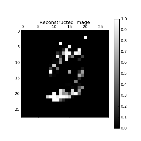
The following shows a poorly reconstructed image:
After 100 epochs, we have a better result:
Epoch 100/100 average cost: 0.018221
Start Test
Test label is 9
Again, the original and the noisy images:

Followed by a good reconstructed image:
