In the previous section, we showed how to access and manipulate the MNIST dataset. In this section, we will see how to address the classification problem of handwritten digits via the TensorFlow library.

We'll apply the concepts taught to build more models of neural networks in order to assess and compare the results of the different approaches followed. The first feed-forward network architecture that will be implemented is represented in the following figure:

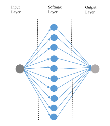
The hidden layer (or softmax layer) of the network consists of 10 neurons, with a softmax transfer function. Remember that it is defined so that its activation is a set of positive values with total sum equal to 1; this means that the j^th value of the output is the probability that j is the class that corresponds with the network input.

Let's see how to implement our neural network model.

The first thing to do is import the necessary libraries and prepare the data for our model:

import tensorflow as tf 
import mnist_data 
 
logs_path = 'log_simple_stats_softmax' 
batch_size = 100 
learning_rate = 0.5 
training_epochs = 10 
 
mnist = mnist_data.read_data_sets("data") 
 

Now let's move on to defining the network model.

The input network consists of a set of images extracted from the MNIST datasets; each image has a size of 28x28 pixels:

X = tf.placeholder(tf.float32, [None, 28, 28, 1],name="input") 

The problem is assigning a probability value for each of the possible classes of membership, that is, the digits from 0 to 9. The corresponding output describes a probability distribution from which we can provide a prediction about the value tested. The output network will be contained in the following placeholder, a tensor of 10 elements:

Y_ = tf.placeholder(tf.float32, [None, 10]) 

The weights take into account the size of the hidden layer (10 neurons) and the input size. The value of the weights must vary at each iteration of the calculation, for which they are defined by the following variable:

 W = tf.Variable(tf.zeros([784, 10]))  

The matrix weight is W [784, 10] where 784 = 28x28.

Let's flatten the images into a single line of pixels; the number -1 in the shape definition means the only possible dimension that will preserve the number of elements:

XX = tf.reshape(X, [-1, 784]) 

In a similar way, we define the biases of the network, the effect of which is to control the translatory motion of the trigger relative to the origin of the input signals. Formally, the bias has a role, not different from the weights, which act as an intensity regulator of the emitted/received signals.

The bias tensor is therefore a variable tensor:

b = tf.Variable(tf.zeros([10])) 

Also the size (=10) is equal to the total number of neurons of the hidden layer.

The input, weight, and bias tensors are sized to define the evidence parameter that quantifies if a certain image belongs to a particular class:

 evidence = tf.matmul(XX, W) + b  

The neural network has only one hidden layer, composed of 10 neurons. Using the feed-forward network definition we know that all neurons at the same level must have the same activation function.

In this model, the activation function is the softmax function, it converts the evidence into probabilities of belonging to each of the 10 possible classes:

 Y = tf.nn.softmax(evidence,name="output")  

The Y output matrix will be formed of 100 rows and 10 columns.

To train our model and to determine if we have a good one, we must define a metric. Indeed, the next goal is to get values for the W and b tensors that minimize the value of a metric and indicate how bad the implemented model is.

Different metrics calculate the degree of error between the desired output and the computed outputs obtained from the training data. The most common error measure is the mean squared error; however, there is some research out there that suggests using other metrics to a neural network like this.

In this example, we use the so-called cross_entropy error function. It is defined as follows:

 cross_entropy = -tf.reduce_mean(Y_ * tf.log(Y)) * 1000.0  

We minimize the error function using the gradient descent algorithm:

 train_step = tf.train.GradientDescentOptimizer(0.005). 
                                           minimize(cross_entropy)  

Here, we have set the learning rate equal to 0.005.

We will have a correct prediction if the Y network output and the desired output Y_are equal:

 correct_prediction = tf.equal(tf.argmax(Y, 1),
                              tf.argmax(Y_, 1))

The correct_prediction variable allows defining the accuracy of the implemented model:

 accuracy = tf.reduce_mean(tf.cast(correct_prediction, 
                                  tf.float32))  

We define the summaries that we want to analyze with TensorBoard:

tf.summary.scalar("cost", cross_entropy)
tf.summary.scalar("accuracy", accuracy)
summary_op = tf.summary.merge_all()

Finally, implemented model is, we must build a session that will take place in the training and testing step:

with tf.Session() as sess:
    sess.run(tf.global_variables_initializer())
    writer = tf.summary.FileWriter(logs_path, 
                                    graph=tf.get_default_graph()) 

The network's training procedure is iterative. It slightly modifies for each learning cycle (or epoch) the synaptic weights by using a selected subset (or batch set):

     for epoch in range(training_epochs): 

It slightly modifies for each learning cycle or epoch the synaptic weights by using a selected set:

       batch_count = int(mnist.train.num_examples/batch_size) 

The selected sets are respectively batch_x e batch_y:

        for i in range(batch_count): 
            batch_x, batch_y = mnist.train.next_batch(batch_size) 

They will be used by the feed_dict statement to feed the network during the training procedure.

At each cycle:

• The weights are modified to minimize the error function.
• The results are added to the summaries using the following writer.add_summary statement:

            _, summary = sess.run([train_step, summary_op],
                                  feed_dict={X: batch_x,
                                             Y_: batch_y}) 
            writer.add_summary(summary,
                               epoch * batch_count + i) 
            print "Epoch: ", epoch 

Finally, we can test the model and evaluate its accuracy:

    print "Accuracy: ", accuracy.eval
          (feed_dict={X: mnist.test.images, 
                      Y_: mnist.test.labels}) 
    print "done"  

After testing the network, we can, while remaining within the session, run the network model on a single image. For example, we can randomly choose via the randint function, a picture from the mnist.test database:

num = randint(0, mnist.test.images.shape[0])  
img = mnist.test.images[num]  

So, we can use the implemented classifier on the selected image:

 classification = sess.run(tf.argmax(Y, 1), feed_dict={X: [img]})   

The arguments of the sess.run function are respectively the output and the input of the network. The tf.argmax(Y, 1) function returns the maximum index value for the Y tensor, which is the image we are looking for, the next argument, feed_dict={X: [img]}, allows us to feed the network with the selected image.

Finally, we display the results, that is, the predicted label and the effective label:

print 'Neural Network predicted', classification[0]  
print 'Real label is:', np.argmax(mnist.test.labels[num])  

The execution is shown in the following snippet. As you can see, after loading the MNIST data, the training epochs are displayed until the ninth:

>>> 
Loading data/train-images-idx3-ubyte.mnist 
Loading data/train-labels-idx1-ubyte.mnist 
Loading data/t10k-images-idx3-ubyte.mnist 
Loading data/t10k-labels-idx1-ubyte.mnist 
Epoch:  0 
Epoch:  1 
Epoch:  2 
Epoch:  3 
Epoch:  4 
Epoch:  5 
Epoch:  6 
Epoch:  7 
Epoch:  8 
Epoch:  9  

Then we display the model's accuracy:

Accuracy:  0.9246 
done 
 
The predicted and real label: 
 
Neural Network predicted 6 
Real label is: 6 
>>>  

After running the model, we can analyze the execution phases of the executions by using TensorBoard.