3

Machine Learning Methods for Genomic Applications

Have you ever wondered how YouTube recommends videos to you, banks detect fraudulent activity and send notifications to you, or Gmail filters the spam messages from your inbox? These are just a few examples of how the world of business is currently using machine learning (ML). The field of ML has impacted numerous areas of modern society and is responsible for some of the most significant improvements in technologies such as self-driving cars, exploring the galaxy, predictions for disease outbreaks, and so on. The enormous growth in ML is primarily driven by its huge success in solving real-world business problems in healthcare, finance, e-commerce, agriculture, life sciences, pharmaceuticals, and biotechnology. The life sciences and biotechnology industries are huge and diverse with many subsectors. Very popular fields are drug discovery and manufacturing, therapeutics, diagnostics, genomics, and so on.

The field of genomics has seen massive growth in the past few years because of advancements in sequencing technologies that have pushed genomic data in the wave of big data. ML techniques, with their ability to analyze large-scale data, can turn this complex genomic data into biological insights that can in turn convert into useful products. ML algorithms have been widely used in biology and genomics to apply to complex multi-dimensional datasets for the building of predictive models to solve complex biological problems such as disorder risk prediction, mental illness prediction, diagnosis, treatment, and so on. This chapter introduces the main ML algorithms and libraries that are commonly used in genomic data analysis. By the end of the chapter, you will know what supervised and unsupervised ML methods are, understand the most common ML algorithms and libraries for genomics, and know when and how to use them. You will know how to build a predictive model using genomics data and be aware of the challenges encountered by ML algorithms for genomics and potential solutions for addressing the same.

As such, here are the contents of this chapter:

• Genomics big data
• Supervised and unsupervised ML
• ML for genomics
• An ML use case for genomics—Disease prediction
• ML challenges in genomics

Technical requirements

Let’s understand the technical requirements for the different Python packages and other ML libraries that are needed to apply ML in genomics in this chapter.

Python packages

The following are some common Python packages that every data scientist and genomic researcher uses for not only genomic analysis for any kind of data analysis.

Pandas

Pandas is one of the most popular data analysis tools in Python. Pandas do not need an introduction as it is part and parcel of every data scientist’s tool. The great thing about Pandas is it contains all the functions and methods to support data analysis irrespective of the type of data. It’s also super easy to install Pandas, which you can do by simply entering pip install pandas in your terminal. Then, you can include import pandas as pd in your Python script, which you will see later in the chapter.

Matplotlib

We will be using Matplotlib, a very popular Python library for visualization. It is one of the easiest libraries to install and use. To install Matplotlib, simply run pip install matplotlib in your terminal. Then, you can include import matplotlib.pyplot as plt in your Python script, which you will see later in the hands-on section of this chapter.

Seaborn

Seaborn is another visualization Python library that we will use in this chapter because of its easy-to-use functionalities for plotting. Again, as with any other Python package, it is easy to install (pip install seaborn) and easy to include in Python scripting (import seaborn as sns).

ML libraries

An ML library is a compilation of functions and routines that are readily available to use without building from scratch. These are an essential part of ML for any field, and they help save time and effort in writing complex code. Furthermore, they also solve complex problems such as data manipulation, text processing, scientific computation, and so on. They simplify the task of performing ML because of their ability to support a variety of ML algorithms. Some of the ML libraries, based on their popularity among ML practitioners and enthusiasts all around the world, include scikit-learn, Keras, PyTorch, TensorFlow, Armadillo, mlpack, and so on. Despite their popularity, building ML models is not trivial as it requires a good understanding and background in data science. For this chapter, we will use scikit-learn.

scikit-learn

scikit-learn is a Python package written for the sole purpose of doing ML and is one of the most popular ML libraries used by data scientists. It has a rich collection of ML algorithms, extensive tutorials, good documentation, and most importantly excellent user community. For this introductory chapter, we will use scikit-learn for developing ML models in Python. Wherever applicable, we will use the scikit-learn 1.0.2 version, and we will look at separate ways of installing scikit-learn in the subsequent chapters.

Genomics big data

Genomics is the study of the function, structure, and evolution of genomes in living organisms. A genome is the blueprint of an organism that has a complete set of DNA, including genes and other intergenic regions. Genes are the basic components of DNA, and they play an important role in inheritance. The field of genomics got mainstream attention after the completion of human genome sequencing in 2003. The human genome project catapulted the field of genomics and it transformed medicine, giving birth to the modern biotechnology industry. Genomics got another push with the introduction of Next-Generation Sequencing (NGS) in the early 2000s, which enabled researchers and scientists to generate massive amounts of data, leading to scientific breakthroughs.

Genomic data has gained a lot of attention in the last decade because of the incredible progress it has made in precision genomics, genomic medicine, drug development, therapeutics, and so on. For example, since the first SARS-CoV-2 (the causative organism of COVID-19) genome was sequenced in December 2019, we have had around 3,035 SARS-CoV-2 genomes sequenced up to May 2022 (https://nextstrain.org/ncov/gisaid/global/all-time), which enabled companies such as Moderna to quickly develop boosters based on the sequence of the variants. These technological advancements in genome sequencing have enabled scientists to create and store that massive data to drive biomedical breakthroughs. For example, a lot of effort has been put into the generation of deep datasets such as The Cancer Genome Atlas (TCGA, 2014), the Encyclopedia of DNA Elements (ENCODE, 2012), GenBank from the National Center for Biotechnology Information (NCBI, 1988), and so on.

Big data is a term that is used to refer to datasets that are larger in size and complexity in terms of type compared to traditional data generation methods.

While genomic big data has enabled life sciences and biotechnology industries to make informed business decisions, this continuous generation of big data has put several constraints on the collection, acquisition, storage, analysis, and sharing of data. In addition, it is estimated that there will be between 2 and 40 exabytes (EB) of genomics data generated in the next decade (https://www.ncbi.nlm.nih.gov/pmc/articles/PMC4494865/).

But thanks to ML, we can now translate this genomic big data into actionable insights that can be applied for research and scientific innovation.

Supervised and unsupervised ML

The goal of ML is to develop and deploy computational algorithms that can automatically learn and improve from experience without human interference to perform a particular task. But how does it work? It does so by first “learning” knowledge from experience from the input data and using that knowledge to make predictions on unseen data. As such, the crux of ML is the learning problem in which machines learn from real-world data, improve from experience, extract patterns, construct models, and predict the outcomes of unseen data.

Depending on the type of data and the tasks to perform, ML algorithms can be broadly divided into supervised, semi-supervised, and unsupervised methods. Supervised methods learn patterns from examples with labels (for example, “diseased” or “not diseased”) and are then used to predict future events or labels from unseen data (Figure 3.1). Unsupervised methods, in contrast, don’t have the luxury of labels, and they rely on examples only to find patterns in the data and create groups (Figure 3.1). Semi-supervised methods combine both supervised and unsupervised methods, using patterns in the unlabeled data and using those to improve the prediction power of labels. Semi-supervised methods are not as popular as the other two approaches and so we will not discuss them in this chapter.

Figure 3.1 – Supervised versus unsupervised ML

Let’s discuss these supervised and unsupervised learning methods with some examples here and in the latter part of the section.

Supervised ML

Supervised ML, as the name suggests, is a class of ML methods that rely on the labels provided during the training of a computer algorithm along with the features from the input data. In other words, it is a type of ML that learns a mapping from input to a set of outcomes for quantitative or categorical values in the training set. This process of learning is called "modeling". The observed value of the variable can be represented by a dimensional matrix of elements where N is the number of observations (for example, number of genes or number of patients/samples) and M is the number of features (for example, single nucleotide polymorphisms (SNPs) or gene expressions values). is an N-dimensional vector of output variables assuming continuous or categorical values. But how do the models know how to learn the mapping from the input to output or modeling is a common question among beginners, but fortunately, we have a lot of information on this process. But before we go into deeper details of supervised ML, let’s look at the different types of supervised ML methods.

Types of supervised ML

Supervised ML methods can be mainly divided into regression and classification based on the most common use cases. A regression model predicts a continuous value (Figure 3.2). Regression-based supervised ML methods employ parametric or non-parametric methods to map the associations of features to lables that are either quantitative or continuous (for example, the amount of gene expression). Several ML algorithms are currently available for performing regression tasks (Figure 3.2). On the other hand, in classification-based supervised ML methods, the output class is specified by a qualitative or discrete or categorical label (for example, type of gene— protein-coding or non-coding) with no explicit ordering (Figure 3.2). The different algorithms for classification tasks are shown in Figure 3.2. Classification models are divided into two different types: binary classification and multiclass classification. As the name suggests, binary classification models output a value from a class consisting of two values—for example, whether a particular DNA sequence is a “gene” or “not gene”. Multiclass classification models, on the other hand, output a value from a class that contains more than two values—for example, a model that classifies either the 5’untranslated region (5’UTR) or coding sequence (CDS) or 3'untranslated region (3'UTR):

Figure 3.2 – Types of supervised ML

How do supervised ML methods work?

At the core of these supervised ML models are optimization methods, which are generally meant for minimizing a loss function. A loss function takes the predicted values and the values corresponding to the real data value and outputs how different they are. For example, in the case of linear regression models, the difference between the predicted methylation value and the original values of the labels’ methylation for samples is considered as “loss”. The lower the loss, the better the model. During model training, supervised methods try to learn the structure of the data to predict a value. Let’s understand this further:

• The mapping function maps a predictor variable from a given sample to the response variable or labels. The response variable is also called the dependent variable. Then, the predictions are simply the output of the mapping function. The variables in the input are also called independent variables, explanatory variables, or features. The output of the mapping function is then compared to the original target value and loss is calculated. If the loss is high, then the model is modified until the loss is zero or minimal.
• The mapping functions also have parameters that help map input data to the predicted values. The optimization works on the parameters and tries to minimize the difference between the predicted output and the original value. This is the main idea of a cost function for regression, which is slightly different from a classification model, but the idea is the same.
• Finally, we need an evaluation method that informs of the predictions of a mapping function. Some of the well-known regression algorithms are root-mean-square error (RMSE), mean absolute error (MAE), R-Squared, and so on.

The key ingredients of a supervised ML algorithm can be summarized are as follows:

1. Define how to represent a mapping function into a model for the machine to understand. This requires two things:
   1. The first is to convert each input data or sample into a set of features or attributes that describe the purpose
   2. The second is to pick a learning model (regression, in the case of continuous labels, and classification, in the case of discrete labels) that learns the system
2. Devise a loss function to optimize the difference between the predictions and the observed values. After converting the problem into a mapping problem, the step is choosing the right cost function that can calculate the difference between the predicted output and the original output.
3. Apply a mathematical optimization method to find the best parameter values in relation to the loss function. Train the chosen model iteratively until we find a model that best fits the data (loss is minimal) by tuning the parameters.
4. Apply an evaluation method that defines some metrics or scores for the prediction of the mapping function.

Let’s next move on to unsupervised ML.

Unsupervised ML

While supervised ML methods aim to predict the output given the features and the labels in the input data, unsupervised ML methods aim to describe the associations in the data and uncover hidden patterns among a set of input variables so that they are meaningful (for example, low-expressed versus high-expressed genes). During this process, they can draw inferences from the datasets using their own rules. Since there are no labels in this dataset, these methods try to group samples based on similarity—for example, separating patients into different disease groups based on similar gene expression profiles. To do that, we first need to define a distance or similarity metric between a patient’s expression profile and use that metric to differentiate patients that have one type of disease compared to the other patients or diseased vs non-diseased patients. There is no direct measure of success unless you have a label.

Types of unsupervised ML

Unsupervised ML methods can be broadly categorized into clustering and dimensionality reduction methods.

Clustering

Unsupervised ML learning methods solve problems by finding some useful structure in the data. Clustering is the most common unsupervised ML algorithm routinely used in genomic data analysis. Clustering is partitioning a set of observations into groups or clusters such that the pairwise dissimilarities between observations in the same group or cluster are smaller than those in other groups or clusters. After we discover this structure in the data in the form of clusters or groups, this structure can be used for tasks such as generating a useful summary of the input dataset or visualizing the structure of unknown sequences. If you have labels, then we can color the clusters with labels to see how well the clustering algorithm worked. The clustering of genomic sequences is one of the key applications in the field of genomics. The main challenge in clustering is the identification of groups/clusters and interpretation of the identified groups/clusters. There are methods such as the elbow method that can be used to determine the optimal number of groups or clusters.

Dimensionality reduction

The second popular unsupervised ML method is dimensionality reduction, where the goal is to reduce the number of variables in the data by obtaining a set of principal variables or components that explain the variance in the data. For example, in the case of a gene expression matrix across different patient samples, this might mean getting a new set of variables that cover the variation in sets of genes. Principal component analysis (PCA) is the most popular technique for reducing the dimensionality of highly complex data. Other popular methods are routinely used in genomics, such as multidimensional scaling (MDS) and singular value decomposition (SVD).

ML for genomics

Thanks to rapid advancements in NGS, genomics has shown tremendous growth in the last decade, which has led to an outpouring of massive sequence data. In addition to whole-genome sequencing (WGS), other promising techniques have emerged, such as whole-exome sequencing (WES) to measure the expressed region of the genome, whole-transcriptome sequencing (WTS) or RNA-sequencing (RNA-seq) to measure mRNA expression, ChIP-sequencing (ChIP-seq) to identify transcription-factor binding sites, and Ribo-sequencing (Ribo-seq) to identify actively translating mRNAs for quantifying relative protein abundance, and so on. The challenge now is not “what to measure ” but “how to analyze the data to extract meaningful data and turn those insights into applications”. While the development of NGS technologies and the generation of massive data has provided opportunities for a new field called “bioinformatics” to grow significantly, it has also opened the door for the application of ML techniques with the goal of mining these large-scale biological genomic datasets.

ML for genomics is much needed as our understanding of genomes (including humans) is vastly incomplete. Uncovering discoveries can lead to the development of novel biological insights and can then be translated into genomic-based applications. The main areas where ML can help genomics include data characterization, pattern detection, correlation, classification, regression, cluster analysis, outlier analysis, and so on. However, the key to implementing ML in genomics is a clear understanding of ML workflow as genomics data requires significant domain expertise in every step of the process, right from data collection to model evaluation. With that goal in mind, let’s look at the different components of an ML workflow next.

The basic workflow of ML in genomics

The basic process for an ML pipeline and the building of an ML model for a genomics dataset might be intimidating for a non-expert since it requires significant domain expertise in data collection, data cleaning, quality control of the genomic datasets, performing exploratory data analysis (EDA), and so on. In addition, model tuning, validation, and deployment depend on a good understanding of biology and limitations and biases with data collection, methodology, and technology (Figure 3.3):

Figure 3.3 – A basic ML workflow for a typical genomic data analysis

Let’s go into each of these components shown in Figure 3.3, from data collection to model monitoring, in detail now.

Data collection to preprocessing

The first step after project initiation and specification is data collection. Raw data can be generated from genomic sequencing from an experiment based on a hypothesis or extracted from public databases of various sources. After data collection, the next step is data preprocessing, which is the process of converting raw data to processed data to remove missing data, inconsistent data, and so on. Data preprocessing is a key step because low-quality data will affect the information extraction process, so removing incomplete or low-quality data or imputing missing data is important. Following the data preprocessing step is the data exploration and visualization step to understand more about the data. We looked at these first three steps (data collection, data preprocessing, EDA, and a little bit of feature extraction) as part of the genomic data analysis in the previous chapter and so we will not discuss these in this chapter.

In this chapter, we will briefly look at the rest of the steps—feature extraction, feature selection, train-test split, model training, model evaluation, and model tuning. In the concluding section of the book, we will investigate the topics related to model tuning, model deployment and monitoring.

Feature extraction and selection

Feature extraction and selection are considered the most important steps in ML as the performance of the model mainly depends on the features that you extract and include in the model training. Feature extraction, as the name suggests, is a process of creating features or attributes from datasets. It is the transformation of processed data into tabular data to represent a feature vector. The features can be numerical, categorical, ordinal, and so on. With feature selection, you select only relevant features that best fit the model based on statistical or hypothesis testing.

Train-test data splitting

Before you can feed the input data containing features and labels into various models such as linear/logistic, decision trees, Random Forest, SVM, Naïve Bayes, and so on for training the model, it is important to split the datasets into training and testing sets. This is because if we use the whole dataset for training, how can we test whether the model fit the data or not? The training set is meant for the model to learn and identify meaningful and generalized patterns during the training of the algorithm. The testing set is reserved for the evaluation of the final model after training. In many cases, it is recommended to split the data into three sets. In addition to training and test sets, we should split the data into a validation set for model selection and hyperparameter tuning. The data splitting could be constructed in such a way that it reflects real-world challenges and the size of the data.

Model training

Model training refers to when the training set is used in the optimization of the loss function to find parameters for function . Algorithms are trained using the training set, using a metrics such that the loss determines how well the model predicts the output from an input in the case of supervised regression models. If the loss is minimal, consider that an optimal model.

Model evaluation

The optimized model can then be used to make predictions on a test set using several evaluation metrics such as MSE, MAE, RMSE, R-Squared, accuracy, and so on.

Model interpretability

Even though ML models make accurate predictions, they often can’t explain their predictions in terms that humans can understand. The features used in the model training and used to conclude can be so numerous and their calculations so complex that is impossible to find out why the algorithm produced the answers. The ability to determine how an ML algorithm arrived at its conclusions is termed “model interpretability”. Several model-agnostic interpretability methods such as Local-Interpretable Model-agnostic Explanations (LIME), SHapley Additive ExPlanations (SHAP), Explanation Summary (ExSUM), and so on exist to help researchers interpret the results from the optimized model—for example, which features are important in the model—so that they can be experimentally validated in the wet lab before putting them into production.

Model deployment

This is where the optimized models are put into production to make predictions on real-world unseen data without labels and predictions from the model.

Model monitoring

This is the final step of the workflow where we monitor the model for its performance post-deployment.

Now that you have understood the detailed workflow for ML applications for genomics, let’s dive deep into a real-world use case and see how it can be done using some Python and ML libraries.

An ML use case for genomics – Disease prediction

Let’s illustrate the power of ML for genomic applications, starting with classification models, which are a subset of supervised ML methods where the goal is to classify the outcome into two (binary classification) or more (multiclass classification) classes based on the independent variables.

One of the popular use cases for genomics is outcome prediction. In this particular use case, we will try to predict if a patient has lung cancer or not based on gene expression. Before we start building the model and using that to make a prediction, let’s try to understand how a typical ML disease prediction model work in this use case. It works by mapping the relationships between individual patients’ sample gene expression values (features) and the target variable (Normal versus Tumor)—in other words, mapping the pattern of the features within the expression data to the target variable. In this example, we will use a supervised ML method to build a classification model from the expression data to predict the outcome. Each row of the data represents a patient sample that consists of gene expressions. We will use logistic regression to build a simple binary classification model for outcome prediction.

The workflow consists of the following steps:

1. Data collection: Where we download the data and load it into the system
2. Data preprocessing: Where we clean, normalize, and standardize the data if required
3. EDA: Where we visualize the data
4. Data transformation: Where we transform the data
5. Data splitting: Where we split the data into training and testing sets
6. Model training: Where we train the model using the training data
7. Model evaluation: Where we evaluate the data using the test data

Let’s cover these steps in detail next.

Data collection

We will start our illustration of ML on a genomics problem using a real dataset from BARRA:CuRDa, a curated RNA-seq database for cancer research (https://sbcb.inf.ufrgs.br/barracurda). RNA-seq is one of the most important methods for inferring global gene expression levels in biological samples.

CuRDa is a repository containing 17 handpicked RNA-seq datasets, extensively curated from the Gene Expression Omnibus (GEO) database using rigorous filtering criteria. We will use the gene expression data of lung cancer samples from that repository (which we have already downloaded and provided it you in here - https://github.com/PacktPublishing/Deep-Learning-for-Genomics-/tree/main/Chapter03/lung), and we will try to predict normal versus tumor outcomes using the expression data. There are two data objectives that we need for this exercise, one for the gene expression values for each sample and the other for type (normal or tumor). This dataset is extremely small for real-world application, but it is very relevant for the genomics focus of this section, and small datasets take very little time to train. Please note that for ease of understanding we are showing the details of the individual steps of the whole process but in real life you will code all these steps in a single script as shown here (https://github.com/PacktPublishing/Deep-Learning-for-Genomics-/blob/main/Chapter03/Disease_prediction_LR_CuRDa.py)

Here are the steps:

1. First, we will load the data into Pandas using the read_csv method and concatenate them into a single dataframe:

   import pandas as pd

   lung1 = pd.read_csv("lung/GSE87340.csv.zip")

   lung2 = pd.read_csv("lung/GSE60052.csv.zip")

   lung3 = pd.read_csv("lung/GSE40419.csv.zip")

   lung4 = pd.read_csv("lung/GSE37764.csv.zip")

   lung_1_4 = pd.concat([lung1, lung2, lung3, lung4])

Note

Only the lung sample data was collected and downloaded as a CSV file. We will use that for all ML model-building purposes.

2. Let’s print the first 5 rows and 10 columns using Pandas’ head method: lung_1_4.iloc[:,0:10].head():

Figure 3.4 – First 5 rows and 10 columns using Pandas’ head method

What do you see? We see that there are column names such as ID, class, ENSG00000000003, and so on. The ID indicates the SRA ID from where the sample is coming from, the class here indicates whether the sample is classified as normal or a tumor, and the rest of the columns represent the gene expression values of the sample.

Data preprocessing

Generally, raw data needs to be preprocessed before we start training. This means converting raw data to something clean by removing any outliers, null values, missing values, and correlations between the predictor variables. As many ML algorithms are sensitive to these, we should deal with this in the first step. In many cases, data consists of missing values, and there are two ways to deal with the missing data—remove it or impute it.

We will see how to do this in practice using the Pandas package. First, look at the amount of missing data in the data by running the isna() method on the DataFrame and then taking a sum of that using sum() method, like so:

lung_1_4.isna().sum()
ID 0
class 0
ENSG00000000003 0
ENSG00000000005 0
ENSG00000000419 0
..
ENSG00000285990 0
ENSG00000285991 0
ENSG00000285992 0
ENSG00000285993 0
ENSG00000285994 0

As you see, none of the columns has any missing values, which is good for us since we don’t have to deal with missing values. Since there are a lot of columns in this dataset and the preceding output doesn’t really indicate if there are any missing values or not, let’s take a sum of the missing columns for all columns now:

lung_1_4.isna().sum().sum()
0

The preceding result also indicates that there are no missing values for any columns. We will move on to the next step, then.

EDA

The first step around any data-related analysis is to start by doing EDA. This can be done by looking at the distributions of the data itself. Since EDA is quite crucial for ML, we will try to visualize the data to understand the data structure in general.

Here are the steps:

1. Let’s first start by plotting the distribution of samples corresponding to each lung cancer type:

   df = lung_1_4['class'].value_counts().reset_index()

What have we done here? We first created a DataFrame of the class column, then calculated the number of rows corresponding to each class, and then reset the index to make it easy for plotting.

2. Next, we will visualize the classes on a bar plot for easy visualization of class distribution for this dataset using the Seaborn library:

   import seaborn as sns

   import matplotlib.pyplot as plt

   sns.barplot(x = "class", y = "index", data=df)

   plt.xlabel("Number of samples")

   plt.ylabel("Class")

Let’s visualize the plot now:

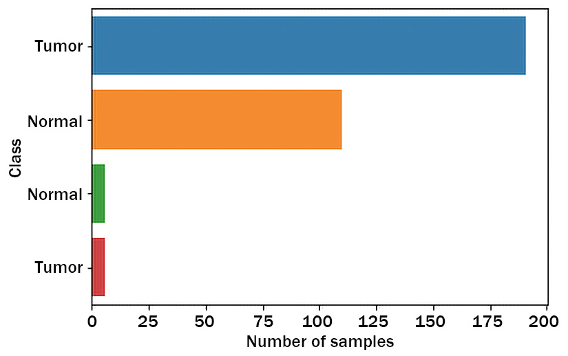
Figure 3.5 – Plotting of lung cancer classes and their values in a bar plot

This bar plot in Figure 3.5 shows how many samples fall into each of Normal and Tumor (lung cancer) types. Oh, no. We have a problem now. As you can see, there are two types of samples, both of which are classified as Normal and the same for Tumor. What be the reason?

3. Let’s look at the different classes closely and see what’s going on:

   set(lung_1_4['class'])

   {' Normal', ' Tumor', 'Normal', 'Tumor'}

Do you see anything weird here? If you look closely, we notice that there is an extra space in front of the first and second classes, because of which we get two extra classes, even though the total number of classes should be only two. This is quite common for public datasets, and this is where EDA will come in handy. Fortunately, this is an easy fix.

4. Let’s rename those right away using the following replace method:

   lung_1_4['class'] = lung_1_4['class'].replace(' Normal', 'Normal')

   lung_1_4['class'] = lung_1_4['class'].replace(' Tumor', 'Tumor')

5. Now that we have fixed the issue, let’s replot using the same code as before and see the class distribution:

Figure 3.6 – Plotting of lung cancer classes and their values in a bar plot after fixing the labels

Now, the plot looks much better and is kind of expected. There are some differences in the number of samples that belong to the Normal class (197) compared to the Tumor class (116), which is expected. This class imbalance will create problems during model predictions, but there are advanced techniques available for addressing class imbalance. However, it is beyond the scope of this tutorial to discuss those techniques.

Data transformation

The next step after data preprocessing and EDA is data transformation. This is an important step because many times, each variable/feature has a different magnitude. So, it is a good practice to scale the data that might come from how the experiments are performed and the potential problems that might occur during data collection. Any systematic differences between samples must be corrected before proceeding to the next step. In this step, we will check if there are such differences using box plots.

Here are the steps:

1. First, we will restrict our dataset to the first 10 columns since it is challenging to visualize all the columns at once in a single boxplot. Then, we convert the data from wide format to long format using the melt method in Pandas:

   lung_1_4_m = pd.melt(lung_1_4.iloc[:,1:12], id_vars = "class")

2. Next, we will use the Seaborn visualization library to look at the distribution of expression across selected samples:

   ax = sns.boxplot(x = "variable" , y = "value", data = lung_1_4_m, hue = "class")

   ax.set_xticklabels(ax.get_xticklabels(), rotation=90)

   plt.xlabel("Genes")

   plt.ylabel("Expression")

Now, let’s visualize the boxplot:

Figure 3.7 – Boxplot showing the gene expression value distribution for 10 samples

As shown in Figure 3.7, each sample has a somewhat similar distribution of gene expression values except for the first few samples (compare the medians). In addition, the expression values are already normalized and there is no need to normalize this further. So, let’s proceed without normalizing these samples.

Data splitting

Once the data is transformed and scaled we are now ready to train the model, but before that, we must split the data into train and test datasets. The reason for splitting into train and test is to have a training set for training the model and keep an independent dataset (test set) for model evaluation.

Note

For this simple exercise, we will not split it into three different datasets (train, validate, and test).

For this purpose, we will use Scikit-learn’s train_test_split function, which can split the data into train and test based on the split ratio. In this case, we will split the train and test datasets in the ratio of 75:25 because we want to use more data for training than for testing, but in the real world, we will have ratios something like 60:40 training : testing.

Data splitting is a multi-step process, so let’s understand this in detail next:

1. Drop the ID and class columns in the dataset, and convert it to a NumPy ndarray, a multidimensional container of items of the same type and size:

   x_data = lung_1_4.drop(['class', 'ID'], axis = 1).values

Similarly, we will create a NumPy ndarray for the labels from the subset data:

y_data = lung_1_4['class'].values

2. Next, we must first convert the categorical data in the type column to numbers. Ordinal encoding and one-hot encoding are the two most popular techniques to convert categorical data to numbers. In this simple tutorial, we will use the ordinal encoding method. Let’s create a variable class to create a unique list of the different classes in the target:

   classes = lung_1_4['class'].unique().tolist()

   classes

   ['Normal', 'Tumor']

3. Next, convert the classes into ordinals using a custom function:

   import numpy as np

   func = lambda x: classes.index(x)

   y_data = np.asarray([func(i) for i in y_data], dtype = "float32")

Printing the y_data array (not shown here) shows the different classes converted to ordinals first and then to floats. Here, 0 represents the Normal class, while 1 represents the Tumor class.

4. Now, we are ready to split the data into training and testing. For this, we will use Scikit-learn’s train_test_split function:

   from sklearn.linear_model import LogisticRegression

   from sklearn.model_selection import train_test_split

   X_train, X_test, y_train, y_test = train_test_split(x_data, y_data, random_state = 42, test_size=0.25, stratify = y_data)

   X_train.shape, X_test.shape, y_train.shape, y_test.shape

   ((234, 58735), (79, 58735), (234,), (79,))

The train_test_split function takes multiple arguments to split the features and labels into four different outputs. For this example, we are specifying a train : test split ratio of 75:25, and also, we are making sure that we will stratify (to make sure that the ratios of all the classes - Normal and Tumor are maintained equally between train and test datasets) the data first before splitting.

Model training

Finally, the exciting part of the exercise is training the model using the training set that we split in the previous step. For this simple exercise, we will use logistic regression. Logistic regression by default classifies data into two categories, which is exactly what we want here. Let us run the Logistic regression with our training dataset. Again, we will use scikit-learn’s linear model method for running Logistic regression on the training data:

model_lung1 = LogisticRegression()
model_lung1.fit(X_train, y_train)

Here, we are first instantiating an object using the LogisticRegression function and using that to fit the training data consisting of features and labels.

Model evaluation

Now that model has been trained, let’s run the model on one sample of the test data. Running the following command outputs the label as part of the prediction:

pred = model_lung1.predict(X_test[12].reshape(1,-1))
pred
array(['Tumor'], dtype=object)

Here, we are using the trained model (model_lung) to predict on one of the samples in the test data (12). The prediction returns a normal sample. As a manual validation, you can check and see if the prediction here matches the actual label in the test data. You can also do predictions for all samples in the test data:

all_pred_lung= model_lung1predict(X_test)

The output here (not shown) indicates the predicted classes for each of the samples in the test data. Now, you can check to see if the class that is predicted by this algorithm is the same as the original class or not.

So far, we looked at model prediction on a single sample, but can we trust the model just based on a single prediction? We will have to check the model predictions on all the test data and compare them with the original labels in y_test data. To assess the performance of our model, we must first define some metrics. There are several metrics that we can use, and it’s beyond the scope of this chapter to go over all of them. We will use two popular evaluation metrics here:

1. The first is accuracy_score, which calculates the accuracy of the model. Accuracy is defined as the number of true positives and true negatives divided by all predictions. Have a look at the following code snippet:

   model_lung1score(X_test, y_test)

   0.9620253164556962

As can be seen from the output, the model has a very score of 96% without doing any optimization (such as cross-validation, model selection, hyperparameter tuning, and so on). This is not bad for this dataset.

2. Let’s run a confusion matrix to indicate how well the model did in terms of true positives, true negatives, false positives, and false negatives:

   from sklearn.metrics import confusion_matrix , ConfusionMatrixDisplay, classification_report

   cm = confusion_matrix(y_test, all_pred_lung)

   disp = ConfusionMatrixDisplay(confusion_matrix=cm, display_labels = ["Normal", 'Tumor'])

   disp.plot()

   plt.show()

Let’s look at the following screenshot as the confusion matrix of the Logistic regression model:

Figure 3.8 – Confusion matrix of the Logistic regression model

Overall, the model did really well classifying the samples correctly for Normal and Tumor. There are a few instances where the model misclassified the samples. For example, there is one sample that the model predicted as Tumor but that is actually Normal (false positives), and there are three samples that the model predicted as Normal but are Tumor samples (false negatives). Please note that the cost of misclassifying a sample is high for false negative samples compared to false positive ones because we don’t want to miss any patient that has a tumor.

3. The second popular metric is classification_report. Let’s use classification_report from Scikit-learn to print classification metrics for our model:

   classification_report(y_test, all_pred_lung)

Let’s look at the following results of the classification report of the lung cancer samples:

Figure 3.9 – Classification report of the lung cancer samples

The most important component of the classification_report metric for classification models is the F1 score, which is the harmonic mean of precision and recall. Here, the F1 score is very good and is close to 1 for all the classes, which indicates that the model has done a good job of predicting the correct class of the sample.

ML challenges in genomics

ML is the backbone of the large-scale analysis of genomic data. ML algorithms can be used to mine biological insights from genomics big data and discover predictable patterns that may be hard to extract by experts. However, there are a few challenges the current ML algorithms face in the analysis of genomic data:

• Although the amount of data coming out of biological systems and genome sequencing is huge and ever-growing, integrating these diverse datasets from multiple sources, platforms, and technologies into ML algorithms is not trivial.
• Because of this huge variation in trained data, models tend to overfit and they generalize very poorly on new data that is different from the training data. We can use methods such as L1 and L2 regularization to address this poor generalization, which we will see in future chapters.
• The nature of ML models, which are mostly “black boxes”, may bring new challenges to biological applications in particular models to predict diseases. Despite several ML interpretability tools, it is hard to interpret the model predictions, especially from a biological point of view, restricting their application in genomics and other biological domains.
• An ML model needs hand-crafted features, which require domain knowledge in biology and genomics. This is a significant problem for non-experts in genomics.

These are a few of the ML challenges in genomics, and in the next chapter, we will look at sophisticated techniques such as deep learning (DL), which can address some of these challenges in genomics. Before we end this chapter, let’s briefly summarize what we have learned so far in this chapter.

Summary

This chapter started with what ML is and how ML algorithms can help genomic applications through their inherent nature of uncovering hidden patterns in the dataset, automating human tasks, and making predictions on unseen data. We looked at the several types of ML algorithms—namely, supervised and unsupervised methods—and understood the main steps in ML methods. Then, we understood the ML workflow for genomic applications.

In the second half of the chapter, we spent quite a bit of time understanding the different steps in ML and what is involved in each step of the workflow. We also introduced the most popular Python packages Pandas and scikit-learn to work on the ML workflow. Finally, we worked on a real-world application of ML on a genomic dataset for identifying the disease state of cancer patients.

This chapter and the preceding chapters are meant for a quick primer on ML for genomics, and with this knowledge and understanding of fundamentals, in the next chapter onward, we will dive into DL for genomics and understand the different algorithms for analyzing large and complex genomic datasets for unraveling meaningful biological insights.