5

Introducing Convolutional Neural Networks for Genomics

In recent years, deep learning (DL) has emerged as a prominent technology in solving complex problems in various domains. Among DL algorithms, convolutional neural networks (CNNs) dominate the current DL applications because of their incredible accuracy in computer vision (CV) and natural language processing (NLP) tasks. A CNN is a type of neural network (NN) architecture that is used for unstructured data and was originally designed to fully automate the classification of handcrafted characters. Some popular applications of CNNs include facial recognition, object detection, self-driving cars, auto-translation, handwritten character recognition, X-ray image analysis, cancer detection, biometric authentication, and so on. Compared to feed-forward NNs (FNNs), which we learned about in the previous chapter, CNNs process multiple arrays using convolutions within a local field, like perceiving images by eye. Thanks to next-generation hardware such as Graphics Processing Units (GPUs) and Tensor Processing Units (TPUs), the current CNN models can be built rapidly and cheaply. In addition, the introduction of DL libraries and frameworks such as TensorFlow, Keras, and PyTorch has enabled the models to be built and learned easily.

In genomics, machine learning (ML) methods have been widely used for solving some complex challenges, as seen in Part 1 of this book. With the availability of massive amounts of data generated from high-throughput sequencing technologies such as next-generation sequencing (NGS), it was evident that it is beyond the reach of state-of-the-art technologies such as bioinformatics and ML to process this data automatically and provide knowledge on prediction-based analysis and biological insights. To address this, various CNN architectures were developed to process non-image data such as DNA sequence data for various applications such as cancer detection, predicting phenotypes from genotypes, gene expression prediction, identifying DNA- and RNA-binding motifs, predicting enhancers, and so on. The goal of this chapter is to introduce you to CNN architectures and applications as they relate to genomics. By the end of this chapter, you will have a good understanding of what CNNs are, different CNN architectures, why they are important in DL, and what some of the popular applications of CNNs in genomics are.

As such, here are the topics that will be covered in this chapter:

• Introduction to CNNs
• CNNs for genomics
• Applications of CNNs in genomics

Introduction to CNNs

Just to refresh your memory, FNNs are fully interconnected NNs where all nodes in the preceding layer are connected to every other node neuron in the next subsequent layer, and so on (Figure 5.1). Each edge or connection has a weight, that is either initialized randomly or derived from domain knowledge and ultimately learned by the algorithm during model training. The weights are then multiplied by the input values from all the node’s neurons, and then the sum of all the nodes in the input layers is then passed on to the next layer, along with a bias that is then used by an activation function to signal whether that output will be passed on to the next layer or not. The process repeats in each layer until the final output layer, which has one to many neurons, depending on the type of learning and whether generating a prediction or classification. FNNs work great for structured data where you have features and samples as input:

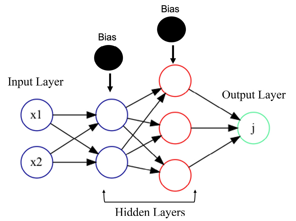
Figure 5.1 – Typical architecture of an FNN

However, using FNNs for unstructured data such as images, audio, text, sequence, and so on would be very challenging. Let’s understand this through an example.

Say our input is a 32-pixel by 32-pixel grayscale image where every pixel in the grayscale image is represented by a value between 0 to 255. Here, 0 indicates black, 255 represents indicates white, and any values between 0 and 255 indicate various shades of gray. Since the grayscale image has only one channel, the image can be represented as 32 x 32 x 1 = 1024, and consequently has 1,024 nodes in the input layer of the FNN. Suppose our next layer (hidden layer) has 100 nodes, and since this should be fully connected to the previous layer, we will have 1,024 x 100 = 102,400 weights for the first 2 layers (input and the first hidden layer). Since we know by now that a complex problem such as this requires multiple hidden layers in the FNN to map the inputs and the outputs in the training data to generate an accurate model, as such, we now have a problem with too many parameters in the FNN, which makes the training process very complex because of the increased dimension space. In addition, it makes the learning process slower, uses more resources, and increases the chances of overfitting.

If we are to use the color images, the problem is further compounded because the color images have 3 channels (red, green, and blue) where each color is represented by a channel, and so in total there are 3 values and 32 x 32 x 3 = 3,072 values. Correspondingly, the number of weights for such an image is 3,072 x 100 = 3,072,000. FNNs cannot scale to handle these kinds of images, so there needs to be a better scalable architecture. Another limitation of FNNs with image data is that the 2D image is converted to a 1D flattened vector, and so the spatial relationship of the different pixels is completely lost. So, there needs to be a better NN architecture that can keep spatial relationships and process unstructured data.

What are CNNs?

CNNs are a special type of NN architecture that is widely applied for unstructured data such as images, audio, video, text, and so on. CNNs are great networks for analyzing data with spatial dependencies such as images, audio, DNA sequences, and so on. They work well on DNA sequence data. The main applications of CNNs include image classification, NLP, signal processing, and speech recognition. CNNs have a series of convolutional layers, which allows them to automatically extract hierarchical patterns in the data. CNNs are currently being used in genomics tasks where local patterns are very important to the outcome—for example, the detection of conserved motifs to identify blocks of genes in a DNA sequence or binding sites of a protein such as a transcription factor (TF). Let’s dive deep into the wonderful world of CNNs in the following sections.

Birth of CNNs

The first idea of a CNN came from Hubel and Wiesel when they reported in 1959 a marked change in neuron activity when a bright light was passed at a particular angle and a particular location to a cat (https://www.ncbi.nlm.nih.gov/pmc/articles/PMC1363130/). It was shown that complex neurons receive inputs from multiple simple neurons in a hierarchical manner. For these findings, they were awarded the Nobel prize in 1981. This report inspired Fukushima, who then developed the first CNN architecture termed Neocognitron to recognize handwritten Japanese characters (https://www.rctn.org/bruno/public/papers/Fukushima1980.pdf). CNNs have a long history, which primarily started with LeCun, who is widely credited for his contribution to advancing CNNs (https://www.persee.fr/doc/intel_0769-4113_1987_num_2_1_1804). However, the breakthrough for CNNs came when a CNN did extraordinarily well against other models at the ImageNet Large Scale Visual Recognition Challenge (ILSVRC) competition.

So, what is a CNN, how does it work, and why is it powerful for unstructured data? Let’s start with understanding CNN architecture.

CNN architecture

Unlike an FNN, the architecture of a CNN is slightly complicated. It consists of an input layer for feeding in the inputs, a convolution layer for performing convolutions, a pooling layer for downsampling the data, a fully connected layer (which is similar to an FNN), and finally, an output layer for making predictions (Figure 5.2). Let's discuss each of these in detail in the following section:

Input layer

As with any NN, the input layer represents the first layer of a CNN. A typical example of an input layer can be a grayscale image, or, in the case of genomic data, it is the sequence of DNA from a patient sample or an experimental sample. Unlike vanilla NNs, there is no need to flatten the input to a one-dimensional vector. Instead, we can provide the images or a DNA sequence directly to the network, which will help to preserve the spatial relationships better.

Convolutional layer

This is the most important layer of a CNN because this is what distinguishes a CNN from an FNN and other architectures. The main feature of CNN is it's use of convolution operations which replace the matrix multiplications in a typical FNN and it's ability to capture spatial information in the data (Figure 5.2). Let’s understand how a convolutional layer works in a typical CNN:

• A convolutional layer consists of multiple filters (also called kernels) that are nothing but the matrix of weights—for example, a filter of size 9 (3 by 3) that is initialized with values randomly between 0 to 10.
• Next, convolution is done by placing this filter at the top-left corner in the case of the image and taking the dot product of the filter values and the input values of the pixel (remember—pixel values range from 0 to 255, but they are normalized to keep the values between 0 to 1) to calculate a feature map, and we will take a step size (stride) of n=1 to the right.
• The process is repeated until we reach the top-right corner of the image, and then we start over again from one down cell from the left of the image until we finish scanning the whole image.
• While convolving the filter, we calculate the dot product of the weights on the filter with the input values. For example, as shown in Figure 5.2, the input size of 5 by 5 (25 in total) is being scanned by a filter of size 9 (3 by 3), and the dot product of the filter values and the input values of the pixel is being calculated in the output array:

Figure 5.2 – Illustration of a convolutional filter along with the input image

In the case of a DNA sequence as an input, after creating a one-hot encoding (Figure 5.3), the convolutions are performed similar to image data. Each filter chosen will act as a sliding window.

Figure 5.3 – Illustration of a convolutional filter along with the input image

Generally, multiple convolutional layers are present in a typical CNN architecture. The first few convolutional layers extract general features from their input data, and the subsequent layers extract more complex features. A non linear activation function such as ReLu or LeakyReLu will be applied to the linear combination of weights in the filter and input values.

Pooling layer

The next layer after the convolution layer is the pooling layer, which reduces the number of parameters, memory usage, and computational cost, and prevents overfitting in the network progressively (Figure 5.4). It is quite normal to have pooling layers between multiple convolutional layers. The pooling layer operates as a downsampling layer, and while doing so, computes either an average or a maximum value for a specified filter size and stride (slide is nothing but a sliding window size):

Figure 5.4 – Pooling layer schematic

For example, as shown in Figure 5.4, the max pooling takes the maximum value (74) from the window, which are 41, 24, 32, and 20, and the average pooling takes the average of all the values from the window, which are 74, 60, 65, and 11. There are no parameters need to be learned from the pooling layer.

Fully connected layer

The last layer before the output layer is the fully connected layer, and this generally lies between the pooling layer and the output layer. Please note that the output from the pooling layer gets flattened before feeding it to the full connected layer. All the nodes from the pooling layer are connected to the fully connected layer to generate the probability of predictions or classifications (Figure 5.5):

Figure 5.5 – Fully connected layer connecting to the output layer

The fully connected layer is the key since it takes the flattened values from the preceding convolutions and pooling layers, then behaves as a mini FNN, and then connects it to the output layer (Figure 5.5).

Output layer

This is like any other output layer as we have seen in a typical FNN. The output layer uses a function such as Softmax or Sigmoid to predict or classify the output depending on the problem.

So far, you have been looking at individual components of a CNN one at a time. Let’s now visualize a full CNN end-to-end (Figure 5.6). As indicated previously, a typical CNN usually consists of multiple convolutional and pooling layers. The convolutional layers along with the pooling layers are very important as they are responsible for feature extraction, which is a powerful feature of a CNN, unlike other architectures. In this example, the input such as an image (here, the image representing 0) or a DNA sequence in the form of a one-hot encoding matrix is fed into the CNN model, which goes through several convolutional, pooling, flattening, fully connected and finally, gets predicted in an output layer:

Figure 5.6 – A typical CNN with convolution layers

Now that we have understood what a typical CNN architecture looks like, let’s take a small detour and learn about transfer learning (TL), which is a powerful concept in CNNs and other NNs.

Transfer Learning

Transfer learning (TL) is where we leverage a pre-built model on a new task. In other words, a model that was trained on a particular task is reused on a different but related task to repurpose the existing model without building a completely new model from scratch. In TL, the learned feature from the pre-trained model is transferred to facilitate the prediction or classification of untrained datasets. It’s like taking a model and using it for prediction purposes without training the model from scratch (Figure 5.7). Through the process of TL, we can achieve significantly higher accuracy compared to training a model from scratch with only a limited amount of trained data and labels:

Figure 5.7 – How TL helps in CNN tasks

As shown in the preceding diagram, a CNN model is typically trained on datasets that are large so that the model can learn the features effectively compared to smaller datasets. Once this model is trained on this big data, then it can be used to retrain with smaller data specific to a particular problem, and then the model can not only be trained effectively but also produce highly accurate results.

TL is quite common in DL, especially for applications such as CV and NLP-related tasks where it is not always possible to get a large amount of data along with the target labels for model training. It is rare for researchers and scientists to build models from scratch; instead, they prefer to start from a pre-built model that has already been built for doing a similar task—for example, model that can classify different sequences and has learned general patterns of the data. The same can be said for genomics. Many times, it is not possible to build a model for genomics problems due to the absence of labeled data, smaller-sized samples compared to the number of genes, and so on. In this instance, the TL method can aid the genomics field by incorporating the complex features learned by the model on the trained data and using that to predict or classify the novel data. A few examples include predicting cancer types, identifying potential biomarkers for small or large untrained datasets, predicting gene expression, and so on.

CNNs for genomics

Even though CNNs are primarily used for unstructured data such as images, text, audio, and so on, they are also powerful tools for non-image data such as DNA. Unfortunately, the raw DNA sequence data cannot be provided to CNNs as input for feature extraction. It has to be converted to numerical representation before it can be used by CNN. The first thing to note for non-numeric data such as a DNA sequence is that you will have to first convert the 1D DNA sequence data to a one-hot encoded structure (Figure 5.8):

Figure 5.8 – Example of one-hot encoding for a DNA sequence

As shown in the preceding diagram, each nucleotide in the DNA sequences is represented as a one-hot vector: A = [1000], C = [0100], G = [0001], and T = [0010]. The one-hot encoded matrix can then be fed into the model for training purposes. Please note that one-hot encoding is not the only way of representing DNA sequences to a CNN. There is also label encoding in which each nucleotide (A,G,C,T) is represented by a unique index thereby preserving the positional information. For example A=1, G=2, C=3, and T=4. Let’s try to understand why a CNN architecture is great for genomics problems using cancer prediction from Single nucleotide polymorphisms (SNP) variants from multiple patient samples as an example.

In the case of using FNN for cancer prediction, the first layer receives the SNP variants as input, and the weighted sum of each input value plus the “bias” (constant) is then passed through a non-linear function such as ReLu. This process repeats in the subsequent hidden layers until it reaches the output layer where it is transformed via sigmoid or softmax activation function to produce the hidden neurons output value. Although FNNs are powerful for this example, they are certainly not suitable for spatial or temporal datasets, and in genomics, there are several problems that are either spatial or temporal, and predicting cancer from SNPs is one of them. CNNs can address these issues. In the case of cancer prediction from the SNP data problem, SNPs are distributed according to a particular space pattern. So, a convolutional operation with predefined width and strides is performed on the input data. In this example (Figure 5.9), the convolutional operation is done using a kernel size of 1 by 3 and with a stride of 1. After multiple convolutions in one or more convolutional layers, the next layer is the max pooling layer, which takes the maximum of all values for each of those positions from kernel outputs using a predefined filter size. Pooling layers are then flattened and connected to a non-linear fully connected layer and finally to an output layer that has a binary class (cancer or no cancer) (Figure 5.9):

Figure 5.9 – Simple schematic of a 1D convolutional operation for SNP data

As you can see in the preceding diagram, CNNs are thus very powerful for spatial interactions and are translation-invariant, and so are routinely used in genomic applications where both spatial and temporal interactions are quite common. In the next section, we will learn some of the most popular applications of CNNs in genomics.

Note:

We will see an use case of of how to build CNNs for predicting the binding site location of a Transcription Factor (JUND) in Chapter 9, Building and Tuning Deep Learning Models. For now, let's look at the different applications of CNNs in genomics in the next section.

Applications of CNNs in genomics

Now that you understand how CNNs work in genomics with a simple example, let’s look at some of their applications that are popular in genomics.

DeepBind

TFs are DNA- and RNA binding proteins that play a crucial role in gene regulation. Knowing the binding sites of these DNA- and RNA-binding proteins would help us to develop models and can help identify disease-causing variants. One way to infer the sequence specificities of these proteins is through position weight matrices (PWMs), which can be used to scan the entire genome to identify potential binding sites of these DNA- and RNA-binding proteins. In addition, DNA- and RNA-binding protein specificities are measured by several high-throughput assays such as PBM, SELEX, and the most popular ChIP- and CLIP-seq techniques. Some of the challenges associated with this data are that the raw data comes in several different quantitative forms, the data is often extremely huge, and each data generation methodology suffers from artifacts, biases, and limitations that hinder the identification of binding sites. DL techniques show more promise in capturing sequence specificities of these binding proteins. DeepBind (https://pubmed.ncbi.nlm.nih.gov/26213851/) is a CNN architecture that was built to predict DNA- and RNA-binding protein binding sites in the genome. It takes in noisy experimental data and outputs a binding affinity of a DNA- or RNA-binding protein to indicate how likely it is that the TF will bind to the sequence.

DeepBind takes in a set of raw sequences with lengths ranging from 14 to 101 base pairs, along with an experimentally determined binding value as a label or target. From this data, it calculates the binding score in four stages—the convolutional stage, which scans the sequences with a set of motif detectors (4xm matrices) such as PWMs. The next is the rectification stage, which isolates any patterns by shifting responses of the motif detector and clamping any negative values to 0 using the ReLu activation function (remember—ReLu takes in a value and gives either 0 or the maximum of the value, whichever is the greatest). Following the rectification is the pooling stage, where the model calculates both the average and maximum value for each motif detector. The max pooling will help the model get the longer motifs or patterns, whereas the average pooling will help the model pick up the combined effect of shorter motifs.

The pooled values are then flattened and fed into the fully connected layer (non-linear NN) to produce the scores. The rest of the steps are typical of any FNN, which is to use backpropagation, cross-validation, and so on to optimize the weights and improve the model accuracy. The optimized DeepBind model is evaluated on test data to predict binding affinities and model performance using metrics such as AUC. Using DeepBind, you can now simply change the nucleotide position of a protein of interest and see how that affects the binding affinity of a TF in terms of positive or negative binding. Since DeepBind can find relationships between mutations and the dishes that cannot be inferred from traditional methods, researchers have used DeepBind to see where certain mutations in the cholesterol gene can disrupt the binding affinity of a TF.

DeepInsight

DeepInsight (https://www.nature.com/articles/s41598-019-47765-6) is a CNN model that was built to extract features from genomics data. The idea of DeepInsight is simple. It takes non-image data such as genomics, transforms it into image data, and then feeds it into a CNN for classification or prediction depending on the problem. Instead of feature extraction and selection for collected samples ( samples x features), DeepInsight finds a way of arranging closely related features into neighboring regions ( features x samples), and all dissimilar features are kept further apart with the goal of learning complex relationships and interactions. Arranging similar elements together is a powerful method for uncovering hidden mechanisms such as pathways in biological systems. This approach of clustering similar features is more powerful than handling each feature separately, which ignores the neighborhood information that is key for spatial and temporal datasets. With this simple idea, it can transform any non-image data into feature map images, which can be a friendly representation of samples to a CNN architecture.

DeepChrome

Among several factors that control transcriptional regulation, histone modification is the primary factor. Histone nucleosome proteins and histone modification through methylation is a very common gene regulatory mechanism. Understanding of the combinatorial effects of histone modification and gene regulation can help in developing epigenetic drugs for cancer. Researchers are interested in inferring the gene expression from methylated data, and so multiple computational models, both rule-based, which try to capture the relationships between histone modification and gene expression, and ML models such as linear regression, support vector machines (SVM), and Random Forest, have been proposed for gene expression predictions based on histone modification. However, neither of these methods have been successful. DeepChrome (https://academic.oup.com/bioinformatics/article/32/17/i639/2450757) is a CNN-based architecture that was designed to capture the interactions among histone modifications and use that to predict gene expression. If you recall, we have seen an example of methylation prediction using manually extracted features in Chapter 4, Deep Learning for Genomics. DeepChrome, allows automatic extraction off complex interactions or most important features without us manually extracting the same as we have done before.

DeepVariant

NGS technologies have allowed scientists and clinicians to produce sequencing data rapidly, cheaply, and at scale and apply it broadly to fields such as health, agriculture, and ecology. Accurate detection of genetic variants (SNPs and indels) from sequencing data is important for scientists and clinicians for disease detection, identifying genetic disorders, and making discoveries. DNA sequencing of genomes to identify genetic variants involves two key steps:

1. Sequencing of the samples, which generates relatively short pieces of DNA (reads)
2. A variant caller that maps the reads against the known reference to identify where and how a sample’s genome sequence is different from a reference genome

The current variant callers often struggle to accurately identify the correct variants and, in the process, generate lots of false-positive and false-negative variants. Accuracy of the variant detection is important because a false-negative variant indicates missing the causal variant for a disorder while the opposite (a false positive) means identifying the wrong variant. DeepVariant (https://www.nature.com/articles/nbt.4235) is a CNN-based framework that converts variant identification problems into image classification problems. It takes the input data, which is aligned sequences (reads) to the reference, and constructs multichannel images representing some aspect of the sequence—for example, one channel can be read base, the second channel is the mapping quality, and the third channel is read supports allele, and so on. Finally, DeepVariant generates one of three genotype likelihoods (0, 1, or 2) of given alternate alleles in each sample. Using this unique design, DeepVariant outperformed state-of-the-art variant detection tools. The model can be used across other genomes allowing nonhuman sequencing projects to benefit other genome projects. In addition, DeepVariant can be leveraged for other sequencing technologies and experimental designs highlighting the importance of this architecture.

CNNC

A CNN for coexpression (CNNC) (https://www.biorxiv.org/content/10.1101/365007v2) is a supervised CNN architecture that uses gene expression data to understand relationships between genes. Each pair of genes is represented as a histogram, and a CNN model is trained with training examples that have both positive and negative samples. Some examples of these include known targets of a TF, known pathways for a specific biological process, known disease genes, and so on. First, the gene expression levels from each pair of genes are transformed into 32 x 32 normalized empirical probability distribution function (NEPDF) matrices. Next, each NEPDF matrix is fed into the network as an input. The other input types can be DNase-Seq, PWM data, and so on. After going through the convolutions, finally, the output of a CNNC can either be a binary classification or a multi-class classification.

Summary

DL has made massive strides in several domains of life sciences and biotechnology, including genomics. CNN architecture is mainly designed for unstructured data. It accepts the input image or a DNA sequence (matrix of size x ) as an input, extracts the features from the image, and does the prediction or classification through a series of hidden layers such as a convolutional layer, a pooling layer, a non-linear fully connected layer, and an output layer. CNNs do not require any separate feature extraction step and automatically derive features from the input data. CNNs have revolutionized the field of genomics because of their incredible accuracy and ability to process unstructured data, which is quite common in genomics.

In this chapter, we have looked at the history of CNNs, what they are, and the different components of CNN architecture. Later in the chapter, we understood how CNNs are being leveraged in genomics for studying complex problems such as gene expression, gene regulation, genetic variant detection, and so on. In the final section of the chapter, we have seen different CNN architectures for solving genomic problems. Hopefully, this chapter gave you a taste of CNNs and what they can do to solve some of the complex challenges in genomics. In the next chapter, we will learn about another incredible architecture that is even becoming more popular than CNNs for genomics: recurrent NNs (RNNs).