10

Model Interpretability in Genomics

Deep learning (DL) methods have been widely adopted in genomics for extracting biological insights and model predictions because of their superior performance in predictions and classification tasks through their deep neural network (DNN) architecture. Even though the accuracy and efficiency of these model predictions are the primary goals of DL in genomics applications, the decisions made by these DNNs is also important in genomics toward the goal of understanding cellular and molecular mechanisms. In Machine Learning (ML) and DL, "Model interpretability" refers to how easy it is for humans to understand the decisions made by the model. The more interpretable the models are, the easier is it to understand the model's decisions. In contrast, difficulties in model interpretation limit the practical utility of DL models and reduce confidence in their adoption. However, it’s not easy to interpret DL model behavior in a way that humans can understand because of the features they use to draw conclusions and the mathematical calculations they use and hence they are referred to as black-box models. It is important to understand why a model has made decisions before it is put into production, especially in domains such as life sciences, biotechnology, genomics, medicine, healthcare and so on.

Model interpretability is one of the hottest areas of DL research and is a complicated subject. By interpreting the model’s behavior, we can fill in the gaps in our understanding of how models work and increase the trust in the models that are built using DL. Model interpretability can be used to discover the knowledge of the model, justify the model predictions, and improve the model. In addition, model interpretability is often a key factor when a model is used in the product, a decision process, or research. However, model interpretability is not easy to perform, especially with DL models, where it is even harder because of the complexity of the model, leaving few clues for researchers about the underlying behavior of these models. Thankfully, several model interpretability methods and tools exist that can help researchers to help interpret model behavior. In this chapter, you will be introduced to gentle concepts in DL model interpretability. Model interpretability introduced here helps genomic researchers and other scientists to understand the business context of building models and using the same for predictions. By the end of the chapter, you will have learned what model interpretability is and an introduction to the tools for performing model interpretability to uncover biological insights from genomic datasets. As such, here is the list of contents that will be covered throughout the rest of the chapter:

• What is model interpretability?
• Unlocking business value from model interpretability
• Model interpretability methods in genomics
• Use case – Model interpretability for genomics

What is model interpretability?

Deep learning's popularity is mainly because of the sophisticated algorithms such as DNNs it uses to perform complex tasks. If trained popularly, the models are not only accurate but also generalize very well on real-world data. DL, with its ability to extract novel insights using automatic feature extraction and to identify complex relationships in massive datasets showed superior performance compared to the state-of-the-art conventional methods. The promise of these DL models, however, comes with some limitations. With their black-box kind of nature, these DL models face problems in explaining the relationship between inputs and predicted outputs or, in other words, model interpretability. It is humanly impossible to follow the reasoning for a particular prediction using these black-box models. You might be wondering if the DL models perform and generalize well, why you would not trust the model that it is making the right decisions. There can be two possible reasons:

1. Firstly, as we saw in Chapter 9, Building and Tuning Deep Learning Models, model evaluations are mainly done using few model metrics, which is an insufficient to evaluate how models work on real-world tasks.
2. Secondly, because these DL models are currently being used for high-stakes decision-making in many domains including healthcare, medicine, pharmaceuticals, and so on, there must be much clarity on how these predictions or why a particular decision is made by the model to build trust.

There is a lack of understanding of these concepts compared to how data is entered and how final choices are made. No matter how accurate these models are and how advanced our understanding of biological mechanisms is, how can we trust these models if we don’t understand how they work?

Black-box model interpretability

Before we discuss model interpretability as it relates to DNNs, let’s first understand the concept. Most machine learning (ML) models are interpretable, which means it’s easy for humans to understand why the model made those predictions. For example, the simplest ML model is linear regression, in which the final output prediction is the weighted sum of all the features from the input and the bias term. The easiest way of understanding the linear regression model is to look at the coefficients (weights) that are learned during model training for each feature. These coefficients indicate how much the model output changes when 1 unit of values of input features, whereas, in the case of DNNs, they are generally referred to as “black-box” models because of their complex architectures and hard-to-interpret model decisions. So why is it hard to interpret a DNN model prediction?

Here is an example of a simple fully connected neural network (NN) architecture that you have seen multiple times before (Figure 10.1). Even with this simplest of NN architectures, it’s hard to understand which feature is contributing to the final model output because of several layers and multiple nodes per layer:

Figure 10.1 – A simple two-layered NN

If we cannot explain how the model predictions are made with this simplest of NN architectures, now imagine we have a DNN with millions of neurons and several hundred layers, as shown here:

Figure 10.2 – DNN architecture example

Interpreting a model with this complicated NN architecture as shown above is even more challenging and humanly impossible.

The challenge in model interpretability faced by current DL models applies to the field of genomics as well because several genomic applications rely on DNNs for predictions and classification-related tasks, as seen before. For example, in the previous chapter, we built a DL classification model for transcription factor binding sites (TFBS) predictions. We can now use the model on an unknown DNA sequence to predict if it contains TFBS or not, but we don’t know how and why these predictions are made by the model. This is where model interpretability is helpful. Model interpretability algorithms will not only help with interpreting the model decisions but also augment at several points in the DL life cycle phases such as data collection, model training, and model monitoring, as seen in the following diagram:

Figure 10.3 – How can interpretation methods help in a typical DL life cycle?

At each of the three stages shown in Figure 10.3 (data collection, model training, model deployment), current model interpretability methods can help address the problem of model interpretability.

Unlocking business value from model interpretability

When it comes to predictive modeling, there is a trade-off between wanting to know what is predicted or why a prediction was made, or you do not care why a decision was made. Each of those scenarios depends on the use case. For example, if you are building a model for research and development (R&D) purposes, then you would sacrifice model interpretation over accuracy, whereas if you are building a model for business use, it is important to understand how the model is making that decision. Either way, it is important to know the model’s behavior not only to understand why some decisions were made but also for debugging and model improvement.

Let’s now understand why model interpretability for DL is important and how it helps to unlock practical business benefits such as better business decisions, building trust, and increasing profitability in the following section.

Better business decisions

Before model deployment, the models are evaluated on a test dataset, as seen in Chapter 9, Building and Tuning Deep Learning Models, using one or more evaluation metrics such as accuracy, AUC, and so on. When a company decides to deploy this model as an application to use real-world data, relying on this single metric may lead to new questions such as “Which of the input features are impacting the final model performance and predictions?”, “Can those predictions be trusted with real-world data?”, or “Can I trust my model since it is performing exceptionally well?” and so on. If this model is deployed for non-risky tasks, then the penalty for making a wrong prediction is low, but if the model is deployed for business use cases, focusing on just the evaluation metrics is not enough. We must understand model decisions for reasons such as model improvement, debugging, trust, compliance, and so on.

Let’s understand this through an example.

It is well known that current cutting-edge targeted therapy to treat Cancer, even though works great, suffer from several limitations such as laborious, expensive, time consuming, and so on. DL is a great method to address this limitation and surpass current state-of-the methods in drug response predictions because they capture intricate biological interactions to the specific drug.

For example, if a company is interested in producing a drug to treat cancer and based on their research, they find that “undruggable proteins” such as transcription factors (TFs), which are involved in transcription mechanisms, can be potential targets for cancer drug development or target therapy. They now collect lots of genomic data from several genomic databases such as the Gene Expression Omnibus (GEO), The Cancer Genome Atlas (TGCA), the Cancer Cell Line Encyclopedia (CCLE), pharmacogenomics database and so on. Then, they trained a DNNs.

The following diagram provides a visual representation of such a DNN model:

Figure 10.4 – A simplified illustration of a DNN model for identifying anticancer targets from genomic data

Before they use the trained model to predict patient drug response and then develop anticancer drugs based on those predictions, they have three possible routes:

• They might be interested in knowing the probability of how effective the developed anticancer drug is for the patient
• They care about model interpretability as to why the model made that decision/prediction
• They do not care why a decision was made or if it made the right decision

Among the three scenarios, knowing why made that prediction can help them learn more about the problem, the data, and the reason. If the model is mainly used for R&D and a mistake may not have serious consequences, then you probably don’t care about the model’s decisions. In general, model interpretability can lead to an improvement in the model. Model interpretability can sometimes lead to the identification of outliers which can either lead to potential revenue opportunities or potential liabilities waiting to happen and both help companies help prepare and strategize decisions.

Building trust

For organizations, trust is their reputation and is something that cannot be bought with money. The goal of model interpretability is to make models better at making decisions. If the models fail, at least they should explain why they would have failed. So, having good model interpretability is key for a model to build trust among the company and the stakeholders involved. There is no substitute for that.

Profitability

If model interpretability ensures better decisions, builds trust, and improves model predictions, then this will lead to its increased use and enhance overall brand reputation, and ultimately increased financial revenue. In contrast, if there are concerns with any of those issues, they will adversely impact both profits and reputation.

Model interpretability methods in genomics

The field of genomics has garnered so much attention lately because of the advances in high-throughput methods, such as next-generation sequencing (NGS), and other omics technologies such as proteomics, metabolomics, and so on. This has resulted in abundant data such that researchers are in a dilemma about how to use this. The DNN methods showed superior performance compared to the state-of-the-art conventional methods in many genomics applications in medical research, especially in imaging tasks, tumor identification, antibody discovery, motif finding, genetic variant detection, and chromatin interaction, to name a few. However, the major complaint from DNN architectures is that they are black-box models. What that means is that we don’t know how these models made decision on a given dataset. To make predictions with a DL model, the input data is passed through several layers of a DNN, each layer containing several nodes that have learned weights and activation functions. This is a complicated process that involves millions of mathematical operations, and humans can’t comprehend the exact mapping from input data to prediction. To provide insights into DNN model behavior, researchers have come up with interpretability methods.

Several methods and tools for model interpretability exist for DNNs so that humans can easily understand them. These methods visualize features and concepts learned by the DNN during training, explain individual predictions made by the model, and simplify DNN model behavior. These model interpretability methods can be broadly divided into global and local. Global methods aim to understand how a model decides overall, whereas local methods do it for a single instance. There are several methods currently available for both types, with the goal of model interpretability and improving models. Let’s look at some of the model interpretability methods for DNN now.

Partial dependence plot

In the linear regression model, we have seen how model coefficients or weights can be used to understand model behavior. However, coefficients are not a good way of measuring feature importance to interpret models, mainly because the coefficients rely on the value of the input features. The more realistic measure of feature importance for a model is to understand how changing the feature impacts the output of a model. A partial dependence plot (PDP) is a way to address that (Figure 10.5). A PDP shows how each variable or predictor affects the model predictions. This helps researchers to make sense of what happens when various features are adjusted.

Figure 10.5 – A simple PDP illustrating the feature importance of a simple model

In the preceding diagram, the gray horizontal line shows the expected value of the model when applied to the dataset, while the gray vertical line shows the average value of a particular feature (in this example, the age of the patient). The blue line represents the average model output when we fix a particular feature (in this example, the age of the patient) to a given value. The blue line always passes through the intersection of the two gray lines.

Individual conditional expectation

The individual conditional expectation (ICE) method differs from PDP in that, instead of plotting an aggregate effect of all samples, ICE displays the dependence of the prediction on a feature for each sample separately in the plot (Figure 10.6). This is more useful because it shows the minor variations of all samples when one chose to test on a particular feature of interest.

Figure 10.6 – A simple ICE plot illustrating the feature importance of a simple model

Going by the preceding example, the ICE plot shows the feature importance of a particular feature, but instead of showing the average of all the samples, it shows the dependence of the prediction for each sample separately. Even though ICE gives the more granular level of details about the model predictions and how they related to each sample, it is advisable to try both PDP and ICE for model interpretability

Permuted feature importance

Permuted feature importance (PFI) is a neat method for model interpretability. The idea is simple. For each feature, PFI measures the impact of the shuffling of the feature on the final model prediction error. If the shuffling of the feature increases the model prediction error, then that feature is deemed important, and if not, the feature might be not that useful for the model performance. This is because if that feature is important for the model prediction, a slight change in that feature would affect the model. In contrast, the low-impact feature doesn’t affect the model prediction despite shuffling. Let’s understand this using an example:

Figure 10.7 – An example of how to calculate PFI for one feature

In the preceding diagram, the table on the top left shows the three features from the original table and the predictions made. Then, we shuffle the Thermodynamic stability column, and then the corresponding prediction is calculated. Then, we take the average of the two model predictions to calculate the PFI for the permuted feature (in this case, thermodynamic stability). If the model relies on thermodynamic stability, then the feature importance will be very high, and in contrast, if the model doesn’t rely upon it, then shuffling does not affect the feature importance. We keep repeating the same problem for the rest of the features.

Global surrogate

This is an interpretable model that is trained to approximate the prediction of the full black-box model. First, you take the trained model and make predictions on a test dataset and then train an interpretable model such as a simple ML model such as Random Forest son a prediction made by the black-box model (Figure 10.8). This newly trained interpretable model becomes a surrogate model for the DNN model and now we just need to interpret the surrogate model:

Figure 10.8 – Global surrogate method illustration

However, this method introduces additional error because it uses an interpretable model as a proxy for the black-box model and this method can only predict black-box models but cannot predict the data directly.

LIME

Local Interpretable Model-agnostic Explanations (LIME), as the name suggests, is a local model interpretability method that explains the model behavior for a single instance. Unlike the global method, it cannot explain the whole model. It trains interpretable models such that it approximates individual predictions.

Shapley value

Shapley is one of the most popular model interpretability methods for understanding how the features of the model are related to the outputs. This method comes from coalitional game theory, where each feature is a “player” and the prediction is the “payout”. The idea of Shapley is to use game theory to interpret the model. Shapley values indicate how fairly the payout is distributed among the features (players) and hence are good for interpreting models.

ExSum

ExSum (short for Explanation Summary) is a recent mathematical framework to formally quantify and evaluate the understandability of explanations for models. The main advantage of ExSum compared to other methods is that this method can help provide insights about model behavior not just on a handful of individual explanations that other methods might miss. This method can provide a detailed picture of the entire model’s behavior that we didn’t know previously. ExSum tests a rule across the whole dataset instead of a single instance using three metrics—coverage, validity, and sharpness. The coverage metric indicates how broadly the rule may be applicable over the entire dataset, the validity metric signifies the percentage of specific examples that agree with the rule, and sharpness indicates how accurate the rule is. Simply put, we can use ExSum to see if a particular rule holds up using the aforementioned three metrics. ExSum is very powerful, and if a researcher seeks a deeper understanding of how the model is behaving, they can use it to test specific assumptions.

Saliency map

A saliency map is a frequently used method for measuring the nucleotide importance in a sequence. As a genomic researcher or a data scientist working on genomics data and interested in motifs on a DNA sequence, it is natural to think about which parts of the sequence are most important for the classification of the sequence. For instance, for the model we trained in the Chapter 9, Building and Tuning Deep Learning Models to predict a TFBS, it is important to understand why the model made some decisions that way. Saliency maps are one way of visualizing those patterns. Saliency maps show how the response of an output variable changes with a small change in the inputs (in this case, nucleotide sequence). These saliency maps are extremely useful visualization tools that can help us to understand the binding sites of a particular protein (in this example, TF), as shown in Figure 10.9:

Figure 10.9 – An example of how to visualize scores on individual sequences

The preceding plot shows the ground-truth location of the motifs generated using saliency maps.

Use case – Model interpretability for genomics

In this hands-on exercise section, we will build a similar convolutional NN (CNN) model that we built in Chapter 9, Building and Tuning Deep Learning Models, but unlike in Chapter 9, here we will use a simulated dataset of DNA sequences of length 50 bases (whereas in Chapter 9, we have DNA sequence of length 101 bases). In addition, the binding sites in this example are not just for Transcription Factors (TFs) but any protein. The labels are designated as 0 and 1, corresponding to positive and negative binding sites (0 = no binding site and 1 = binding site).

The goal of this is to train a CNN model to predict the DNA binding site of the protein and visualize it in the predictions. Since these are artificial sequences, we have injected the AAAGAGGAAGTT motif into the positive sequence, but don’t worry—the CNN doesn’t know that.

Data collection

For this hands-on tutorial, we will use the simulated data (code not shown) in which we injected motifs treated as positive sequences and the rest as negative sequences. Follow the next steps:

1. Load all the necessary libraries, shown as follows:

   from keras.layers.convolutional import Conv1D, MaxPooling1D

   from keras.layers.core import Dense, Flatten

   from keras.models import Sequential

   from keras.callbacks import EarlyStopping, ModelCheckpoint

   import numpy as np

   Import pandas as pd

   from sklearn.metrics import roc_curve, auc, average_precision_score

   from sklearn.model_selection import train_test_split

   from sklearn.preprocessing import LabelEncoder, OneHotEncoder

2. Load the sequence data, shown as follows:

   input_fasta_data = pd.read_table("sequences_mod.txt", header=None)

   input_fasta_data.rename(columns={0: "sequence"}, inplace=True)

   sequence_length = len(input_fasta_data.sequence[0])

Let’s move on to the next step.

Feature extraction

The next step will be to convert the sequences to a format that the CNN or any other DL model can accept, which is one-hot encoding. Since we have learned about that already in Chapter 9, Building and Tuning Deep Learning Models and a few other chapters, we will skip the explanation here.

Let’s see how we can leverage the available sklearn package for doing the same:

iec = LabelEncoder()
ohe = OneHotEncoder(categories='auto')
seq_matrix = []
for sequence in input_fasta_data.sequence:
iecd = iec.fit_transform(list(sequence))
iecd = np.array(iecd).reshape(-1, 1)
ohed = ohe.fit_transform(iecd)
seq_matrix.append(ohed.toarray())
seq_matrix = np.stack(seq_matrix)
Print(seq_matrix.shape)
(2000, 50, 4)

Target labels

So, now we have the input features ready, let’s go ahead and collect the labels or targets from the same source:

labels = pd.read_csv('labels.txt')
Y = np.array(labels).reshape(-1)
Print(Y.shape)
(2000,)

Train-test split

Before we train the model, let’s split the dataset into training and test datasets so that we can use training data for model training and test data for model evaluation:

X_train, X_test, Y_train, Y_test = train_test_split(seq_matrix, Y, test_size=0.25, random_state=42, shuffle=True)
X_train.shape, X_test.shape, Y_train.shape, Y_test.shape
print(X_train.shape)
print(Y_train.shape)
(1500, 50, 4)
(1500,)

We’ll now reshape the data so that it corresponds to the input format of Keras:

X_train_reshaped = X_train.reshape((X_train.shape[0], X_train.shape[1], X_train.shape[2], 1))
X_test_reshaped = X_test.reshape((X_test.shape[0], X_test.shape[1], X_test.shape[2], 1))
print(X_train_reshaped.shape)
print(X_test_reshaped.shape)
(1500, 50, 4, 1)
(500, 50, 4, 1)

Creating a CNN architecture

Now that we have the training data ready, let’s build a CNN model and train it first. We will use the DL library Keras.

We will start training with a fairly simple CNN model with a single convolutional layer followed by a single max pooling layer, and then finally, a single dense layer. We also have an output layer consisting of 1 node corresponding to the model predictions (0 or 1):

model = Sequential()
model.add(Conv1D(filters=32, kernel_size=12,
input_shape=(50, 4)))
model.add(MaxPooling1D(pool_size=4))
model.add(Flatten())
model.add(Dense(16, activation='relu'))
model.add(Dense(1, activation='sigmoid'))
model.compile(loss='mean_squared_error', optimizer='adam')

Model training

Now that we have finished compiling the model, we are ready train the model. We feed the model with our training data (features and labels), define a batch size since we are training in the batch model, and set the number of epochs. 10 epochs would give us enough results to evaluate, and we can then ramp up if there is room to improve.

Let’s quickly run it and see how well we did the model training:

callback = [EarlyStopping(monitor='val_loss', patience=2),
ModelCheckpoint(filepath='model_int_genomics.h5', monitor='val_loss', save_best_only=True)]
history = model.fit(X_train_reshaped, Y_train,
batch_size=10, epochs=10,
validation_data=(X_test_reshaped, Y_test))

You will notice two other things here: callback and history. callback is mainly to ensure the model stops once it finds a good stopping point, and then the history variable mainly serves to monitor the loss and accuracy of the training and validation datasets during the training process:

Next, we will plot the training and validation loss to visualize how well we did with respect to model training

plt.plot(history.history['loss'])
plt.plot(history.history['val_loss'])
plt.title('model loss')
plt.ylabel('loss')
plt.xlabel('epoch')
plt.legend(['train', 'validation'])

Let’s visualize the model loss plot:

Figure 10.10 – Model loss plot

The model loss plot shows that even though there are 10 epochs, the model has done really well by keeping the training loss low at lower epochs, and the validation plot also looks great.

Model evaluation

Now that the model is trained, we can evaluate the model against the test data. Do note that the predictions are between 0 and 1 because of the sigmoid activation.

Here’s what we do for calculating model metrics for model evaluation:

• We get the function of the last layer in the NN:

  pred = model.predict(X_test_reshaped, batch_size=32).flatten()

  print("Predictions", pred[0:5])

• We can also calculate the AUC to get an estimate of how well the NN actually learned:

  fpr, tpr, thresholds = roc_curve(Y_test, pred)

  print("AUC", auc(fpr, tpr))

  print("AUPRC", average_precision_score(Y_test, pred))

  16/16 [==============================] - 0s 952us/step

  Predictions [0.9709498 0.00785227 0.97798 0.99865 0.00150004]

  AUC 0.9986542559156667

  AUPRC 0.9985575535116882

Model interpretation

This is what you all have been probably waiting to see how well the model made those decisions. For this, we will generate saliency maps or motif plots, which you have learned about before.

Let’s make a motif plot, as follows:

1. Let’s pick a sample from the test data:

   plot_index = np.random.randint(0, len(X_test), 1)

2. Get the Y ~ X for the chosen sequence that we want to plot:

   seq_matrix_for_plotting = seq_matrix.reshape((seq_matrix.shape[0], seq_matrix.shape[1], seq_matrix.shape[2], 1))[plot_index, :]

   plotting_pred = model.predict(seq_matrix_for_plotting, batch_size=32).flatten()

3. Calculate the gradient—generate a new set of X where for each sequence, every nucleotide is consecutively set to 0:

   tmp = np.repeat(seq_matrix_for_plotting, 50, axis=0)

   a = np.ones((50, 50), int)

   np.fill_diagonal(a, 0)

   b = np.repeat(a.reshape((1,50,50)), seq_matrix_for_plotting.shape[0], axis=0)

   c = np.concatenate(b, axis=0)

   d = np.multiply(tmp, np.repeat(c.reshape((tmp.shape[0], 50, 1, 1)), 4, axis=2))

   # Calculate the prediction for each sequence with one deleted nucleotide

   d_pred = model.predict(d, batch_size=32).flatten()

   # Score: Difference between prediction and d_pred

   scores = np.reshape((np.repeat(plotting_pred, 50) - d_pred), (len(plot_index),50))

4. Make the actual plot:

   import motif_plotter

   import matplotlib.pyplot as plt

   for idx in range(0,len(plot_index)):

   fig=plt.figure(figsize=(18, 5), dpi= 80)

   ax=fig.add_subplot(111)

   motif_plotter.make_single_sequence_spectrum(ax,

   seq_matrix_for_plotting[idx].reshape((50, 4)),

   np.arcsinh(scores[idx]).reshape(50,1))

   plt.show()

Running the preceding command will generate a saliency map, as shown here:

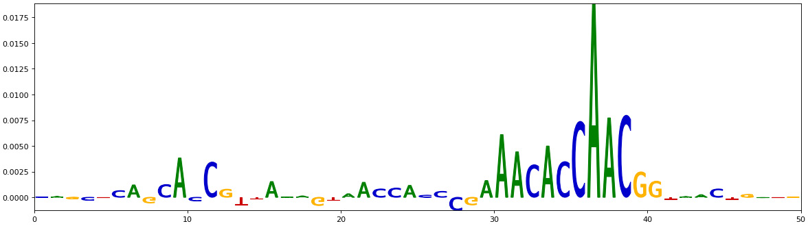
Figure 10.11 – Saliency map for bases of the positive sequences

The preceding saliency plot should show values for the AAACACCAACGG bases in the DNA sequence of one of the positive samples. Unfortunately, this is not exactly the motif that we inserted in the positive sequence. Our ground truth is AAAGAGGAAGTT This may have happened because we haven’t optimized the model enough or chosen the right model for training this data. This is where we can spend a lot of time doing optimization and model interpretation. Testing different hyperparameters is a good practice that may help to get a clear signal from this data.

Summary

Model interpretability is a relatively new area, with most publications happening in the last few years, but it is a very active area of research in DL now that is of utmost importance to realize the promise of precision medicine. The ability to interpret model decisions or predictions has several business advantages and can ultimately lead to higher profits. Because of model interpretability, more and more companies are leaning toward using DL models in their decision-making processes. This is not restricted to low-risk sectors but also high-risk sectors such as medicine and genomics too. If they are not currently using model interpretability, they plan to incorporate it into their future strategy.

This chapter is an attempt to introduce you to model interpretability, why it is important, why business organizations care about it, and different methods for performing model interpretability, specifically for black-box models such as DNNs in the genomics field. The chapter started with the basics of what is model interpretability, why we care, and what value model interpretability brings to the business. With the advances in the model interpretability method, currently, there are both model-agnostic and black-box-specific models proposed to explain black-box models and we have looked at several of them broadly classified into global and local methods. Each of the methods has its advantages and disadvantages. General guidance is provided to pick the right method for model interpretability. The key takeaway from those methods is that the features used by the black-box model can be interpreted, which is important for biological domains. Finally, we looked at how to interpret models using protein binding site predictions as an example When business organizations incorporate model interpretability into their DL life cycle, it’s an iterative cycle, and it results in higher profitability. For non-profits, NGOs, and research organizations, profits might not be a motive. Still, it is useful for them to keep the preceding things in mind to avoid inaccurate decision-making—reputation is at stake. Now that we have understood model deployment and hopefully improved the model, we are ready to deploy the model in production in the next chapter.